Characteristic Basis Function Method for Solving
Electromagnetic Scattering Problems Over Rough
Terrain Profiles
Atacan Yagbasan, Celal Alp Tunc, Member, IEEE, Vakur B. Ertürk, Member, IEEE,
Ayhan Altintas, Senior Member, IEEE, and Raj Mittra, Life Fellow, IEEE
Abstract—A computationally efficient algorithm, which com-bines the characteristic basis function method (CBFM), the physical optics (PO) approach (when applicable) with the forward backward method (FBM), is applied for the investigation of elec-tromagnetic scattering from—and propagation over—large-scale rough terrain problems. The algorithm utilizes high-level basis functions defined on macro-domains (blocks), called the charac-teristic basis functions (CBFs) that are constructed by aggregating low-level basis functions (i.e., conventional sub-domain basis func-tions). The FBM as well as the PO approach (when applicable) are used to construct the aforementioned CBFs. The conventional CBFM is slightly modified to handle large-terrain problems, and is further embellished by accelerating it, as well as reducing its storage requirements, via the use of an extrapolation procedure. Numerical results for the total fields, as well as for the path loss are presented and compared with either measured or previously published reference solutions to assess the efficiency and accuracy of the algorithm.
Index Terms—Characteristic basis functions (CBFs), method of moments (MoM), forward-backward method (FBM), electromag-netic scattering, terrain propagation.
I. INTRODUCTION
M
ANY military and commercial applications, such as mobile radio planning, require an accurate estimation of the scattered field or path loss for an arbitrary environ-ment. Consequently, accurate and efficient investigation of electromagnetic scattering from and propagation over largeManuscript received April 08, 2009; revised October 30, 2009; accepted November 19, 2009. First published March 01, 2010; current version published May 05, 2010. This work was supported by the Turkish Academy of Sciences (TÜBA)-GEB˙IP.
A. Yagbasan is with the Department of Electrical and Electronics Engi-neering, Bilkent University, Bilkent, Ankara TR-06800, Turkey and also with Aselsan Electronics Inc., Ankara TR-06800, Turkey.
C. A. Tunc is with the Department of Electrical and Electronics Engineering, Bilkent University, Ankara 06800, Turkey and also with the Ankara Research and Technology Laboratory (ARTLAB Ltd.), Ankara TR-06540, Turkey.
V. B. Ertürk is with the Department of Electrical and Electronics En-gineering, Bilkent University, Bilkent, Ankara TR-06800, Turkey (e-mail: [email protected]).
A. Altintas is with the Department of Electrical and Electronics Engineering, Bilkent University, Bilkent, Ankara TR-06800, Turkey and also with the Com-munications and Spectrum Management Research Center (ISYAM), Bilkent University, Bilkent, Ankara TR-06800, Turkey.
R. Mittra is with the Electromagnetic Communication Laboratory, The Penn-sylvania State University, University Park, PA 16802 USA.
Color versions of one or more of the figures in this paper are available online at http://ieeexplore.ieee.org.
Digital Object Identifier 10.1109/TAP.2010.2044334
scale rough terrain profiles [1], [2] is an important area of research in computational electromagnetics. Various integral equation (IE)-based methods, such as the well-known Method of Moments (MoM), have been used for perfectly [3]–[12] and imperfectly [13]–[18] conducting rough terrain profiles. The direct solution of a set of linear algebraic equations requires an operational count on the order of [i.e., ], where is the number of unknowns, and this is computationally very expensive for large problems. This prompts us to use iterative methods for electrically large rough surfaces [5]–[18], where the storage and computation cost requirements are reduced to per iteration. Among them, the stationary iterative forward-backward method (FBM), proposed in [8], is the most efficient one, and it yields an accurate solution to the problem with only a few iterations when the system of equations is not ill-conditioned. Also, it can be further accelerated by using the spectral acceleration (SA) algorithm [10] to reduce the operation count to and to decrease the memory require-ments as well. The spectrally accelerated forward-backward method (SA-FBM) has been successfully applied to large terrain problems modeled via the use of impedance boundary conditions (IBC) [14]–[18] and to layered rough surfaces [19] as well.
Recently, a new technique referred to as the characteristic basis function method (CBFM) has been proposed for the ef-ficient solution of the MoM matrix equation [20]. It is based on constructing high-level basis functions on macro-domains, that are referred to as the characteristic basis functions (CBFs), by aggregating conventional sub-domain basis functions, and their use leads to a reduced matrix equation that can be solved by di-rect solvers for many cases without the need to iterate. In this paper, the CBFM is combined with the physical optics (PO) ap-proach (when applicable) and the FBM (the method is hence referred to as CBFM-PO-FBM) for accurate and efficient so-lution of electromagnetic scattering and propagation problems over rough terrains. The present approach retains many prop-erties of the conventional CBFM [20], but embellishes it by using the PO (when applicable) as well as the FBM to gen-erate the CBFs. Briefly, the terrain is partitioned into blocks, each of which contains many sub-domain basis functions. Then, primary basis functions (PBFs) and secondary basis functions (SBFs), which comprise the CBFs, are obtained by using either the PO (when applicable) and/or the FBM. Finally, a new matrix equation is derived by using the abovementioned CBFs, leading to a significantly small-size matrix—referred to as the reduced
matrix—that can be solved directly by using the LU decompo-sition without using iteration and/or preconditioner. Note that the two important attributes of the conventional CBFM are: (i) It rigorously accounts for the mutual interaction effects through the use of SBFs. (ii) It is iteration-free. Note that recently di-rect solvers that can handle up to million unknowns have been introduced [21]. Furthermore, multilevel CBFM [22] can also be implemented for extremely large terrains, which makes the direct solution for the corresponding reduced matrix feasible. Thus, CBFM is a very attractive choice for analyzing electro-magnetic scattering problems involving large-scale and signifi-cantly rough terrain profiles [23].
In this work, we introduce certain modifications of the con-ventional CBFM to tailor it for terrain problems, with a view to improving both the computational cost as well as the memory storage requirements of the original method. First of all, because the mutual interactions between far away elements on a terrain are very weak, only the mutual interactions between the adja-cent blocks are retained in finding the SBFs. However, addi-tional blocks located further away can be included, if desired, if their contributions are significant. In addition, an extrapolation procedure is used during the generation of the reduced matrix. We note that further modifications of the proposed algorithm (i.e., CBFM-PO-FBM) are under progress to apply it to re-en-trant surfaces, where FBM fails and the generalized forward backward method (GFBM) [11] is generally used. We also note that CBFM has been used to compute the radar cross section (RCS) of two-dimensional (2-D) faceted objects [24], as well as of three-dimensional (3-D) bodies [25], with good results. Further improvements on CBFM (different from the extrapola-tion algorithm proposed in this paper) have also been proposed in [26]–[28] before.
In Section II, the integral equation formulation and its solution via CBFM-PO-FBM are briefly discussed. Certain modifications of the conventional CBFM to ensure its fast and accurate implementation for scattering problems involving large scale rough terrain profiles are also discussed in this section. Numerical results for the total fields and the associ-ated path loss characteristics are presented, and are compared with measured as well as the previously-published reference solutions in Section III to demonstrate the accuracy and the numerical efficiency of CBFM-PO-FBM. A brief discussion of some of the parametric tests that are performed on such terrains is also included. An time convention, where is the angular frequency, is employed and suppressed throughout this paper.
II. FORMULATION
Let us consider a one-dimensional (1-D) rough terrain geometry characterized by the surface height profile , de-fined by along the -axis, which is embedded in a 2-D space ( - plane), as illustrated in Fig. 1. Both the surface-height profile and the electromagnetic fields are as-sumed to be constant along the -direction. It is asas-sumed that the terrain is an imperfect conductor, modeled by the surface
impedance ) along the surface via the use
of the IBC [29].
Fig. 1. Problem Geometry.
For the transverse magnetic ( : with respect to -coordi-nate) polarization the electric field integral equation (EFIE) can be written as
(1) where is the incident electric field, is the equivalent surface current density (in the -direction). A magnetic field integral equation (MFIE) can be constructed in a similar fashion for the transverse electric polarization in terms of the tangential surface current density, . It reads;
(2) where is the incident magnetic field. In (1) and (2), ) is the 2-D free-space Green’s function; is the wave number in air; is the out-going unit normal vector to the surface at the radiating point ; and are the permittivity and permeability of free-space, re-spectively. Although the terrain extends from minus infinity to infinity in , the incident field is considered to be tapered so that the illuminated rough surface, and consequently, the integrations in (1) and (2) can be confined to a finite region of length . Furthermore, in the case where the terrain is illumi-nated by an antenna, it is placed near the edge of the terrain (i.e., ), such that the field at that edge (i.e., behind that antenna) is weak [19]. Then, the conventional MoM procedure involving the discretization of IEs given by (1) and (2), and application of point-matching with pulse basis functions, leads to a matrix equation
(3) where is the ( : number of surface unknowns) MoM impedance matrix whose entries are given in [15]; is the excitation vector such that its elements are the incident fields
evaluated at the matching points; and, is the solution vector that contains the unknown current coefficients.
The starting point of the CBFM-PO-FBM is the same as that of the conventional CBFM where the terrain profile is parti-tioned into distinct blocks, where is the number of
un-knowns in block (i.e., ). Let and be
the current and excitation vectors for the th block, respectively, and the matrix block containing the interactions between groups and is . The exact solution for given that is known, for , can be found by solving
(4)
where is the th diagonal (self) block. Next step is to construct a set of high-level basis functions, namely the CBFs, which represent each block (a portion of the terrain profile) by using (4) such that
(5) (6) First, the PBFs, , that take all self-interactions of block into account may be found directly from (5) because is known. However, to eliminate the spurious edge effects at the block truncations, each block is extended in both directions by
; hence, each extended block has unknowns .
As a result, PBFs are constructed for each extended block by solving the equation ([20])
(7) where is the self impedance matrix of the ex-tended block , and is the excitation vector cor-responding to this block, which is a subset of that includes the rows belonging to block . The concept of block matrices and the extended blocks are illustrated in [20]. Although these PBFs represent the self-interactions within the blocks, they will only serve as basis functions, which would be used to construct the reduced matrix. Thus, their accurate evaluation, particularly for large scale terrain geometries where each block may con-tain a significantly large number of unknowns, is not necessary at this stage. Consequently, (7) can be solved using an iterative technique as opposed to direct inversion such as the LU decom-position, as in [20]. Moreover, depending on the nature of the electromagnetic source that is used to illuminate the terrain pro-file, one can even use the PO to construct the PBFs, and thereby bypass the need to solve (7). In this study, PBFs are found by using either a single iteration of FBM, or the PO to accelerate the method. It has been observed that, one can safely use the PO if the terrain is illuminated by an isotropic radiator located at a few wavelengths above the terrain, or by a plane wave. However, if the terrain is illuminated by a directive antenna (for instance a dipole) located at a few wavelengths above the terrain, then using the PO yields inaccurate results for the induced current, which, in turn also affects the accuracy of the scattered field.
In any event, PBFs are generated at the end of this step by following the procedure described above. Our next step is to construct the SBFs, , from (6) that account the mu-tual interactions among the blocks. However, is not known a priori. Therefore, as an approximation, we use PBFs to rep-resent in (6), and using the extended blocks SBFs can be found by solving
(8) The justification for the abovementioned approximation is be-cause the form of is not expected to be strongly dependent on the exact form of . Besides, similar to PBFs, accurate evaluation of SBFs is not required at this stage. Hence, only a single iteration of FBM is used in (8) to achieve the compu-tational efficiency. Note that the right-hand side of (8) may be physically interpreted as the electric field impressed on block due to the current in block , and the matrix is formed from the original MoM matrix by selecting the testing loca-tion at the extended block , with the source localoca-tion being the block . Furthermore, special care is required for the evalua-tion of the right-hand side of (8), since it deals with an extended block. If the extended block (which contains the test locations) shares a number of unknowns with block (which contains the source locations), these source locations should be identified and eliminated from and . Thus, if we let be that
number, sizes of and become and
, respectively. On the other hand, if the extended block and block are far-away blocks (i.e., there is no overlap due to the extension of the blocks), then the sizes of and
become and , respectively.
In the conventional CBFM, the expansion given by (4) results
in CBFs ( PBFs and SBFs) as opposed to
sub-sectional basis functions. However, in 1-D electrically large ter-rain problems, mutual interactions among the far-away blocks are very weak, and we can take advantage of this fact to further reduce the number of unknowns. Therefore, in this study only the SBFs associated with mutual interactions between the adja-cent blocks are retained (i.e., for block , SBFs are constructed for blocks and ). Note that the two end-blocks have single SBFs. Consequently, the total number of SBF turns out to be , and we end up with a total of CBFs. At this point it should be mentioned that if more SBFs are included (i.e., more neighboring blocks are included on each side of the extended block ), the accuracy of the CBFM-PO-FBM solution (taking FBM as a reference solution) improves up to a certain degree and then saturates. However, such an accuracy improve-ment is not uniform throughout the terrain; it is more dominant close to the source region. Unfortunately, for extremely large terrains it brings significant computational burden and memory requirements during the construction of the reduced matrix, as explained below. Therefore, including more blocks than only the adjacent ones during the construction of the SBFs is not fol-lowed in this work (except for the case where a parametric test on the number of SBFs is performed).
After constructing all the CBFs, the solution to the entire problem is expressed as a linear combination of CBFs
(under the assumption that only the adjacent blocks are included during the construction of the SBFs) given by
..
. ...
..
. (9)
where is the unknown complex expansion coefficient for the th basis function of block . Substituting (9) into (3), the solution can be cast into the following form:
(10) where
(11) Note that in (11) is the MoM impedance matrix given in (3), generated by selecting the observation points in block and source points in block . It differs from used in (8) in the sense that is not an extended matrix since the extension parts are truncated prior to (9).
Also note that in (10), are now the large-support basis functions, and to generate the reduced matrix (and hence, to find ) large-support testing functions are required. Thus, using Galerkin method and selecting the testing functions as the Her-mitian of , the reduced matrix with a rank of is gen-erated. It should be mentioned that a different formulation for the generation of the reduced matrix is presented in [30], where the basis functions are the CBFs and the testing functions are the Hermitian of the CBFs that leads to the same reduced ma-trix generated in this paper.
The solution of the resultant matrix equation yields the un-known expansion coefficients, , for the CBFs. Accurate so-lution of the reduced matrix equation is critical at this step and, hence, direct solvers are preferred. In fact, the direct solution of this system poses little additional computational burden, since
is significantly smaller compared to .
Although only the adjacent blocks are used to find the SBFs, all blocks are involved during the generation of the reduced ma-trix. Therefore, the most time-consuming and main memory-in-tensive parts of the method are the storage of and the gen-eration of the reduced matrix. As illustrated in the numerical examples, the computational cost for the generation of is , whereas it is for the generation of the re-duced matrix (to take the inner product of both sides of (10) with the hermitian of ). Therefore, a simple extrapolation
procedure is used in the CBFM-PO-FBM algorithm to reduce the necessary computation time and the memory requirement for the generation of . Because the vectors actually rep-resent the entire domain fields of the induced current on the entire th block, it is observed that their amplitudes vary rela-tively slowly, and that their phase variation is almost linear over small regions formed from the discretization of the entire ter-rain. Hence, during the generation of vectors using (11), ratively small groups are assumed whose elements will be the el-ements of , denoted by . The number of elements in each group is basically governed by the roughness of regions (occu-pied by each group) along the terrain such that abrupt roughness variations are usually selected as the borders of these groups. In practice, these groups are composed of 10, 50 or 100 elements (in some cases more than 100 elements can be used). Then, as-suming a linearly varying phase and a constant amplitude for the ’s within each group, only two elements at the middle (i.e., and ) are calculated using (11), the phase difference between them is computed, and the values of the re-maining elements in the group are determined from
(12) which corresponds to a linear interpolation in phase and a con-stant amplitude assumption. In (12), is the constant ampli-tude, is the phase difference between the two elements located in the middle (i.e., the phase difference between and ), and is the number of elements in the group. As a result, for a group of elements ( may vary from group to group), a factor of is defined to indicate the amount of acceleration in the computation time and the savings from the memory requirements during the generation of . Although this procedure requires a modest amount of pre-processing, it is relatively easy to implement, and it can accelerate the gen-eration of by a factor of (effective acceleration factor), which is given by
(13)
where is the factor of the th group, is the total number of groups, is the length of the th group and is the length of the entire terrain. Experience shows that typically ranges between 10 and 20 for the real-world terrain profiles considered in this paper.
III. NUMERICALRESULTS
The CBFM-PO-FBM algorithm, together with the aforemen-tioned extrapolation procedure, has been tested to solve total fields and/or path loss for the various terrain profiles. The results are compared with the measured data, as well as with the previ-ously-published reference solutions. In all examples considered in this paper, a point-matching technique that uses rectangular pulse-shaped basis functions with pulse width has been utilized. The -axis of all plots represents the horizontal dis-tance, and the source is located at .
The first set of the results pertain to the comparison of the CBFM-PO-FBM results with the measurements and the
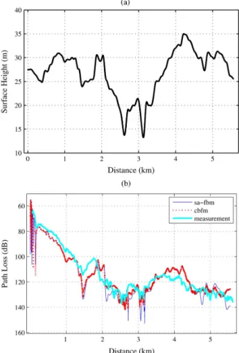
Fig. 2. Path Loss over Hadsund terrain profile. Distance 7931 m, N = 115000. (a) Hadsund Terrain Profile, (b) TM Polarization at 435 MHz.
SA-FBM. The selected terrains, namely Hadsund and Jerslev terrain profiles illustrated in Figs. 2(a) and 3(a), respectively, are from Denmark. The measured data is obtained from [31], derived by using a transmitting dipole located at a height of 10.4 meters with a transmitted power of 10 Watts and a gain of 8 dBi. The receiving antenna is a monopole, located on top of a van at a height of 2.4 meters. More information regarding the transmitting and receiving antennas can be found
in [31]. A surface impedance value is used
in order to handle some small vegetations and other types of land covers along the profiles. The path loss results for TM polarization at 435 MHz over Hadsund and at 970 MHz for Jerslev profiles are presented in Figs. 2(b) and 3(b), respec-tively. To generate the CBFM-PO-FBM results, the Hadsund terrain, that is 7931 meters long, is expanded using 115 000 basis functions at 435 MHz. Then, it is divided into 100 blocks (i.e., ) and 298 CBFs (in the form of 100 PBFs and 198 SBFs) are used. The corresponding values for the 5446
meters long Jerslev profile are; at 970 MHz,
and the total number of CBFs is 298 (in the form of 100 PBFs and 198 SBFs), respectively. It has been observed that the selection of smaller values up to does not change the accuracy of the path-loss results significantly. However, a choice of yields less accurate path-loss results. In the generation of CBFs, PBFs and SBFs are obtained via a single iteration of FBM. For both terrains, blocks are
Fig. 3. Path Loss over Jerslev terrain profile. Distance 5446 m,N = 180000. (a) Jerslev Terrain Profile, (b) TM Polarization at 970 MHz.
extended by approximately (i.e., ) to suppress the spurious edge effects. Extensions less than yields small accuracy problems for the current, but such problems are not visible in the path-loss. Extensions beyond showed little improvement in the accuracy. A non-uniform extrapolation procedure, detailed in the previous section, is implemented to accelerate the generation of the vectors. The number is selected to be large at relatively flat portions of the terrains, which correspond to 0–2 km range for the Hadsund terrain and 0.75–1.5 km for the Jerslev terrain, and is used for the rest. As a result, the generation of is accel-erated by approximately 12.5 and 11 times, for the Hadsund and Jerslev profiles, respectively. As seen in Figs. 2(b) and 3(b), CBFM-PO-FBM results are in good agreement with both measurements and SA-FBM that verifies the accuracy of the method. Finally, the required CPU time for CBFM-PO-FBM is 8105 seconds for the Hadsund and 15972 seconds for the Jerslev profiles, whereas it is 125 seconds per iteration, and an overall 10 iterations (hence, 1250 seconds) for the Hadsund and 164 seconds per iteration, and again 10 iterations (hence, 1640 seconds) for the Jerslev profiles when SA-FBM is used. Note that SA-FBM, being an type method, is much faster than CBFM-PO-FBM. However, SA-FBM is also expected to exhibit some problems for very rough surfaces, in particular when there are large height variations along the terrain.
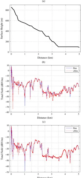
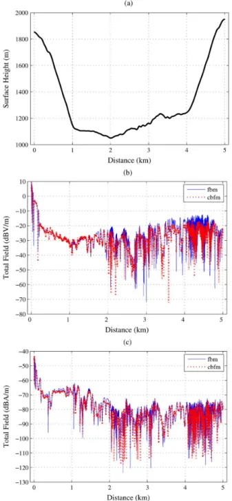
Fig. 4. Total Field (TM Polarization) over a terrain profile from the west side of Turkey, Distance 5000 m,N = 50000. (a) Terrain Profile, (b) 50 Blocks, (c) 200 Blocks.
Fig. 4(a) illustrates a 5 kilometer portion of a downhill terrain profile taken from the west side of Turkey that has a height vari-ation of approximately 700 meters. The terrain is illuminated by an isotropic radiator with 25 Watts output at 300 MHz located at 25 meters above . The receiver height is 2.4 meters. The total field results for both TM and TE polarizations are obtained via CBFM-PO-FBM and compared with the FBM. Total field
results for and are given in Fig. 4(b), (c)
for TM polarization, and Fig. 5(b), (c) for TE polarization. In all cases, PBFs are obtained by using the PO, and the blocks are extended by to suppress the edge effects. We note that the agreement between the FBM and the CBFM-PO-FBM results
Fig. 5. Total Field (TE Polarization) over a terrain profile from the west side of Turkey, Distance 5000 m,N = 50000. (a) Terrain Profile, (b) 50 Blocks, (c) 200 Blocks.
is good in all cases presented. However, we go on to perform several parametric tests for this terrain to test the robustness of CBFM-PO-FBM, and to see if it handles the problem efficiently for other terrain profiles. Towards this end, we use the following criterion for the residual error:
(14)
where indicates the Frobenius norm, and and
are the FBM and CBFM-PO-FBM results, respectively. Note that we have used the FBM result as the
TABLE I
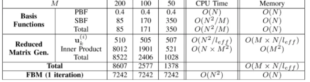
COMPARISON OFCPU TIMES OFCBFM-PO-FBM WITHFBM,AND THEERROR FOR THETERRAINPROFILE INFIG. 4(A)FORVARIOUSM VALUES, N = 50000; l = 15
TABLE II
CPU TIMES FORDIFFERENTSTAGES OFCBFM-PO-FBMFOR THETERRAINPROFILEDEPICTED INFIG. 4(A), TM POLARIZATION,N = 50000;l = 15
reference solution. We observe that the accuracy of the method increases with increasing , as seen from the last column in Table I. Moreover, the improvement in the accuracy is notice-able when we compare Figs. 4(b) and 5(b) with Figs. 4(c) and 5(c), respectively. However, such an increase in the accuracy comes at the expense of increased CPU time as shown in the ‘Total CPU (s)’ column of Table I, because we need to calculate additional inner products during the generation of the reduced matrix. However, we point out that even the most expensive case (i.e., ) the CPU time for the CBFM-PO-FBM is comparable to that needed for a single iteration in the FBM, for either the TM or the TE polarizations, and that 6 and 2 iterations are required to generate accurate FBM results for the TM and TE polarizations, respectively. We note further, that the required CPU time needed in the implementation of the CBFM-PO-FBM is approximately 5 times less than that of a single iteration FBM for the TM case when .
Details about the CPU times and the storage requirements for different stages of CBFM-PO-FBM for this example are presented in Table II. It is evident that an increase in in-creases the time needed to generate the reduced matrix. More specifically, the share of the inner product operations of the CBFM procedure begins to dominate the CPU times, since its computational cost is . It is note-worthy, however that, the use of the extrapolation procedure reduces the required CPU time for the generation of the vectors from to . Note also that further increase of does not bring an important reduction in terms of CPU times. It is also obvious that the CPU time needed to generate the CBFs are rel-atively negligible when compared to the total time. In this ex-ample since PO is used for the generation of PBFs, this step does not depend on , and requires very little time [recall that the operational count for PO is ]. However, since we use FBM while generating the SBFs, the required CPU times for the generation of SBFs and the number of blocks, , are inversely proportional to each other. Hence, with a major decrease in , the generation of the SBFs can become a dominant part of the CBFM procedure. Finally for this example, the time required to
TABLE III
COMPARISON OFCPU TIMES OFCBFM-PO-FBMWITHFBMANDERRORS FOR THETERRAINPROFILE INFIG. 4(A)FORVARIOUSnnbVALUES, TM
POLARIZATION,l = 15; N = 50000
invert the reduced matrix is negligible, since the matrix size is quite small.
Next, we perform another parametric test on this terrain in which we increase the number of neighboring blocks, denoted by , gradually so that more SBFs are included. As an ex-ample means 4 neighboring blocks are included (i.e.,
for the extended block and
are included). Using the same error criterion as given by (14), Table III presents the CPU times and the errors for var-ious values. In all cases, the number of PBFs is 50 (since
).
As seen in Tables III and IV, the CPU time increases signif-icantly for an increase in the SBFs due to the additional inner products that need to be calculated during the generation of the reduced matrix. In common with Table II, Table IV shows the details of the CPU times and storage requirements associated with the different stages of CBFM-PO-FBM for various values. Note that the generation of SBFs, vectors and the performance of the inner products are the stages that are directly affected by the number of values.
It should be noted that for all practical purposes, we only need to implement the CBFM-PO-FBM algorithm by taking only the adjacent blocks (i.e., ) for the generation of SBFs.
In all cases, we employ a non-uniform extrapolation for this terrain as follows: Up to approximately 3 kilometers is used uniformly. Beyond 3 kilometers the value of is increased to 50, since the terrain profile is flatter. As a result, is com-puted 15 times faster (i.e., ). However, as a final test,
TABLE IV
CPU TIMES FORDIFFERENTSTAGES OFCBFM-PO-FBM WITHVARIOUSnnb VALUES FOR THETERRAINPROFILEDEPICTED INFIG. 4(A), TMPOLARIZATION, N = 50000;M = 50; l = 15
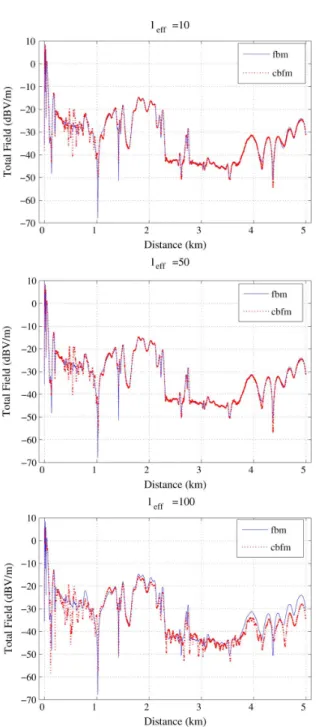
Fig. 6. Total Field (TM Polarization) for variousl = l values for the terrain profile depicted in Fig. 4(a) whenM = 200 and nnb = 2.
is varied uniformly (hence, ) to see when the used ex-trapolation scheme begins to yield inaccurate results.
TABLE V
CPU TIMES ANDERROR OFCBFM-PO-FBMFORVARIOUSl VALUES WHENnnb = 2FOR THETERRAINPROBLEM INFIG. 4(A) (TM POL.). FOR
CBFM,M = 200; N = 250AND THENUMBER OFCBFS IS598
Fig. 6 shows the comparison of CBFM-PO-FBM results with
those of FBM for various values ( and 100
cases) when and . As seen from the figure
as well as from the last column of Table V, the error increases as increases, as expected, although the CPU time decreases, also as expected.
For the last example, we employ the same set of parameters as well as the same procedure (i.e., same transmitter and re-ceiver locations and properties, same frequency, same polariza-tions, same approach to the construction of CBFs) for a 5 kilo-meter portion of a valley-like terrain profile, shown in Fig. 7(a). The terrain represents the east-side of Turkey and has a height variation of approximately 800 meters. Parametric tests similar to those performed in the previous numerical examples are re-peated and the results are presented in Tables VI and VII.
The value of is chosen for the construction of the SBFs in all of the examples in this set. Comparisons of the total field results obtained via CBFM-PO-FBM and FBM are shown in Fig. 7(b) and (c) for the TM and TE polarizations, respec-tively, when . In common, with previous cases, good agreement is obtained yet again for this profile. As expected, a larger value of is used for the middle parts of the ter-rain and the value is decreased to 10 for the rougher sections that are located at the two ends of the terrain. As a result, an acceleration of is obtained during the process of gen-erating the vectors .
Before closing, we provide a brief summary of the storage requirements of the CBFM-PO-FBM algorithm as well as of the parametric tests that we have performed about its robustness, efficiency and accuracy.
• Storage Requirements of CBFM-PO-FBM: We have already discussed how the CPU times vary as we change certain parameters such as and . Likewise, the memory requirement of the CBFM-PO-FBM al-gorithm also changes with the above parameters as shown in Tables II and IV. One of the advantages of the CBFM-PO-FBM is that it does not require the storage of a
Fig. 7. Total Field over a terrain profile from the east side of Turkey, Distance 5000 m,N = 50000; M = 200 and nnb = 2. (a) Terrain Profile, (b) TM Polarization, (c) TE Polarization.
TABLE VI
COMPARISON OFCPU TIMES OFCBFM-PO-FBMANDFBMFOR THETERRAIN PROFILE INFIG. 7(A)FORVARIOUSM VALUES,N = 50000;l = 19
matrix, except for the reduced matrix, provided that we do not use direct solvers for the generation of basis functions, which is the case for this study. Since basis functions
TABLE VII
CPU TIMES FORDIFFERENTSTAGES OFCBFM-PO-FBMFOR THETERRAIN PROFILEDEPICTED INFIG. 7(A), TM POLARIZATION,N = 50000;l = 19
are generated via the use of PO (when applicable) and/or FBM, the impedance matrices are not stored. However, we do need to store the basis functions as well as the vec-tors for the generation of the reduced matrix. The memory requirement for the basis functions can be estimated to be
, and it is for the
vectors. Thus, the total memory requirement is given by (15) for . When we include additional mutual
interac-tions (i.e., ), the factor is replaced by
the corresponding values given in Table III. Evidently, the dominating part of the above sum is the storage of vec-tors which is for large values. Fortunately, with the use of the extrapolation procedure, significant re-duction can be obtained for the memory storage.
• Extension of Blocks: During the generation of PBFs (re-gardless of the method used) and SBFs, the blocks are ex-tended by approximately . Extensions less than yield small inaccuracies in the results for the induced current, although these inaccuracies do not affect the scattered or total field results (and hence, path-loss results). Extensions beyond do not noticeably improve the results, either for the induced currents or for the scattered fields.
• Number of Blocks: The choice of number of blocks, , is flexible. However, some issues such as efficiency and accuracy should be considered prior to start simulations. From the efficiency point of view when increases, the generation of the reduced matrix (due to the inner prod-ucts) dominates the operational count , whereas when small values of are chosen, then the generation of the CBFs (due to one iteration of FBM)
dominates the operational count. On the other hand, an in-crease in , improves the accuracy of both the conven-tional CBFM and the CBFM-PO-FBM algorithm proposed in this paper (at the expense of increased CPU time and storage requirements as mentioned above). It has been ob-served that an increase in improves the accuracy pri-marily in the regions far away from the source. In all ex-amples considered in this paper (and in many others not reported in this paper) either an isotropic or a dipole type source is located at location of the terrain, and signif-icant improvement in the scattered/total fields is observed at regions far away from the source. In the regions close to the source, the accuracy of the results improves as well,
but since the field amplitudes are higher in those regions, such improvements are not all that noticeable. Note that in the limiting case when equals to (total number of unknowns) and all the blocks are included, the CBFM (as expected) reverts to the conventional MoM.
Considering the abovementioned efficiency and accuracy issues, we usually start out terrain simulations by selecting . Based on the storage and operational count requirements, which are known for each stage of the CBFM-PO-FBM algorithm, an initial adjustment on the value of can be done. However, small variations in values do not have a significant impact both on the accuracy and the efficiency of the method.
• Number of Neighboring Blocks (i.e., Number of SBFs): In common with the situation where the number of blocks are increased, an increase in the number of neighboring blocks to be included in the generation of the SBFs im-proves the accuracy of both the conventional CBFM as well as that of the CBFM-PO-FBM algorithm proposed in this paper, but only up to a certain level and, of course, at the expense of increased CPU time and storage require-ments. Since in an electrically large terrain, mutual teractions among the far-away blocks are very weak, in-cluding additional neighboring blocks does not improve the overall accuracy significantly, and in a uniform fashion. However, when the field points are close to the source re-gion (isotropic or dipole type antennas at ), we observe a significant improvement if the two neighboring blocks (rather than only the adjacent blocks) on each side of the extended block are included. This is an expected result because, field values of the blocks that are close to the excitation are stronger, and taking an additional neigh-boring block into account from this region improves the accuracy especially around this region. However, the in-crease of the CPU time, as well as of the storage require-ments again becomes an issue in this case.
IV. CONCLUSION
An iteration-free and efficient algorithm, which combines the conventional CBFM, the PO (when applicable), and/or the FBM, has been employed in this work to solve the problem of scattering from —and propagation over— large-scale and rough terrain problems. The resultant method, referred to as the CBFM-PO-FBM, is basically a modified version of the conventional CBFM such that it is tailored for the analysis of large, rough terrain profiles. The CBFM-PO-FBM is further accelerated, and its storage requirement is reduced by using a non-uniform extrapolation procedure based on the linear phase approximation. The developed algorithm has been applied to many 1-D rough terrain geometries that have significant height variations, and it has not suffered from any converge problems as long as the profiles are not re-entrant. Accuracy and efficiency of the method have also been tested from these applications by comparing the results with that of available methods or measurements. As a result, the CBFM-PO-FBM can be safely used in the investigation of large-scale, rough terrain geometries that may have very large height deviations. Research on further acceleration of the algorithm, as well as its
extension of the technique to re-entrant surfaces, is currently under study.
ACKNOWLEDGMENT
The authors thank Dr. R. J. Burkholder (ElectroScience Lab., The Ohio-State University) for his valuable comments on the presentation of CBFM, and Prof. J. B. Andersen (Aalborg Uni-versity, Denmark) and his associates for kindly providing the terrain profiles as well as the results obtained by the integral equation method [31].
REFERENCES
[1] L. Tsang, J. A. Kong, and K.-H. Ding, Scattering of Electromagnetic
Waves: Theories and Applications. New York: Wiley, 2000. [2] L. Tsang, J. A. Kong, K.-H. Ding, and C. O. Ao, Scattering of
Electro-magnetic Waves: Numerical Simulations. New York: Wiley, 2001. [3] R. Axline and A. Fung, “Numerical computation of scattering from a
perfectly conducting random surface,” IEEE Trans. Antennas Propag., vol. 26, no. 3, pp. 482–488, May 1978.
[4] D. Colak, R. J. Burkholder, and E. H. Newman, “Multiple sweep method of moments analysis of electromagnetic scattering from 3D targets on ocean-like rough surfaces,” Microw. Opt. Technol. Lett., vol. 49, no. 1, pp. 241–247, 2007.
[5] C. Smith, A. Peterson, and R. Mittra, “The biconjugate gradient method for electromagnetic scattering,” IEEE Trans. Antennas Propag., vol. 38, no. 6, pp. 938–940, Jun. 1990.
[6] F. Chen, “The numerical calculation of two-dimensional rough surface scattering by the conjugate gradient method,” Int. J. Remote Sensing, vol. 17, no. 4, pp. 801–808, 1996.
[7] D. A. Kapp and G. S. Brown, “A new numerical method for rough-surface scattering calculations,” IEEE Trans. Antennas Propag., vol. 44, no. 5, pp. 711–721, May 1996.
[8] D. Holliday, L. L. DeRaad, and G. J. St-Cyr, “Forward-backward: A new method for computing low-grazing angle scattering,” IEEE Trans.
Antennas Propag., vol. 44, no. 5, pp. 722–729, May 1996.
[9] P. Tran, “Calculation of the scattering of electromagnetic waves from a two-dimensional perfectly conducting surface using the method of or-dered multiple interaction,” Waves Random Media, vol. 7, pp. 295–302, 1997.
[10] H.-T. Chou and J. T. Johnson, “A novel acceleration for the compu-tation of scattering from rough surfaces with the forward-backward method,” Radio Sci., vol. 33, no. 5, pp. 1277–1287, Jun. 1998. [11] M. R. Pino, L. Landesa, J. Rodriguez, F. Obelleiro, and R. Burkholder,
“The generalized forward-backward method for analyzing the scat-tering from targets on ocean-like rough surfaces,” IEEE Trans.
An-tennas Propag., vol. 47, no. 6, pp. 961–969, Jun. 1999.
[12] J. West and J. Sturm, “On iterative approaches for electromagnetic rough-surface scattering problems,” IEEE Trans. Antennas Propag., vol. 47, no. 8, pp. 1281–1288, Aug. 1999.
[13] J. West, “Integral equation formulation for iterative calculation of scattering from lossy rough surfaces,” IEEE Trans. Geosci. Remote
Sensing, vol. 38, no. 4, pp. 1609–1615, Jul. 2000.
[14] H.-T. Chou and J. Johnson, “Formulation of forward-backward method using novel spectral acceleration for the modeling of scattering from impedance rough surfaces,” IEEE Trans. Geosci. Remote Sensing, vol. 38, no. 1, pp. 605–607, Jan. 2000.
[15] J. A. López, M. R. Pino, F. Obelleiro, and J. L. Rodríguez, “Applica-tion of the spectral accelera“Applica-tion forward-backward method to coverage analysis over terrain profiles,” J. Electromagn. Waves Applicat., vol. 15, pp. 1049–1074, Aug. 2001.
[16] D. Torrungrueng and J. T. Johnson, “The forward-backward method with a novel spectral acceleration algorithm (FB/NSA) for the com-putation of scattering from two-dimensional large-scale impedance random rough surfaces,” Microw. Opt. Technol. Lett., vol. 29, no. 4, pp. 232–236, 2001.
[17] B. Babaoglu, A. Altintas, and V. B. Erturk, “Spectrally accelerated bi-conjugate gradient stabilized method for scattering from and propaga-tion over electrically large inhomogeneous geometries,” Microw. Opt.
Technol. Lett., vol. 46, no. 2, pp. 158–162, 2005.
[18] C. A. Tunc, A. Altintas, and V. B. Ertürk, “Examination of existent propagation models over large inhomogeneous terrain profiles using fast integral equation solution,” IEEE Trans. Antennas Propag., vol. 53, no. 9, pp. 3080–3083, Sep. 2005.
[19] C. Moss, T. Grzegorczyk, H. Han, and J. Kong, “Forward-back-ward method with spectral acceleration for scattering from layered rough surfaces,” IEEE Trans. Antennas Propag., vol. 54, no. 3, pp. 1006–1016, Mar. 2006.
[20] V. V. S. Prakash and R. Mittra, “Characteristic basis function method: A new technique for efficient solution of method of moments matrix equa-tions,” Microw. Opt. Technol. Lett., vol. 36, no. 2, pp. 95–100, 2003. [21] J. Shaeffer, “Direct solve of electrically large integral equations for
problem sizes to 1 m unknowns,” IEEE Trans. Antennas Propag., vol. 56, no. 8, pp. 2306–2313, Aug. 2008.
[22] C. Delgado, E. Garcia, F. Catedra, and R. Mittra, “Hierarchical scheme for the application of the characteristic basis function method based on a multilevel approach,” presented at the IEEE Antennas and Propaga-tion Society Int. Symp., San Diego, CA, Jul. 5–11, 2008.
[23] A. Yagbasan, C. A. Tunc, V. B. Erturk, A. Altintas, and R. Mittra, “Ap-plication of characteristic basis function method for scattering from and propagation over terrain problems,” presented at the Int. URSI Commission B-Electromagnetics Theory Symp., Ottawa, Canada, Jul. 26–28, 2007.
[24] G. Tiberi, S. Rosace, A. Monorchio, G. Manara, and R. Mittra, “Elec-tromagnetic scattering from large faceted conducting bodies by using analytically derived characteristic basis functions,” IEEE Antennas
Wireless Propag. Lett., vol. 2, pp. 290–293, 2003.
[25] R. Mittra, J.-F. Ma, E. Lucente, and A. Monorchio, “CBMOM -an it-eration free MoM approach for solving large multiscale EM radiation and scattering problems,” in Proc. IEEE Antennas and Propagation
So-ciety Int. Symp., Jul. 2005, vol. 2B, pp. 2–5.
[26] G. Tiberi, A. Monorchio, G. Manara, and R. Mittra, “A spectral do-main integral equation method utilizing analytically derived character-istic basis functions for the scattering from large faceted objects,” IEEE
Trans. Antennas Propag., vol. 54, no. 9, pp. 2508–2514, Sep. 2006.
[27] E. Lucente, A. Monorchio, and R. Mittra, “Generation of characteristic basis functions by using sparse MoM impedance matrix to construct the solution of large scattering and radiation problems,” in Proc. IEEE
Antennas and Propagation Society Int. Symp., 2006, pp. 4091–4094.
[28] E. Lucente, A. Monorchio, and R. Mittra, “An iteration-free MoM approach based on excitation independent characteristic basis func-tions for solving large multiscale electromagnetic scattering problems,”
IEEE Trans. Antennas Propag., vol. 56, no. 4, pp. 999–1007, Apr. 2008.
[29] T. B. A. Senior, “Impedance boundary conditions for imperfectly con-ducting surfaces,” Appl. Sci. Res., vol. 8, pp. 418–436, 1961. [30] S. J. Kwon, K. Du, and R. Mittra, “Characteristic basis function method:
A numerically efficient technique for analyzing microwave and rf cir-cuits,” Microw. Opt. Technol. Lett., vol. 38, no. 6, pp. 444–448, 2003. [31] J. Hviid, J. Andersen, J. Toftgard, and J. Bojer, “Terrain-based
propaga-tion model for rural area-an integral equapropaga-tion approach,” IEEE Trans.
Antennas Propag., vol. 43, no. 1, pp. 41–46, Jan. 1995.
Atacan Yagbasan received the B.S. and M.S. degrees from Bilkent University, Ankara, Turkey, in 2006 and 2009, respectively.
He is currently a Ph.D. student in the Middle East Technical University (METU), Ankara. Also, he has been working for Aselsan Electronics Incorporated, Ankara, as an RF and Microwave Design Engineer since 2006. His research interests include numerical techniques for electromagnetic scattering from rough surface profiles.
Celal Alp Tunc (S’01–M’09) received the B.Sc. de-gree in electronics and communication engineering from Istanbul Technical University, Istanbul, in 2001 and the M.Sc. and Ph.D. degrees in electrical and electronics engineering from Bilkent University, Ankara, in 2003 and 2009, respectively.
Between 2001 and 2009, he worked as a teaching and research assistant at Bilkent University, Elec-trical and Electronics Engineering Department. Afterwards, he served in the Turkish Armed Forces as a tank team commander with the rank of second lieutenant. He is currently pursuing research and development activities at Ankara Research and Technology Laboratory (ARTLAB Ltd.) of which he is a co-founder. His research areas are numerical techniques for computational
electromagnetics, large scale electromagnetic radiation-scattering problems, antenna analysis and propagation channel modeling for MIMO wireless communications, design and production of microstrip MIMO antenna arrays, MIMO channel measurements, optimization techniques and algorithms for electromagnetic/information theoretic problems.
Dr. Tunc is a recipient of the Young Scientist Award of URSI in 2008.
Vakur B. Ertüurk (M’00) received the B.S. degree in electrical engineering from the Middle East Technical University, Ankara, Turkey, in 1993, and the M.S. and Ph.D. degrees from The Ohio-State University (OSU), Columbus, in 1996 and 2000, respectively.
He is currently an Associate Professor with the Electrical and Electronics Engineering Department, Bilkent University, Ankara. His research interests include the analysis and design of planar and con-formal arrays, active integrated antennas, scattering from and propagation over large terrain profiles and metamaterials.
Dr. Ertürk served as the Secretary/Treasurer of the IEEE Turkey Section as well as the Turkey Chapter of the IEEE Antennas and Propagation, Microwave Theory and Techniques, Electron Devices and Electromagnetic Compatibility Societies. He was the recipient of the 2005 URSI Young Scientist and 2007 Turkish Academy of Sciences Distinguished Young Scientist Awards.
Ayhan Altintas (SM’93) received the B.S. and M.S. degrees from Middle East Technical University, Ankara, Turkey and the Ph.D. degree from Ohio State University, in 1979, 1981, and 1986, respec-tively, all in electrical engineering.
Currently, he is Professor and Chair of Electrical Engineering at Bilkent University, Ankara, Turkey. He is also the Director of Communication and Spec-trum Management Research Center (ISYAM).
Dr. Altintas was the Chairman of IEEE Turkey Section for the terms 1991–1993 and 1995–1997. He is the founder and first chair of the IEEE AP/MTT Chapter in the Turkey Section. At present, he is the National Chair of URSI Commission B (Scat-tering and Diffraction). His research interests are in electromagnetics, antennas, propagation, and wireless communication systems. He is a Fulbright Scholar, and an Alexander von Humboldt Fellow. He received the Ohio State University ElectroScience Laboratory Outstanding Dissertation Award of 1986, IEEE 1991 Outstanding Student Branch Counselor Award, 1991 Research Award of Prof. Mustafa N. Parlar foundation of METU, and Young Scientist Award of Scientific and Technical Research Council of Turkey (Tubitak) in 1996. He is a member of Sigma Xi and Phi Kappa Phi and a recipient of IEEE Third Millennium Medal.
Raj Mittra (S’54–M’57–SM’69–F’71–LF’96) is a Professor in the Electrical Engineering Department, Pennsylvania State University, where he is also the Director of the Electromagnetic Communication Laboratory, which is affiliated with the Commu-nication and Space Sciences Laboratory of the EE Department. Prior to joining Penn State he was a Professor in the Electrical and Computer Engi-neering Department, University of Illinois in Urbana Champaign. He has about 1000 publications to his credit that include 31 books or book chapters on electromagnetics, antennas, microwaves and electronic packaging.
Prof. Mittra is a Life Fellow of the IEEE, a Past-President of AP-S, and he has served as the Editor of the IEEE TRANSACTIONS ONANTENNAS AND PROPAGATION. He has been awarded the Guggenheim Fellowship, the IEEE Centennial and Millennium Medals, the IEEE/AP-S Distinguished Achieve-ment Award, the AP-S Chen-To Tai Distinguished Educator Award, and the Electromagnetics Award of the IEEE. He has supervised the completion of 100 Ph.D. theses, an equal number of M.S. theses, and has mentored over 50 post-docs. He is the President of RM Associates, which is a consulting organization that provides services to industrial and governmental organizations, both in the U. S. and abroad.