Activity analysis for assistive systems

ACTIVITY ANALYSIS FOR ASSISTIVE SYSTEMS

A THESIS

SUBMITTED TO THE DEPARTMENT OF COMPUTER ENGINEERING AND THE GRADUATE SCHOOL OF ENGINEERING AND SCIENCE

OF BILKENT UNIVERSITY

IN PARTIAL FULFILLMENT OF THE REQUIREMENTS FOR THE DEGREE OF

MASTER OF SCIENCE

By

Ahmet ˙Is¸cen

August, 2014

I certify that I have read this thesis and that in my opinion it is fully adequate, in scope and in quality, as a thesis for the degree of Master of Science.

Assist. Dr. Pınar Duygulu S¸ahin(Advisor)

I certify that I have read this thesis and that in my opinion it is fully adequate, in scope and in quality, as a thesis for the degree of Master of Science.

Assist. Prof. Dr. ¨Oznur Tas¸tan

I certify that I have read this thesis and that in my opinion it is fully adequate, in scope and in quality, as a thesis for the degree of Master of Science.

Assist. Prof. Dr. Sinan Kalkan

ABSTRACT

ACTIVITY ANALYSIS FOR ASSISTIVE SYSTEMS

Ahmet ˙Is¸cen

M.S. in Computer Engineering Supervisor: Assist. Dr. Pınar Duygulu S¸ahin

August, 2014

Although understanding and analyzing human actions is a popular research topic in computer vision, most of the research has focused on recognizing ”ordinary” actions, such as walking and jumping. Extending these methods for more specific domains, such as assistive technologies, is not a trivial task. In most cases, these applications contain more fine-grained activities with low inter-class variance and high intra-class variance.

In this thesis, we propose to use motion information from snippets, or small video intervals, in order to recognize actions from daily activities. Proposed method encodes the motion by considering the motion statistics, such as the variance and the length of trajectories. It also encodes the position information by using a spatial grid. We show that such approach is especially helpful for the domain of medical device usage, which contains actions with fast movements

Another contribution that we propose is to model the sequential information of actions by the order in which they occur. This is especially useful for fine-grained activities, such as cooking activities, where the visual information may not be enough to distinguish between different actions. As for the visual perspective of the problem, we propose to combine multiple visual descriptors by weighing their confidence val-ues. Our experiments show that, temporal sequence model and the fusion of multiple descriptors significantly improve the performance when used together.

¨

OZET

YARDIMCI TEKNOLOJ˙I S˙ISTEMLER˙INDE AKT˙IV˙ITE

ANAL˙IZ˙I

Ahmet ˙Is¸cen

Bilgisayar M¨uhendisli˘gi, Y¨uksek Lisans Tez Y¨oneticisi: Yrd. Doc¸. Pınar Duygulu S¸ahin

A˘gustos, 2014

˙Insan hareketlerini anlamak ve analiz etmek bilgisayarlı g¨or¨u alanında ne kadar pop¨uler bir konu olsa da, yapılan aras¸tırmaların c¸o˘gu y¨ur¨umek ve zıplamak gibi ola˘gan hareketleri tanımak ¨uzerine yo˘gunlas¸maktadır. Bu y¨ontemleri yardımcı teknolojiler gibi daha spesifik alanlarda uygulamak her zaman kolay olmayabilir. Bu uygulamalar c¸o˘gu zaman sınıflar arası c¸ok az de˘gis¸im g¨osteren ve aynı sınıf ic¸inde fazla de˘gis¸im g¨osterebilen aktivitelerden olus¸maktadır.

Bu tezde videoların k¨uc¸¨uk parc¸alarından hareket bilgisini kullanarak g¨unl¨uk ak-tiviteleri tanımayı ¨oneriyoruz. ¨Onerilen y¨ontem, g¨osterilen hareketi tanımlamak ic¸in hareket y¨or¨ungesinin varyans ve uzunluk gibi istatistiksel bilgilerini kullanmaktadır. Aynı zamanda, hareketlerin konumsal bilgileri de uzaysal grid kullanılarak elde edilir. Deneylerimizde bu y¨ontemin ¨ozellikle ic¸inde hızlı hareketler bulunduran tıbbi cihaz kullanımı alanında yardımcı oldu˘gunu g¨or¨uyoruz.

Bu tezdeki di˘ger katkı ise, g¨orsel bilginin yeterli olmadı˘gı zamanlarda hareket-lerin sıralamasını modellemenin sistemin aktivite tanıma performansı arttırdı˘gı g¨ostermektir. Problemin g¨orsel kısmı ic¸inse, farklı ¨oznitelik gruplarının tahminlerini birles¸tiren bir ¨oneriyle, birden fazla g¨orsel bilgi kullanabiliyoruz. Deneylerimizde gos-terdi˘gi ¨uzere, ¨onerilen y¨ontemler tıbbi cihaz kullanımı ve yemek yapma aktivitelerini tanıma gibi yardımcı teknoloji cihazları alanlarında performansı ciddi bir s¸ekilde yukseltmis¸tir.

Acknowledgement

Firstly, I would like to thank Assist. Prof. Dr. Pınar Duygulu S¸ahin for giving me a chance to work with her, introducing me to the field of computer vision, and supporting and guiding me throughout my degree. I would like to thank the members of my thesis committee, Assist. Prof. Dr. ¨Oznur Tas¸tan and Assist. Prof. Dr. Sinan Kalkan for accepting to review my thesis.

I was privileged to collaborate with great people during my Master’s degree through internships at Yahoo Research Barcelona and Inria Rennes. I would like to thank Dr. Barla Cambazoglu and Dr. Ioannis Arapakis from Yahoo Research Barcelona, and Dr. Herv´e J´egou, Dr. Giorgos Tolias, and Dr. Philippe-Henri Gos-selin from Inria Rennes for guiding me during my stay at their institutions. I would also like to thank my adviser, Dr. Pınar Duygulu S¸ahin for allowing me to visit those institutions during my degree.

I want to thank the members of Bilkent RETINA research group and the other grad-uate students of the Computer Engineering Department, for their assistance, kindness and more importantly friendship. I also would like to thank all the professors who guided and motivated us, and all the staff who made it possible for us to work in the best conditions possible. I also would like to thank my suite-mates from 15th Dormi-tory who I enjoyed being neighbors with for a year and a half. It is not easy for most people to like Ankara, but I would like to give my sincere thanks to the great friends of mine from Middle Eastern Technical University, who I knew before coming to Ankara, and made it possible for me to really enjoy this city with amazing memories.

Finally, I would like to deeply thank my parents and my beautiful sisters, for their never-ending support, motivation, and love. I am proud to have such a beautiful family, and I was able to come this far in life thanks to the values and virtues you have taught and the education you have provided.

This thesis is partially supported by TUBITAK project with grant no 112E174 and CHIST-ERA MUCKE project.

Contents

1 Introduction 1

2 Background and Related Work 5

2.1 Dense Trajectory Sampling in Videos . . . 5

2.1.1 Dense Sampling . . . 5

2.1.2 Trajectories . . . 7

2.1.3 Trajectory Descriptors . . . 8

2.2 Related Work . . . 10

3 Describing Human Actions for Assistive Technologies 12 3.1 Snippet Trajectory Histograms . . . 13

3.1.1 Finding Trajectories . . . 13

3.1.2 Calculating Snippet Histograms . . . 14

CONTENTS vii

3.2.2 Inhaler Usage . . . 18

3.2.3 Infusion Pump Usage . . . 22

3.2.4 Cooking Activities . . . 26

4 Recognizing Tiny and Fine-Grained Activities 29 4.1 Visual Model With Multiple Feature Descriptors . . . 31

4.1.1 Training Individual Classifiers for Each Feature Space . . . . 33

4.1.2 Finding a Confidence Factor For Each Classifier . . . 34

4.1.3 Combining Individual Classifiers . . . 35

4.2 Temporal Coherence Model of Activities . . . 35

4.3 Making a Final Decision . . . 37

4.4 Experiments . . . 38

4.4.1 Cooking Activities . . . 38

4.4.2 Infusion Pump Usage . . . 43

List of Figures

1.1 Our task is to detect activities for cooking activities [1] and medical de-vice usage, more specifically for infusion pump [2] and inhaler dede-vices [3] . An example of infusion pump usage is shown on the first row, and inhaler usage is shown on the second row. There are recordings from 3 different camera angles for infusion pump usage. . . 3

2.1 Visualization of trajectories. Figure taken from [4]. . . 5

2.2 Visualization of dense trajectories process.Figure taken from [4]. . . . 6

2.3 Densely sampled points to extract trajectories. Points from homoge-neous regions are removed. Figure taken from [4]. . . 7

2.4 Visualization of descriptors. Figure taken from [4]. . . 8

3.1 Visualization of Snippet Histograms technique. A small interval of a video is taken, and the motion information is aggregated. A histogram based on the length and the variance statistics of this motion, as well as its spatial location, is created . . . 15

LIST OF FIGURES ix

3.3 The effect of overlap rate threshold. Based on this figure, we choose t “ 0.5 as the overlap rate in our experiments. . . 20

3.4 Example of the shaking action from the Inhaler Dataset [3]. Regardless of the position which the user shakes the inhaler device, we get many long trajectories placed on the left or the right of the screen. . . 21

3.5 Example of position checking action from the Inhaler Dataset [3]. Po-sition checking is more subtle action than shaking. The user may slowly or suddenly move the device towards his or her face. As a result, we get trajectories of varying lengths for this action. . . 22

3.6 Example of extracted trajectories for the same frame from the Infusion Pump Dataset [2]. We can more motion information from the cameras positioned above and side, compared to the camera positioned in front of the user . . . 23

3.7 Frames of the subject performing very similar actions.The subject is performing cut apart on the top row, cut dice on the second row, cut sliceson the third row, and cut-off ends on the last row. . . 25

3.8 Frames of the subject performing very similar actions.The subject is performing cut apart on the top row, cut dice on the second row, cut sliceson the third row, and cut-off ends on the last row. . . 28

4.1 An example of high intra-class variance from the cooking activities dataset [1]. Same action may be performed differently by different subjects. . . 30

4.2 An example of low inter-class variance from the cooking activities dataset [1]. Different actions may look similar visually. . . 30

LIST OF FIGURES x

4.3 In our classification framework, we classify a newly observed activ-ity x by considering its preceding activities and spatio-temporal visual descriptors. For the example above, we consider only 2 previous ac-tivities which are cut slices and cut dice. Our model classifies x as put

in bowl, which is an accurate decision. . . 31

4.4 The framework for visual model explained in Section 4.1 . . . 32

4.5 Temporal sequence example. . . 36

4.6 The framework for temporal model explained in Section 4.2 . . . 36

4.7 Classification by using visual information only. Our combination method surpasses feature concatenation (abbreviated as ”CONCTD.” on the chart) in all subjects except for 18. . . 39

4.8 An example where neither visual classifiers nor temporal sequence model can make the correct decision. The subject performs two dif-ferent actions on the right column, namely spice on the top, and pour on the bottom. These two actions look visually similar, and has the same preceding action open cap. Therefore, our system fails for such cases. . . 42

List of Tables

3.1 Comparison of Snippet Histograms with other trajectory based de-scriptors for the shaking action of Inhaler Dataset. Trajectory scores are the same as those reported in [3] . . . 19

3.2 Comparison of position checking action results. Although RGB-based descriptors are nowhere close to the depth video performance in [3], Snippet Histograms still perform better than other trajectory-based de-scriptors . . . 21

3.3 Results for Pump Dataset. The performance for each camera is re-ported separately, and the best performance among three cameras is reported under the fusion column. . . 24

3.4 Comparison of Snippet Histograms with other trajectory based de-scriptors for the cooking dataset. . . 27

4.1 Classification by using only the temporal coherence information. . . 39

4.2 Visual Information + Controlled Temporal Coherence . . . 40

4.3 Visual Information + Semi-Controlled Temporal Coherence . . . 40

LIST OF TABLES xii

4.5 Comparison of temporal sequence model used with different descrip-tors. We also compare our results with the ROI-BoW method intro-duced in [2]. For this experiment, we only report the best result ob-tained among 3 cameras for each method . . . 43

Chapter 1

Introduction

Understanding, predicting, and analyzing human actions can be a challenging task not only for computers, but also for humans. With the advancement of technology and internet, research in human activity recognition has improved dramatically over the recent years. The early research was focused on basic activities that are easily distin-guishable, such as human body movements like walking, bending, punching etc. More recently, a significant amount of the research is focused on recognizing ordinary ac-tions from movies [5] or sports [6]. Most of these methods can be extended to introduce solutions that may have a more direct impact in our lives. Some of these applications can include video surveillance, anomaly detection, and daily activity analysis.

In addition to recognizing ordinary actions, the need for recognition of more spe-cific activities that can be similar to each other, or fine-grained human activities, has also gained big demand due to new possible applications. One such application is the elderly care. As the elderly population has been increasing, monitoring individual’s homes has become an important issue to reduce the cost of care. Due to increasing costs, more and more patients decide to use such devices at home to save money and time. However, with the lack of experience and failure to follow instructions, personal usage of such devices may be ineffective, or even worse, they may cause fatal prob-lems. In fact, U.S. Food and Drug Administration reported 56,000 incidents between 2005 and 2009, including deaths and injuries, caused by incorrect infusion pump us-age [7]. With the impracticality of supervising every patient for using medical devices

correctly, there is a clear need for assistive systems that detect incorrect device usage, and report it to the patient.

Another example of a fine-grained activity classification problem is the classifica-tion of cooking activities. Some of the activities, such as cut apart, cut off ends and cut slicesare shown on Figure 1.1. These activities look very similar to each other, and it is often difficult to decide which feature descriptor to use in order to obtain the best classification result. Furthermore, some feature descriptors can work well in some subset of activities, while others give better results in other subset of activities.

This thesis focuses on two assistive system applications; cooking activities and medical device usage; more specifically infusion pump and inhaler device usage. Cooking activities can be viewed as fine-grained activities; specific activities with very low inter-class variability. These activities, such as cut slices, cut stripes, cut in, are not very different from each other, and are hard to classify only using the visual in-formation. Therefore, solving this problem remains an important challenge in activity recognition domain. Infusion pumps are used to deliver fluid and medication into a patient’s body, and inhaler devices are used for asthma therapy. The main challenge is to recognize a subject’s daily activities accurately, and these activities are usually very similar to each other with low inter-class variance. Another challenge is that, some actions, called tiny actions may consist of only a very little movement by certain parts of the body.

On the contrary, as such methods are developed for a specific purpose, we can make some assumptions when developing a new method. As an example, we can as-sume that the camera will usually record the user from a certain perspective, therefore certain actions may happen in specific positions. In fact, Cai et al. make use of this information to detect actions for infusion pump usage [2]. Another assumption we can make is that there most likely will not be a camera motion when the patient performs an action, as the camera is always expected to stay put when the usage takes place.

Figure 1.1: Our task is to detect activities for cooking activities [1] and medical device usage, more specifically for infusion pump [2] and inhaler devices [3] . An example of infusion pump usage is shown on the first row, and inhaler usage is shown on the second row. There are recordings from 3 different camera angles for infusion pump usage.

listed above. Moreover, because of their simplicity, it is possible to implement and use Snippet Histograms in real time applications. We show that the proposed Snippet Histogram method performs very well for our tasks, outperforming other trajectory-based descriptors.

When considering daily activities to be recognized by an assistive living system, we can argue that there is an order in activities. As an example, we can argue that when someone enters a kitchen, they follow a certain sequence of activities when they are cooking. In that sequence, certain activities are more likely to come after the others. For example, when someone performs the activity cut dice, just by considering a normal cooking process, our intuition tells us that the subject might want to put whatever they have cut into a bowl, and the next activity is likely to be put in bowl.

Our second contribution makes use of this property to help recognize actions. We develop a model to capture temporal sequence model of activities, in order to predict which activities would occur based on what has happened before. Note that this model does not use any visual information originally, but only keeps track of the order of activities. We show that when combined with the visual information, it improves the recognition performance significantly.

The rest of this thesis is organized as follows. Chapter 2 gives background informa-tion on densely extracting trajectories from videos, and reviews the related work in the literature. Chapter 3 introduces the Snippet Histograms and explains how to construct them. We also introduce the datasets we use, and show our experimental results in those datasets using Snippet Histograms. Chapter 4 introduces the temporal sequence model of activities, as well as combining multiple descriptors for classification pur-poses. We also report experimental results using these models. Chapter 5 concludes this thesis.

Chapter 2

Background and Related Work

2.1

Dense Trajectory Sampling in Videos

In this section, we summarize the work of Wang et al.[4] on dense trajectories, which is the foundation of the work we will introduce in this thesis. We will refer to their method as dense trajectories from now on. This method samples and tracks dense trajectories from video frames using the optical flow information, and extracts visual descriptors from these densely sampled trajectories. It is considered to be the state-of-art for many action recognition tasks.

2.1.1

Dense Sampling

The first step of the algorithm is to sample initial dense points on a spatial grid. These points are sampled similar to dense features used in image domain. They are sampled

Figure 2.2: Visualization of dense trajectories process.Figure taken from [4].

using a step size of W pixels on each spatial scale separately. The authors found that using W “ 5 and 8 spatial scales results in optimal performance, where the scaling factor between each spatial scale is 1{?2.

After sampling initial points, we need to remove the ones that correspond to ho-mogeneous areas. Hoho-mogeneous areas are areas without any textural structure, such as the sky, and it is shown for many applications that these regions do not provide any helpful information for feature descriptors. Moreover, since the purpose of this method is to track these points for a number of frames, these points need to be removed since it would be impossible to track them.

In order to remove the homogeneous points, authors propose to use the eigenvalues of the auto-correlation matrix, such that the points on the grid are removed if their eigenvalues are less than a threshold T :

T “ 0.001 ˆ max iPI minpλ 1 i, λ 2 iq (2.1)

Figure 2.3: Densely sampled points to extract trajectories. Points from homogeneous regions are removed. Figure taken from [4].

2.1.2

Trajectories

After sampling dense points on the spatial grid, the algorithm finds trajectories by calculating the optical flow field ωt “ put, vtq, where ut and vt are the horizontal

and vertical components of the optical flow respectively. This flow field is calculated between each point Pt “ pxt, ytq on frame It and its following frame It`1. In order

to eliminate the noise, the authors apply median filter on ωt, so that the point Pt`1is

estimated as:

Pt`1“ pxt`1, yt`1q “ pxt, ytq ` pM ˚ ωtq|xt,yt (2.2)

where M is the median filtering kernel of size 3 ˆ 3 pixels. Each trajectory is formed by concatenating points of consequent frames pPt, Pt`1, Pt`2, . . . q. Because

trajectories are likely to move from their initial locations after the starting frame, the authors track them for L frames, where L “ 15. If no tracked point is found at the W ˆ W neighborhood during the tracking process, that trajectory is eliminated and a new point is sampled. Also, static trajectories and erroneous trajectories with very large displacements are removed.

Figure 2.4: Visualization of descriptors. Figure taken from [4].

2.1.3

Trajectory Descriptors

After trajectories are tracked, they are described using 4 different feature descriptors. In the following subsections, we explain these descriptors and the information they represent using the trajectories.

2.1.3.1 Trajectory Shape Descriptor

This is a simple descriptor encoding the shape of a trajectory, which is the displacement of each point from one frame to another, such that ∆Pt “ pPt`1 ´ Ptq “ pxt`1 ´

xt, yt`1´ ytq. We normalize the displacement values to obtain the final vector:

S “ ∆Pt “ pPt`1´ P<sub>řt`L´1</sub>tq “ pxt`1´ xt, yt`1´ ytq

j“t ||∆Pj||

(2.3)

The size of this descriptor depends on the trajectory size L, since it consists of displacement of x and y coordinates between each frame. As an example, for L “ 15, we obtain a 30-dimensional vector.

2.1.3.2 Histograms of Oriented Gradients and Histograms of Oriented Flow

Histograms of oriented gradients (HOG) and histograms of optical flows (HOF) [9, 5], are shown to be very useful descriptors for video [10]. These descriptors require space-time volumes aligned with trajectories in order to describe the visual information. The authors use a spatio-temporal grid of size nσ ˆ nσˆ nτ in a volume of N ˆ N pixels

and L frames, where N “ 32, nσ “ 2, nτ “ 3, and L is the trajectory length which is

set to 15 in the previous steps.

HOG and HOF encode different kind of visual information from motion. Orig-inally used as an image descriptor, HOG encodes the static appearance information, whereas HOF encodes the local motion information. For both descriptors, orientations are quantized into 8 bins and magnitudes are used for weighting. An additional 9th zero bin is added to HOF, in order to account for pixels whose optical flow magni-tudes are smaller than the threshold. As a result, HOG descriptor has 96 dimensions (2 ˆ 2 ˆ 3 ˆ 8) and HOF descriptor has 108 dimensions (2 ˆ 2 ˆ 3 ˆ 9).

2.1.3.3 Motion Boundary Histograms

MBH, or motion boundary histograms [11], provide a robust optical flow estimation which computes derivatives for horizontal and vertical components of optical flow sep-arately. By following such method, this descriptor eliminates the noise caused by cam-era motion, which may include tilting, zooming etc.

As mentioned, MBH separates optical flow field ωt “ put, vtq in horizontal and

ver-tical components, and calculates spatial derivative for each component. Then, similar to the HOG descriptor, orientation information is quantized into a histogram of 8 bins, weighted by their magnitude. This results in a 96 dimensional descriptor (2 ˆ2ˆ3ˆ8) for each horizontal and vertical components, called MBHx and MBHy, which are con-catenated to form the final feature vector MBH.

2.2

Related Work

Activity recognition is a widely studied topic in computer vision. The reader can refer to [12] for extensive survey on past human activity research. Some of the research, such as [13] focused on using interest points in order to recognize activities. Wang et al.[14] have shown that the human activity recognition can be improved by extracting densely sampled points from the frames. Although these activities rely on continuous video streams in order to recognize human activity, Ikizler et al. [15] have shown that it is possible to recognize human activity by only looking at still images. In the following, we give a brief overview of some of the early research in assistive living systems and temporal sequence modeling.

Even though most of the work focuses on finding “ordinary” actions [12], apply-ing them to the medical device usage or other assistive livapply-ing applications may not always be straight-forward. For example, dense trajectories method by Wang et al.[4] explained in Section 2.1 works very well for recognizing complex activities, however in this work we show that the simpler Snippet Histogram method outperforms it for the medical device usage applications.

Some of the research for activity recognition focus on applications involving daily activities. One of these applications is anomaly detection, which can be used for surveillance or assistive technologies. Roshtkari et al.[16] detects anomalous behav-iors by utilising a hierarchical codebook of dense spatio-temporal video volumes. Un-usual events are formulated as a sparse coding problem in [17]. Another interesting direction about unusuality detection is learning the crowd behavior [18], and then de-tecting anomaly as outliers [19]. Ziebart et al.predict people’s future locations [20] and Kitani et al.[21] forecasts human actions by considering the physical environment. Other works involving daily activities include daily action classification or summariza-tion by egocentric videos [22, 23, 24], fall detecsummariza-tion [25], and classificasummariza-tion of cooking actions [26, 27, 1, 28].

living technologies [33]. Fleck and Strasser [34] use cheap smartphone cameras for assisted living monitoring system. Smartphones are also used for obstacle detection for visually impaired people [35, 36]. There also applications that help visually impaired people with their grocery shopping [37], and that sonify images for them [38].

One of our main contributions in this thesis is similar to [2], who also analyze the use of infusion pump and inhaler devices. However, unlike their work we develop a method only using RGB videos, and not the depth information. Also, unlike [2] we aim for a real-time application which would be able to detect actions rapidly and warn the user if needed.

Modeling human action using sequential approaches to solve the human activity recognition problem has been examined in many works in the literature. These ap-proaches have modeled activity sequences using probabilistic models such as Hidden Markov Models or stochastic context-free grammars. One example is [39], where Iki-zler and Forsyth model human activities by HMMs. Other works such as [40, 41] have also used sequential and visual information for human activity recognition. One clear distinction of our work presented in this thesis from previous sequential approaches is that we do not model frames as sequences, but rather we model sequence of activities where each activity is a collection of frames.

Some classification methods for combination of different feature spaces have been proposed in [42]. More recently, Hashimoto et al.[43] have shown that it can be applied to current problems that require multiple feature spaces, but they ignore setting the reliability termand weigh each classifier the same.

For cooking related activities, there exist more than one databases that can be used. In addition to Rohrbach et al’s [1] MPII Cooking Activities Dataset, which will be explained in more detail in Section 3.2.4.1, TUM Kitchen Dataset [26] and CMU-Multimodal Activity Database [44] contain subjects performing kitchen activities, such as cooking, food preparation, or setting a table.

Chapter 3

Describing Human Actions for

Assistive Technologies

Although there have been many advancements in the recent years, human activity recognition remains to be a popular and unsolved problem in computer vision. Most of the work in the field involves finding “ordinary” actions, such as walking, running , or actions from movies or sports [5, 6]. Please refer to Section 2.2 for a more detailed review of the topic.

Applying existing human activity recognition methods to more specific applica-tions such as assistive living systems is not a trivial task, and may introduce additional challenges. First of all, each person may perform the same action in a different way. This causes high intra-class variance for action classes. Secondly, there may be more “tiny” actions, that have have very little movement, or “sudden” actions with rapid movement. Finally, for a useful daily application, proposed system must avoid expen-sive calculations and be able to work in real-time, and predict and recognize actions on the fly.

of their simplicity, it is possible to implement and use them in real time applications. Note that the proposed method only needs RGB videos, and not the depth information which is regularly used for such applications. We believe that, although the depth in-formation of a video is extremely useful for detecting some actions, an ordinary patient may not always have an access to a device with such capability. Therefore, we propose to investigate a method which would only use RGB video, and no depth information at all.

The rest of the chapter is organized as follows: Section 3.1 introduces the Snippet Trajectory Histograms. Experimental evaluation is provided in Section 3.2.

3.1

Snippet Trajectory Histograms

Originally introduced to detect unusual actions in videos [8], the Snippet Histograms method encodes the position and motion information in small intervals. It is built on dense sampling technique introduced by Wang et al.[4], which is used to produce the original motion trajectories from the video.

3.1.1

Finding Trajectories

Initial trajectories are found using the dense trajectory sampling method by Wang et al. [4]. This method samples feature points densely in different spatial scales with a step size of M pixels, where M “ 8 in our experiments. Sampled points in regions without any structure are removed since it is impossible to track them. Once the dense points are found, optical flow of the video is computed by applying the Farneb¨ack’s method [45]. Median filtering is applied to optical flow field to maintain sharp motion boundaries. Trajectories are tracked upto D frames apart, to limit drift from the original locations. Static trajectories with no motion information or erroneous trajectories with sudden large displacements are removed. Finally, a trajectory with duration D frames is represented as a sequence T “ pPt, ..., Pt`D´1q where Pt “ pxt, ytq is the point

trade-off between capturing fast motion, and providing sufficiently long trajectories with useful information [46].

3.1.2

Calculating Snippet Histograms

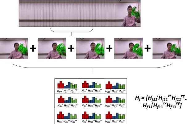
Unlike the trajectory feature [4], which encodes the shape of each trajectory, Snippet Histograms encode the motion information only by considering their statistical infor-mation. That is, for each trajectory T , we only use its length (l), variance along x-axis (vx), and variance along y-axis (vy). Length information is used in order to distinguish

between activities containing fast and small motions. Since trajectories are tracked for a fixed number of frames, longer trajectories correspond to faster motions, whereas smaller trajectories correspond to motions without much movement. Additionally, in order to encode the direction and the spatial extension of the motion, variance statistics in x and y coordinates are also used.

In order to aggregate motion statistics along with position, Snippet Histograms al-gorithm finds the average position of each trajectory during D frames which it was tracked for. First, for each trajectory T , we find its average position in x and y coor-dinates, mx and my respectively, along with its motion statistics. This can be done as

follows: mx “ 1 D t`D´1 ÿ t xt, vx “ 1 D t`D´1 ÿ t pxt´ mxq2 my “ 1 D t`D´1 ÿ t yt, vy “ 1 D t`D´1 ÿ t pyt´ myq2, l “ t`D´1 ÿ t a pxt`1´ xtq2` pyt`1´ ytq2 (3.1)

Hf11lHf11vxHf11vy

H

= [H

H

H

…

H

H

H

]

Figure 3.1: Visualization of Snippet Histograms technique. A small interval of a video is taken, and the motion information is aggregated. A histogram based on the length and the variance statistics of this motion, as well as its spatial location, is created

mx and my for each trajectory. We assign each trajectory to one of the spatial grids

based on their mx and my positions, and for each spatial grid, we create 3 histograms

by separately quantizing the l , vxand vyvalues of all the trajectories belonging to that

grid into b bins.

For example, let Hlptq be the frame histogram of length (l) values of all the

trajec-tories which are tracked until frame t. We create this histogram by concatenating b-bin histograms from each spatial bin, such that:

Hlptq “ pHlptqr1,1s, . . . Hlptqr1,N s, . . . HlptqrN,N sq (3.2)

where Hlptqri,js, 0 ď i, j ď N contains the b-bin histogram obtained by trajectories

whose average position lies in the ri, jsth_{cell. The same procedure is repeated for the}

vx and vyvalues of trajectories.

Now that we have the motion statistics of trajectories, they need to be aggregated in order to describe the overall motion in a small interval of the video. This is done by describing all the motion and position statistics in each small interval, which is also referred as snippets.

Snippet histograms are calculated for each frame in the video, and they encode the motion before and after the corresponding frame. As an example, for a given snippet size of S all the trajectories that end at frame f are summed, such that:

H_fl “ f `p}S}<sub>{</sub>2q ÿ t“f ´p}S}<sub>{</sub>2q Hlptq , Hfvx“ f `p}S}_{2q ÿ t“f ´p}S}_{2q Hvxptq H_fvy “ f `p}S}{2q ÿ t“f ´p}S}{2q Hvyptqq (3.3)

Hf “ rHfl, H vx f , H

vy

f s (3.4)

3.1.3

Snippet Histograms and Assistive Living Technologies

Our goal is to detect actions for assistive living technologies. We propose to use the Snippet Histograms method for a few properties of this domain, which we believe would be handled by Snippet Histograms.

First of all, we know that the camera will be standing still and looking over the user from a certain angle during the usage. Therefore, certain actions will always occur in certain spatial positions of the frame, since the position of each user will more or less be the same. Because Snippet Histograms divides the spatial coordinate into grids, and creates a separate histogram for each grid, we believe that it will help us to distinguish between similar actions taking place in different positions with respect to the user. The same idea is also applied in well know Spatial Pyramids method for images [47].

Secondly, some domains of assistive living technologies, like medical device usage, may involve very fast actions, such as shaking and very slow actions, such as opening a cap. By exploiting the statistical information of trajectories, such as the length and the variance of the trajectory motion, Snippet Histograms would enable us to separate fast actions from slow actions.

Lastly, due to their simplicity and easiness of the implementation, Snippet His-tograms would be suitable for real-time applications. In fact, the major overhead of computation is to generate initial trajectories using the dense trajectory method [4], but this can be sped up easily by downsampling the sizes of frames. In fact, in our ex-periments we found that downsampling the frames by a factor of 8 does not decrease the performance significantly. Once we have the initial trajectories, Snippet Histogram calculation requires only a few fast calculations.

3.2

Experiments

In this section, we explain our experiments using Snippet Histograms. First we give details about the implementation details of the methods, then for each task, we describe the dataset and report and discuss our results.

3.2.1

Implementation Details

For our implementation of Snippet Histograms to be used in our experiments, we ex-tracted initial snippets for D “ 15 frames. Then, we find Snippet Histograms in N ˆN spatial grid where N “ 3, and quantize length and variance information into b “ 5 bins. Therefore, we have 5 ˆ 3 ˆ 3 ˆ 3 “ 135 dimensional descriptors in the end. The size of each snippet is S “ 10 frames.

3.2.2

Inhaler Usage

3.2.2.1 Dataset

Inhaler Dataset [3] has 77 RGB and depth video recordings of users using Glaxo-SmithKline Inhalation Aerosol device. The user performs inhaler usage operation while sitting 50-70 cm in front of the camera. The dataset has 4 different action classes, shaking, where the user shakes the inhaler device, position checking, where the user puts the device about 2 inches in front of his or her mouth, inhaling and exhaling. However, since inhaling and exhaling actions cannot be detected visually, and need additional features such as audio, we do not evaluate them. We use recall, precision, and F-score measures for the evaluation of performance in this dataset.

(a) shaking (b) position checking (c) inhaling

Figure 3.2: Some of the actions in the Inhaler Dataset [3]. Although shaking and position-checking actions can be detected visually, inhaling and exhaling actions do not have any visual cues and require other modalities such as audio. Therefore, we do not include these two actions in our experiments.

Table 3.1: Comparison of Snippet Histograms with other trajectory based descriptors for the shaking action of Inhaler Dataset. Trajectory scores are the same as those reported in [3]

Trajectory HOG HOF MBH Snippet Hist Recall 95.31 50.00 100.00 87.50 98.44 Precision 91.04 22.70 91.43 71.79 100.00

F-score 93.13 31.22 95.52 78.87 99.21

3.2.2.2 Results

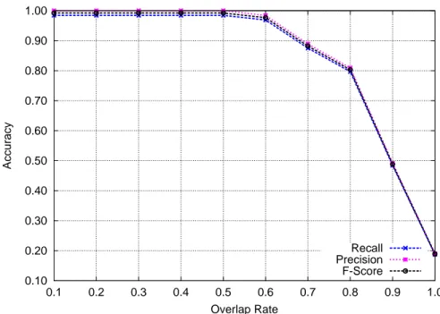
Our first set of experiments for this dataset with the Snippet Histograms is for the shaking action. Before we make any comparisons, we need to decide what we consider as a correct detection. We introduce the overlap ratio threshold t, which is the ratio of overlap in terms of frames between the detected action and the ground truth. If the detection and the ground truth frames has a greater overlap than t, then we consider it as a match.

As we see in Figure 3.3, the performance remains the same until t “ 0.5. This is also a reasonable threshold value for evaluation. Therefore, we set the overlap ratio threshold t “ 0.5, and conduct experiments to compare Snippets Histograms with other trajectory based descriptors.

0.10 0.20 0.30 0.40 0.50 0.60 0.70 0.80 0.90 1.00 0.1 0.2 0.3 0.4 0.5 0.6 0.7 0.8 0.9 1.0 Accuracy Overlap Rate Recall Precision F-Score

Figure 3.3: The effect of overlap rate threshold. Based on this figure, we choose t “ 0.5 as the overlap rate in our experiments.

from [4], with Snippet Histogram descriptors. Trajectory shape, HOG, HOF and MBH features are quantized into a BoW histogram with a codebook size of k “ 100.

Snippet histograms method has the highest overall F-score, having a perfect 100% precision score. The second-best performing descriptor is HOF, which is not a sur-prise, because it mostly encodes the flow information as well and not the appearance information. If we analyze the shaking action, such as the examples shown in Figure 3.4, we see that the it produces fast and long trajectories. Therefore, it is expected that these descriptors perform very well for this task.

Our second set of experiments is done for position checking. Note that we have no ways of checking the correct distance between the inhaler and the mouth only by using the RGB camera, however we just try to see if we can detect this action by the user’s motion.

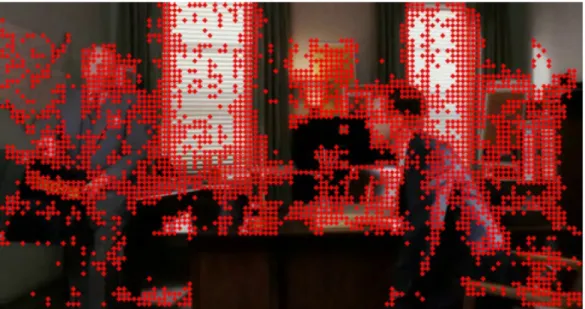
Figure 3.4: Example of the shaking action from the Inhaler Dataset [3]. Regardless of the position which the user shakes the inhaler device, we get many long trajectories placed on the left or the right of the screen.

Table 3.2: Comparison of position checking action results. Although RGB-based de-scriptors are nowhere close to the depth video performance in [3], Snippet Histograms still perform better than other trajectory-based descriptors

Trajectory HOG HOF MBH Snippet Hist Depth Recall 8.82 8.82 13.24 10.29 30.88 90.30 Precision 17.07 12.77 16.36 24.24 18.46 78.80 F-score 11.63 10.43 14.63 14.45 23.11 84.20

Histograms still have the best F-score when compared with the other trajectory-based descriptors, though it is really low.

One of the reasons for such a low score for trajectory-based features in this task is that the motion of moving the inhaler device towards the mouth differs dramatically from user to user. Some users move it suddenly, resulting in long trajectories, whereas others move it very subtly, as shown in Figure 3.5. Therefore, we must make use of depth, face and other information for this task, as done in [3], to obtain a reasonable performance.

3.2.2.3 Discussion

Based on our experiments, we show that the Snippet Histograms are very effective es-pecially for the shaking action detection for inhaler device usage. Because this action consists of sudden and fast movements, Snippet Histograms can encode the movement

Figure 3.5: Example of position checking action from the Inhaler Dataset [3]. Position checking is more subtle action than shaking. The user may slowly or suddenly move the device towards his or her face. As a result, we get trajectories of varying lengths for this action.

statistics in a way which clearly distinguishes them from other actions. When com-pared with other trajectory-based features, we see that it outperforms other descriptors except for the recall metric, where HOF obtains the top score. This is also somewhat expected, as HOF uses the pure flow information of optical flow field, which would capture this kind of movement. Also as expected, HOG has the worst performance among different detectors. This is because the shaking action does not require any ap-pearance information to be recognized, and only using apap-pearance information is not enough to distinguish from other actions.

For the position checking action, our experiments show that it is much more effec-tive to recognize it using a depth camera. In fact, the nature of the activity requires a depth camera to be used, as we would need to check the distance between the device and the user to warn if they are holding the device too close or too far. Using only RGB information with trajectory-based features is not suitable for this task.

3.2.3

Infusion Pump Usage

(a) front (b) side (c) above

Figure 3.6: Example of extracted trajectories for the same frame from the Infusion Pump Dataset [2]. We can more motion information from the cameras positioned above and side, compared to the camera positioned in front of the user

port, cap tube end/arm port, clean tube end/arm port, flush using syringe, and con-nect/disconnect. There are three different cameras recording each user synchronously from the side, above and front of the user. The dataset has both RGB and depth videos of these recordings, however we only make use of the RGB videos in this paper.

3.2.3.2 Results

As before, we compare the performance of Snippet Histograms with other trajectory-based features such as trajectory shape, HOG, HOF and MBH. These features are quantized into a BoW histogram with a codebook size of k “ 100.

In order to show the effect of each camera, we report scores separately for each camera in Table 3.3, as well as taking the best result among 3 cameras and reporting it under the fusion column. One of the points that we can observe from these results is that the camera from above seems to work better for trajectory-based features than the others. This can be explained by the fact that there is more movement when looked from above compared to side or front during the infusion pump usage (see Figure 3.6). Since these descriptors depend on trajectories of motion, they work better when there is more motion on camera. Compared to other descriptors, Snippet Histograms slightly have better performance in this task.

Table 3.3: Results for Pump Dataset. The performance for each camera is reported separately, and the best performance among three cameras is reported under the fusion column.

Actions Trajectory HOG

front side above fusion front side above fusion Turn the pump on/off 65.40 65.40 67.30 67.30 67.13 58.82 72.32 72.32

Press buttons 56.23 63.32 71.11 71.11 56.92 66.78 74.74 74.74 Uncap tube end/arm port 51.04 67.13 63.15 67.13 52.25 70.07 65.74 70.07 Cap tube end/arm port 51.04 57.61 66.44 66.44 55.88 68.51 59.34 68.51 Clean tube end/arm port 53.29 58.65 56.57 58.65 56.40 63.32 63.32 63.32 Flush using syringe 47.58 64.53 60.90 64.53 57.27 61.59 77.68 77.68 Connect/disconnect 48.79 56.23 62.63 62.63 54.33 67.47 64.71 67.47 Average 53.34 61.84 64.01 65.40 57.17 65.22 68.26 70.59

Actions HOF MBH

front side above fusion front side above fusion Turn the pump on/off 67.99 65.74 76.99 76.99 69.20 68.17 74.91 74.91

Press buttons 45.67 61.59 74.22 74.22 57.44 66.26 72.84 72.84 Uncap tube end/arm port 42.56 59.69 65.57 65.57 57.09 70.07 69.20 70.07 Cap tube end/arm port 52.08 72.32 59.52 72.32 52.42 72.84 69.20 72.84 Clean tube end/arm port 52.25 62.63 67.13 67.13 55.71 56.23 66.78 66.78 Flush using syringe 49.13 73.88 70.59 73.88 54.67 71.80 68.69 71.80 Connect/disconnect 57.27 53.11 60.73 60.73 52.94 71.11 70.59 71.11 Average 52.42 64.14 67.82 70.12 57.06 68.09 70.32 71.48

Actions Snippet Histograms front side above fusion Turn the pump on/off 75.26 69.03 75.09 75.26 Press buttons 68.34 70.93 76.12 76.12 Uncap tube end/arm port 67.13 64.19 67.30 67.30 Cap tube end/arm port 54.33 70.59 66.44 70.59 Clean tube end/arm port 55.02 66.78 65.40 66.78 Flush using syringe 64.01 73.18 82.01 82.01 Connect/disconnect 54.33 72.66 72.15 72.66 Average 62.63 69.62 72.07 72.96

Figure 3.7: Frames of the subject performing very similar actions.The subject is per-forming cut apart on the top row, cut dice on the second row, cut slices on the third row, and cut-off ends on the last row.

3.2.3.3 Discussion

For this task, we can observe two different findings. The first finding is the optimal camera position for the trajectory-based features. We find that the camera position aboveusually results in a better performance. This is because we can capture most of the trajectory motion using a camera from that angle. The actions are too tiny for the other cameras, which does not result in much motion.

As for comparing Snippet Histograms with other trajectory-based features, we show that the Snippet Histograms obtain the highest average result for all the activities. This is an encouraging exploration as these are more complicated than the shaking ac-tion evaluated in Secac-tion 3.2.2.2. This shows that the Snippet Histograms can be used for variety of actions for medical device usage.

3.2.4

Cooking Activities

Our last set of experiments for Snippet Histograms is done on a completely different domain, cooking activities. These activities are different than medical device usage as there can be a large number of them with very little difference. An example of such different yet similar group of activities is given on Figure 3.7. We evaluate Snippet Histograms on cooking activities, and compare it with other trajectory-based methods.

3.2.4.1 Dataset

The dataset that we have used is MPII Cooking Activities Dataset [1], which contains cooking activities that were performed by 12 subjects. Each subject was asked to prepare a dish in a realistic environment, and their actions from one frame to another during the preparation were labeled as one of the 65 cooking activities. During our experiments we did not consider the frames that were labeled as Background Activity, like the original paper [1], so our evaluation actually consisted of 64 classes.

For evaluation, we followed the same process described in the original paper of the dataset. The activities of 5 subjects were always used for training, and for the remaining 7 subjects, one subject was used as the test set and others were added to the training set in each round. In the end, we have 7 different evaluations, one for each subject used as the test set.

For this dataset, we use standard features as our baseline. More specificaly, we use four feature descriptors, HOG, HOF, MBH and trajectory shape, that are available online1. These descriptors are extracted using dense features as explained in [14], and converted to bag-of-words representation with 4000 bins.

To train each individual feature descriptor model explained in Section 4.1.1, we train one-vs-all SVMs for each class using mean SGD [48] with a χ2 kernel

approxi-Table 3.4: Comparison of Snippet Histograms with other trajectory based descriptors for the cooking dataset.

Trajectory HOG HOF MBH Snippet Hist Subj. 8 48.16 53.37 46.63 52.45 27.91 Subj. 10 40.06 44.87 41.99 44.87 25.64 Subj. 16 42.38 52.98 41.06 55.63 25.83 Subj. 17 40.88 45.73 43.42 48.73 21.94 Subj. 18 50.66 50.66 43.42 50.66 26.32 Subj. 19 39.42 41.74 37.39 44.93 12.75 Subj. 20 30.25 37.90 38.22 34.08 9.55

slightly lower, probably due to not being able to select the optimal parameter value.

3.2.4.2 Results

As the done in the original publication, we evaluate the results for each test subject separately, and report them on Table 3.4. We compare 5 different visual descriptors for 7 different test subjects.

3.2.4.3 Discussion

Based on experiments, Snippet Histograms perform very poorly compared to the other descriptors for this experiment. We believe that this behavior may be caused by two reasons.

The first reason is that the Snippet Histograms purely rely on motion and position. If all the actions take place in the same position relative to the camera, and if they do not produce much movement, it is expected that snippet histograms would fail. This is the case in cooking activities, as not much movement is visible to the camera. As seen on Figure 3.7, different actions do not actually look very different from the distance. More importantly, the movement that they cause is very small when looked from a camera placed in a large distance. Therefore, we cannot distinguish between actions using movement nor position, which results in a poor performance by Snippet

Figure 3.8: Frames of the subject performing very similar actions.The subject is per-forming cut apart on the top row, cut dice on the second row, cut slices on the third row, and cut-off ends on the last row.

Chapter 4

Recognizing Tiny and Fine-Grained

Activities

Tiny activities are described as activities that do not produce much movement. These activities can also be described as fine-grained activities as they look similar to each other visually. Since we are addressing daily activities, we also have to take into ac-count that these activities can be performed differently by different people. This intro-duces a challenging classification problem where we have classes with high intra-class variance, which means that an activity of the same class may look differently, and low inter-class variance, where activities from different classes can look similar.

In Section 3.2.4, we showed that Snippet Histograms are not suitable for such ac-tivities in the cooking domain, due to not being able to encode the motion of tiny activities. This motivated us to look for alternative methods to address this problem.

Our main intuition is that the daily activities, such as cooking activities, usually follow a certain order. If we can train a robust model which captures the sequence of activities, then we can have a precise probability estimation of activities likely to happen in the future. We train a simple Markov Chain based on the order of activities in the training set, and use it to help us classify new activities in the test set. Note that this method does not depend on any visual information, and therefore is not affected by the high intra-class variance and low inter-class variance properties explained above.

Figure 4.1: An example of high intra-class variance from the cooking activities dataset [1]. Same action may be performed differently by different subjects.

……

Frame Sequence of a cooking video

Cut slices Cut dice x Activity Names:

Figure 4.3: In our classification framework, we classify a newly observed activity x by considering its preceding activities and spatio-temporal visual descriptors. For the example above, we consider only 2 previous activities which are cut slices and cut dice. Our model classifies x as put in bowl, which is an accurate decision.

Temporal Sequence Model is not enough to be used alone for classification, es-pecially when there is a large number of possible activities. We also need to be able to have an accurate classification prediction from visual information. Therefore, we explore additional methods to acquire the best visual information from the video as possible.

Since each activity class consists of very subtle differences, we need as much as visual information as possible. Some cooking activities may be distinguishable by us-ing appearance information, whereas other can be represented usus-ing optical flow field. These properties are represented by different feature descriptors. Therefore, we pro-pose a new method which combines different descriptors in a simple yet effective way. In our experiments we show that when we use combination of different descriptors along with our temporal sequence model, it results in a significant improvement of accuracy.

4.1

Visual Model With Multiple Feature Descriptors

The simplest idea of combining different features is to concatenate their feature vec-tors. Although this approach is extremely simple, Rohrbach et al.[1] have shown that it actually yields better results in classification of cooking activities than using any of

Training Set Test Set Classifier for Feature 1 Classifier for Feature 2 Classifier for Feature k …... α1 α2 αk + A(ci,x) Visual Features

the individual feature descriptors by itself.

However, concatenating feature vectors has one large drawback; increase in dimen-sionality. As we concatenate more and more feature descriptors, the dimensionality of our feature vectors will also increase, which is not desirable. In fact, when we con-catenate the feature vectors of the cooking activities dataset in [1] by using four feature descriptors (HOG, HOF [5], MBH [11], and trajectory information) with bag-of-word representations of 4000 bins, we obtain a 16000 dimensional representation for each observation in our data, which is clearly very high dimensional. This approach limits the number of feature descriptors that we can use only to a few, and still introduces large dimensional feature vectors which would not be efficient when performing other operations on them, such as training a classification model.

Nevertheless, we must be able to use multiple feature descriptors in our visual model for fine-grained activities. Each feature descriptor considers an activity from a different perspective, and since these activities can be very similar to each other, we must be able to combine the views from these perspectives to obtain a better classifica-tion result than just using one feature descriptor. However, we must also pay attenclassifica-tion to efficiency, and avoid issues like the problem of high dimensionality that is caused by just concatenating different features.

By considering these constraints, we propose a method to train an individual clas-sifier for each feature space. By performing cross-validation on the training set, we also find a confidence factor for each individual classifier, which gives an idea about how each single classifier would perform generally, and is used to weight the results of that particular classifier in the test stage. Finally, we combine the results of each individual classifier.

4.1.1

Training Individual Classifiers for Each Feature Space

Our goal is to bring out the best of each feature space, and consider each of them in order to make the best decision for the final classification. Therefore we consider each

descriptor independently in the beginning. That is, we assume that the individual clas-sification performance of one descriptor has no effect on another, and should therefore be treated completely separately. This also allows us to have an agnostic classification method that can be used with any type of feature descriptors.

In order to implement this idea, we train a separate, individual discriminative clas-sifier Pj for each feature space j. For a given activity representation in feature space

j, the role of each individual classifier is to give a score for query activity belonging to each class. Our choice of classifier here is a multi-class (one vs. all) SVM for each feature space. Since SVM classifiers do not output probabilities, but rather confidence scores, we convert scores to probabilities using Platt’s method described in [50].

4.1.2

Finding a Confidence Factor For Each Classifier

One of the contributions of our work is to introduce the confidence factor, which gives a different weigh for each classifier. After training a separate classifier for each concept group, we must be able to combine them properly before making a final decision. Hashimoto et al.[43] use a similar classification combination framework to combine multimodal data, however they use the same value to weigh each individual classifier. The drawback of this approach is that poor-performing classifiers would have the same contribution in the final decision making process as a well-performing classifier, and effect it negatively. Therefore, we try to come up with a value for each classifier that would weigh its decision confidence.

With the aim of generating a generalized estimation of each classifier, we introduce the notation of confidence factor to our framework. The confidence factor is a measure for weighing the decisions made by a certain classifier. In order to calculate this value, we divide the training set of each classifier into 10-folds. In each iteration, we pick one fold as our test set, and train a model using other folds. We test the trained model on the test-fold, and record its accuracy. After 10 iterations, we take the average of all

4.1.3

Combining Individual Classifiers

With the introduction of the confidence factor α, the probability results obtain from each classifier is multiplied by its confidence. This step adds the required weighting measure for our individual classifiers. Combination of results from each classifier can be expressed with the following formula:

Apci, xq “ F ř j“1 αj¨ Pjpfj “ ciq ppxq . (4.1)

where x is an instance, ci is the ith activity class, F is the number of different

feature spaces, fj is the representation of x in feature space j, Pjpfj “ ciq is the

probability of fj belonging to class ci by using the individual classifier of jth feature

space, and αj is the confidence factor for the jth classifier.

4.2

Temporal Coherence Model of Activities

Up to this point, we have only considered how each activity looks visually by using the feature descriptors that were extracted from its frames. Although this piece of information captures important aspects of each activity, it is usually not enough to classify it just based on this information. We need to find other ways to distinguish the current activity from the others, and combine it with the visual information to come up with a final decision.

As explained before, we assume that natural daily activities usually follow patterns, therefore knowledge of preceding activities would help us guess what the current ac-tivity is. This idea is a Markov Assumption and can be represented by a Markov Chain [51] mathematically. Markov Chains have a property such that, given the current event, the future event is conditionally independent of the events of the past. It can be formu-lated as:

Figure 4.5: Temporal sequence example.

x

x

x

Activity sequence

α

T(c

)

P pxi|x1, x2, ..., xi´1q “ P pxi|xi´1q (4.2)

The formulation above considers only the previous element before making a deci-sion. We can extend it to consider n previous elements, and re-write it as:

P pxi|xi´n, ..., xi´1q “

P pxi´n, ..., xi´1, xiq

P pxi´n, ..., xi´1q

(4.3)

This is also called an n-order Markov Process, where the future event is condition-ally independent on n previous events given the current event. Using the sequence of activities that each subject performs during their cooking course, we model our tem-poral coherence model using an n-order Markov Process, where each xiis the name of

the ith activity.

Additionally, we use the confidence factor idea introduced in Section 4.1.2, and multiply it with the probability obtained from the Markov Chain in order scale its output confidence by how much we expect it perform well generally. We find the con-fidence factorusing the same way explained in Section 4.1.2. Our temporal coherence model with the confidence factor is:

Hpciq “ P pxi|xi´n, ..., xi´1q ¨ α (4.4)

4.3

Making a Final Decision

Now that we have modeled both aspects of our classification system, we must be able to combine them in order to make a final decision. We want our temporal coherence model to effect the result of the visual model, therefore we assign the output of tempo-ral coherence model like a prior probability value for our visual model to find the final decision y:

P pci|xq “ Hpciq ¨ Apci, xq ppxq . (4.5) y “ argmax i P pci|xq

where x is an observation, ci is the ith activity class, Hpciq is the prior probability

of class cibased on the result from the temporal coherence model described in Section

4.2, and Apci, xq is the result of visual model from Section 4.1.

4.4

Experiments

In this section, we evaluate cooking activities by combining different visual descriptors and using a temporal sequence model. We show how applying different variations of the temporal sequence model can effect the performance in sub-experiments. Addi-tionally, we also evaluate the automatic temporal sequence model for infusion pump task and report its results.

4.4.1

Cooking Activities

4.4.1.1 Classification by Visual Information Only

In this experiment, we do not use any temporal coherence information explained in Section 4.2. We first perform classification only by using each of the four feature de-scriptors described in Section 2.1.3, then combine their result to observe if our method from Section 4.1 has any effect on improving the classification.

com-Subj. 8 Subj. 10 Subj. 16 Subj. 17 Subj. 18 Subj. 19 Subj. 20 20 25 30 35 40 45 50 55 60 HOG HOF MBH TRJ CONCATANATED COMBINED

Figure 4.7: Classification by using visual information only. Our combination method surpasses feature concatenation (abbreviated as ”CONCTD.” on the chart) in all sub-jects except for 18.

Table 4.1: Classification by using only the temporal coherence information. Subject Accuracy 8 24.23 10 34.62 16 29.14 17 41.57 18 16.45 19 32.17 20 38.85

4.4.1.2 Classification by Controlled Temporal Coherence Only

For this experiment, we avoid all the visual information from the feature descriptors, and train a model only by considering the sequence of activities as described in Section 4.2 using a controlled environment. This means that for each new observation, we re-trieve the previous class labels from ground truth values. The result of this experiment can be seen in Table 4.1. Not surprisingly, this model does not perform very well when used only by itself, even in a controlled environment.

Table 4.2: Visual Information + Controlled Temporal Coherence Subject Visual Temp. Coh. Combined

8 58.28 24.23 61.04 10 47.76 34.62 69.23 16 58.28 29.14 62.25 17 49.65 41.57 68.82 18 53.95 16.45 51.97 19 45.80 32.17 55.65 20 39.49 38.85 58.60

Table 4.3: Visual Information + Semi-Controlled Temporal Coherence Subject Accuracy 8 58.90 10 48.39 16 58.94 17 50.58 18 51.32 19 44.93 20 40.45

4.4.1.3 Classification by Visual Information + Controlled Temporal Coherence

This experiment combines both visual and temporal coherence models before making a final decision as explained in Section 4.3. Results of this experiment can be seen in Table 4.2. In a controlled environment, we obtain very high accuracy scores in almost all subjects. These results are top results we can achieve using our model on this data.

4.4.1.4 Classification by Visual Information + Semi-Controlled Temporal Co-herence

This experiment is same as Section 4.4.1.3, except that it is not performed in a con-trolled environment. Class labels for previous activities that is used with temporal

co-Table 4.4: Visual Information + Automatic Temporal Coherence Subject K=3 K=5 K=7 8 59.98 59.35 59.16 10 47.96 47.88 47.32 16 58.75 59.39 61.32 17 51.26 51.82 52.36 18 51.90 52.11 51.92 19 48.42 48.89 48.66 20 40.51 40.39 40.11

4.4.1.5 Classification by Visual Information + Automatic Temporal Coherence

This is the purest, most automatic version of our experiments. In this experiment everything is automatic, once a classification is made for the new observation, that classification value is used as the class label for temporal coherence model of future observation. We perform this experiment in windows of size K, and report the results. Results can be seen in Table 4.4.

4.4.1.6 Discussion

Based on our experiments, we can see that the temporal sequence model improves the overall classification results for cooking activity classification, when the visual information is not clear enough to distinguish between different classes. Moreover, we show that combining many different visual descriptors by weighting their confidence scores also improves visual descriptor classification.

Nevertheless, there are some cases where our proposed method may fail. An ex-ample of such case can be seen in Figure 4.8. On the right column, the subject is performing a different action on two rows; he performs the spice action on the top row, and pour on the bottom. These two actions look very similar visually, so the visual classifier fails. However, our temporal sequence model also fails in this case as well, since the previous action for both rows is open cap. Therefore, more complex systems may be needed to overcome such problems.

Figure 4.8: An example where neither visual classifiers nor temporal sequence model can make the correct decision. The subject performs two different actions on the right column, namely spice on the top, and pour on the bottom. These two actions look visually similar, and has the same preceding action open cap. Therefore, our system fails for such cases.

Table 4.5: Comparison of temporal sequence model used with different descriptors. We also compare our results with the ROI-BoW method introduced in [2]. For this experiment, we only report the best result obtained among 3 cameras for each method

Actions Trajectory HOG HOF MBH Snippet Hist ROI-BoW Turn the pump on/off 91.52 91.52 90.83 92.39 97.23 89.40

Press buttons 79.93 80.28 80.10 79.76 83.91 88.33 Uncap tube end/arm port 84.26 85.64 83.56 85.47 91.35 65.41 Cap tube end/arm port 84.26 83.91 83.91 84.26 89.45 44.55 Clean tube end/arm port 70.24 73.18 77.51 74.05 75.78 92.02 Flush using syringe 88.75 88.24 88.06 87.20 92.56 94.80 Connect/disconnect 90.14 90.31 88.24 90.14 92.73 53.35 Average 84.16 84.73 84.60 84.75 89.00 75.41

4.4.2

Infusion Pump Usage

As our last experiment on Infusion Pump Dataset, we train a temporal model based on the order of actions in the training set. We use the Semi-Controlled Temporal Coher-ence configuration where the previous labels are annotated by the visual classification.

Based on Table 4.5, we see that the temporal sequence model has improved the results dramatically. When used with Snippet Histograms, it performs much better than ROI-BoWintroduced in [2]. This shows us that the temporal sequence information can be used successfully for medical device usage as well.

4.4.2.1 Discussion

Temporal sequence model provides a serious performance boost for Infusion Pump Us-age. In fact, it improves the results more than when it was applied for cooking activities in Section 4.4.1. This can be explained by a few reasons. The first is that the Infusion Pump Dataset (7 activities) does not contain as many actions as the Cooking Activities (64 activities) dataset. This dramatically reduces the possible number of combinations of different actions, which helps the temporal sequence model. Another reason is that, by its nature using an infusion pump is an easier task than cooking. Subjects would not have many different ways of using an infusion pump device, whereas cooking may

be different from person to person. This also helps the temporal sequence model for this particular application.