ADAPTIVE CORRECTION AND LOOK-UP TABLE BASED INTERPOLATION OF QUADRATURE
ENCODER SIGNALS
Erva Ulu
Mechanical Engineering Department Bilkent University
Ankara, 06800 Turkey
E-mail: [email protected]
Nurcan Gecer Ulu
Mechanical Engineering Department Bilkent University
Ankara, 06800 Turkey
E-mail: [email protected] Melih Cakmakci
Mechanical Engineering Department Bilkent University
Ankara, 06800 Turkey
E-mail: [email protected]
ABSTRACT
This paper presents a new method to increase the available measurement resolution of quadrature encoder signals. The proposed method features an adaptive signal correction phase and an interpolation phase. Typical imperfections in the encoder signals including amplitude difference, mean offsets and quadrature phase shift errors are corrected using recursive least squares with exponential forgetting and resetting. Interpolation of the corrected signals are accomplished by a quick access look-up table formed offline to satisfy a linear mapping from available sinusoidal signals to higher order sinusoids. The position information can be derived from the conversion of the high-order sinusoids to binary pulses. With the presented method, 10nm resolution is achieved with an encoder having 1µm of original resolution. Further increase in resolution can also be satisfied with minimizing electrical noises. Experiment results demonstrating the effectiveness of the proposed method for a single axis and two axis slider systems are given.
INTRODUCTION
There is growing interest for precision motion control with increasing demand for micro/nano-technology related equipment [1]. Precision positioning is required in many industrial applications including micro/nano-scale manufacturing and assembly, optical component alignment systems, scanning microscopy applications, cell/tissue engineering etc. [2-4].
Micro/nano-scale applications require micro/nano-positioning devices with high precision and resolution. However, the performance characteristics of the positioning devices depend highly on the precision and resolution that can be obtained from the encoders. Hence, in order to achieve high performance with the overall positioning system, it is crucial to increase the resolution of the encoders. Yet, achievable resolution is limited by the available manufacturing technologies used for the encoders [5, 6]. As an example, with the current available manufacturing technologies, commercially available linear optical encoders can have 0.512 micrometers scale grating in pitch satisfying 0.128 micrometers of optical resolution. However, further development in resolution with decreasing the pitch of scale grating is rather limited. Signal processing techniques for interpolation of the available encoder signals serves further improvement of the encoder resolution by deriving intermediate position values out of the sinusoidal encoder signals.
Although it is possible to achieve high resolution values using various kinds of interpolation approaches, both hardware and software interpolation methods require ideal encoder signals with a quadrature phase difference between them. However, the encoder signal pairs usually contain some noise and errors due to encoder scale manufacturing tolerances, assembly problems, operation environment conditions, and electrical grounding problems. Interpolation errors will occur while extracting intermediate position values from the distorted pair of sinusoidal ASME 2012 5th Annual Dynamic Systems and Control Conference joint with the
JSME 2012 11th Motion and Vibration Conference DSCC2012-MOVIC2012
DSCC2012-MOVIC2012-8661
October 17-19, 2012, Fort Lauderdale, Florida, USAencoder signals. Therefore, these errors and noises have to be compensated before the interpolation method is applied.
So far, many different approaches have been developed to correct the distorted encoder signals containing amplitude errors, mean offsets, and quadrature phase shift errors. The first introduced method was proposed by Heydemann [7]. In this method, the errors in the encoder signal pairs are determined effectively using least squares minimization. Then, the correction is done based on the calculated error values. However, since the correction parameters are calculated offline, this method does not offer an effective compensation when the errors are changing dynamically through the motion. Applications of this correction method can be found in [5] and [8]. In order to compensate the dynamic errors in encoder signals, several online compensation methods are developed. In [9], Balemi used gradient search method to calculate the correction parameters online, but performance of this method is not effective in low frequencies and noisy signals as mentioned in [10]. Another online error compensation method proposed in [6] corrects the sinusoidal signals obtained from a linear optical encoder by making use of an adaptive approach based on radial basis functions. Then, authors use the similar procedure to increase the resolution of the encoder. Although high-resolutions are achieved with this method, it requires a training period for every new encoder. Also, changes in the environmental conditions may require a training period. In addition to this method, some other interpolation methods applied on optical encoders to increase the resolution are discussed in [11] and [12]. Cheung [11] proposed a sine-cosine interpolation method using logic gates and comparators. In [12], interpolation of encoder signals is accomplished by using the digital signal processing (DSP) algorithms following the digitization of sinusoidal encoder signals with analog-to-digital converters (ADC). However, these interpolation approaches require external hardware such as high precision ADCs and DSPs to obtain high resolution from the encoder. Hence, their applicability to typical servo controller with a digital incremental encoder interface is limited [6]. Another interpolation approach used so far is based on look-up tables. Tan et al. [5] obtained high-order sinusoids from original encoder signals and stored them in a look-up table for online mapping of encoder signals. With this method, they managed to achieve high resolution. Some other hardware and software based interpolation methods are also applied on magnetic encoders and resolver sensors [10, 13, 14].
This paper presents a new method to obtain high-resolution position values out of the original encoder signals. Our motivation here is to obtain high-order sinusoids from original encoder signals. Mapping of original signals to high-order ones is accomplished by a look-up table. Signal conditioning before the interpolation is achieved using an adaptive approach.Important aspects of the work presented here can be given as the adaptive characteristics of the correction method as well as the simplicity of the interpolation method (i.e. for real time performance). Requirement for additional hardware is also eliminated. Moreover, applicability of the presented interpolation method is examined on
single and two axis positioning devices. Experimental results obtained with the application of the proposed method on a linear optical encoder are provided in the related sections of the paper. OVERVIEW OF THE PROPOSED APPROACH
Proposed method features two main steps: correction of signal errors and interpolation of corrected signals. For the correction step, an adaptive correction method is adopted to compensate the encoder signal errors including amplitude difference, mean offsets, and quadrature phase shift errors. The adaptation is satisfied by the recursive least squares (RLS) with exponential forgetting and resetting. The reason for adopting an adaptive correction technique is due to the dynamic characteristics of the errors. For high precision positioning applications, assembly and alignment of the encoder is very important to be able to obtain required accuracy and precision. However, for closed systems or long range positioning systems, it may not be possible to align the encoder to obtain perfect quadrature signals. Characteristics of the resulting signal may change through the motion. Hence, adaptive approach used in this paper is more suitable for the systems where the signal errors change dynamically. In the second step of the proposed method, interpolation of the corrected signals is satisfied by a look-up table based method. In this method, the basic idea is to obtain high-order sinusoids from the original encoder signals by mapping the original signals to high-order ones online with the help of a quick access look-up table. Since the look-up table is formed offline, the computational effort is considerably less compared to the previously mentioned online interpolation methods. At the end of the interpolation step, position information can be derived from the conversion of the high-order sinusoids to binary pulses. This conversion is accomplished without using an additional hardware such as high precision ADCs.
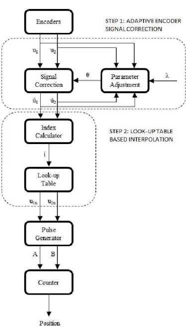
An overall flow diagram for the proposed approach is shown in Fig. 1. In this figure, signal correction and interpolation steps are labeled as step 1 and step 2, respectively. The correction step takes the encoder signals u1 and u2 and generates signals û1 and û2
as corrected quadrature signals. In order to compensate the errors in u1 and u2, a set of correction parameters θ is calculated using
RLS with exponential forgetting and resetting in the parameter adjustment block and fed into the signal correction block. Here, our parameter adjustment rule uses the current encoder signals u1
and u2 and corrected signals û1 and û2 from previous iteration. λ is
the forgetting factor or discounting factor. When the correction step is completed, index calculator generates index, i, for signals to obtain the corresponding high-order sinusoid values, u1n and u2n,
from the look-up table. The look-up table is constructed using the correct values of high-order sinusoids since the corrected signals coming from the Step 1 are calculated with sufficient precision through the adaptive correction scheme. Therefore, the look-up table can be easily generated offline without requiring high computational effort. Using high-order sinusoids, pulse generator generates quadrature binary pulses A and B without requiring high-precision ADCs. Finally, position value is calculated by detecting zero crossings of high-order sinusoids.
FIGURE 1. GENERAL FLOW DIAGRAM OF THE PROPOSED APPROACH
Step 1: Adaptive Encoder Signal Correction
Before the interpolation step, it is crucial to correct the errors in the original encoder signals to prevent high interpolation errors. Common errors affecting the quadrature encoder signals are amplitude difference, mean offsets and quadrature phase shift errors. In this paper, an adaptive approach is used to correct these errors. In some applications, it is possible to have similar error characteristics through the motion. In these cases, errors can be compensated with offline correction methods given in [5] and [7]. On the other hand, in some cases where the encoder alignment cannot be performed effectively or systems have long range of movement track, the errors change throughout the motion. In these cases, in order to obtain high-resolution, adaptive approaches may be adopted to track the errors better. For this purpose, RLS with
exponential forgetting and resetting method is developed to adjust correction parameters adaptively. In order to develop the mathematical foundation (i.e. Eq. (1) - Eq. (14)) for our proposed method, we will start with the formulation given in [7].
An ideal set of quadrature encoder signals with amplitude of A, u1i and u2i, can be expressed as
1 2 cos sin i i u A u A (1)
where α is the instantaneous phase of the signals with phase difference of π/2.
Relation between real (u1 and u2) and ideal encoder signals
(u1i and u2i) can be written as
1 1 1 2 1 2 1 ( cos( )) i u u m u A a m R (2)
where m1 and m2 are mean offset values and is the quadrature
phase shift error. In Eq. (2), R is the gain ratio (A1/A2) where A1
and A2 are amplitudes of actual encoder signals. Using Eq. (1) and
Eq. (2), a conventional least squares formulation can be obtained as shown in Eq. (3) and Eq. (4).
2 2 1 1u 2u2 3 1 2u u 4 1u 5u2 1 (3) where 2 2 2 2 2 1 1 1 1 2 1 2 2 2 2 1 3 1 4 1 1 2 5 1 2 1 ( cos 2 sin ) 2 sin 2 ( sin ) 2 ( sin ) A m R m Rm m R R m Rm R Rm m (4)
Although it is possible to calculate θi (i=1,2,…,5) constants
offline using least squares, in this paper RLS with exponential forgetting is used to calculate θi’s adaptively. For this purpose, an
equivalent of Eq. (3) can be written as shown in Eq. (5).
1 1 2 2 3 3 4 4 5 5 ( ) ( ) ( ) ( ) ( ) ( ) ( ) ( ) ( ) ( ) 1 ( ) ( ) 1 T or t t t t t t t t t t t t (5)
where superscript T denotes transpose of a matrix, t is time index, θi’s are parameters to be determined and
i’s are known functionsdepending on actual encoder signal values. Then, the parameter update and regressor vectors given in Eq. (6) are obtained.
FIGURE 2. ENCODER SIGNAL PARAMETERS RECORDED THROUGH THE 120mm MOTION OF THE SINGLE AXIS
SLIDER 2 2 1 2 1 2 1 2 1 2 3 4 5 ( ) [ ( ), ( ), ( ) ( ), ( ), ( )] ( ) [ ( ), ( ), ( ), ( ), ( )] T T t u t u t u t u t u t u t t t t t t t (6)
The aim of RLS with exponential forgetting and resetting is to determine the parameters so that Eq. (5) should be satisfied as closely as possible. For this purpose, a loss function given in Eq. (7) is determined so that the chosen θ should minimize its value.
2 1 1 ( , ) (1 ( ) ) 2 t t k T k V t k
(7)where k is index and λ is forgetting factor such that 0 . By 1 adjusting the value of λ, effects of old data to the loss function is determined so that most recent data is given unit weight whereas old data is weighted by λs, where s is number of time units passed
from the old data.
Then, the recursive parameter adjustment law can be obtained as follows 1 ( ) ( 1) ( )(1 ( ) ( 1)) ( ) ( 1) ( )( ( ) ( 1) ( )) ( ) ( ( ) ( )) ( 1) / T T T t t K t t t K t P t t t P t t P t I K t t P t (8)
where I is identity matrix and P is a non-singular matrix which can be chosen as
P
I
,
is a large number.For simplicity, time index t is omitted from this point, although each correction parameter is time-varying. Calculating the θi’s using the Eq. (8), the correction parameters (A1, R, m1, m2
and
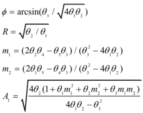
) can be obtained in terms of θi’s using Eq. (4) as3 1 2 2 1 2 1 2 4 5 3 3 1 2 2 2 1 5 4 3 3 1 2 2 2 2 1 1 2 2 3 1 2 1 2 1 2 3 arcsin( / 4 ) / (2 ) / ( 4 ) (2 ) / ( 4 ) 4 (1 ) 4 R m m m m m m A (9)
As a result, the corrected quadrature signals can be calculated using the correction parameters obtained in Eq. (9) as follows
1 1 1 1 2 1 1 2 2 1 1 ( ) 1 (( ) sin ( )) cos û u m A û u m R u m A (10)
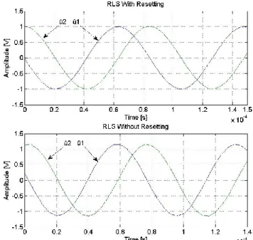
Using this method, the correction parameters are adjusted in each iteration recursively considering the effects of parameter values from previous iterations. Hence, slow changes in the parameters can be covered effectively. In Fig. 2, changes in the signal amplitude, gain ratio, mean offsets, and phase shift errors recorded through the 120mm motion of our single axis slider are shown. For short range movements (less than hundreds of micrometers), parameters can be assumed to change smoothly and continuously. However, as it can be observed in Fig. 2, they may change more dramatically for long range motions. For this case, a standard RLS with exponential forgetting cannot estimate the parameters very well. Hence, in long range motions, resetting is used to cover the significant parameter changes. For this purpose, the matrix P in the RLS algorithm given in Eq. (8) is reset periodically to its initial value ofI. As a result of resetting, the parameter estimate is updated with larger step size so that the significant changes in the parameters can be estimated well since the gain K(t) in Eq. (8) gets larger [15]. In Fig. 3, corrected encoder signal data obtained through the end of 120mm motion of slider is given for RLS with resetting and without resetting cases. It is obvious that a better correction of the encoder signals is accomplished using RLS with resetting where long range motion is the focus of interest. As shown in the Fig. 3, when there is no resetting of matrix P in the RLS algorithm, corrected signals still contain amplitude, mean offset and phase shift errors at the end of long range motions. The amplitude error for no resetting case is around 14% and 16%. Mean offset errors can reach up to 0.1V and phase shift error is about 2.5-3 degrees. Although the phase shift error seems small, when high-resolution measurements are concerned, it is not acceptable. Moreover, these errors will be amplified when an interpolation method is applied to obtain high-resolution. Illustration of the encoder signals obtained before and after correction using RLS with exponential forgetting and
FIGURE 3. CORRECTED ENCODER SIGNALS USING RLS WITH AND WITHOUT RESETTING
resetting is given in Fig. 4. In order to illustrate the quadrature phase shift of the corrected signals more clearly, variation of amplitude of corrected signals between 0 and π/2 radians are given Fig. 5. As it can be observed in this figure, corrected signals have a phase difference of π/2 as desired.
Step 2: Signal Interpolation
Calculation of higher order sinusoids can be a tedious operation based on general formulations such as given in [5]. This may reduce accuracy and the real time performance of the interpolation process. In our method, we use a look-up table based interpolation method for mapping of original encoder signals to high-order sinusoids at high process speeds. For this purpose, a quick access look-up table is formed offline. The look-up table used in this paper directly uses the actual mathematical values of high-order sinusoids since the corrected signals coming from the adaptive signal correction step are sufficiently close to the real sinusoidal signal values. Moreover, as mentioned previously, signal characteristics changes significantly in long ranges. Hence, it is much more practical to use the mathematical values of high-order sinusoids. Also, generation of the look-up table in this method becomes very easy and the same look-up table is applicable to different encoders or operation conditions.
In the interpolation step, the index calculator shown in Fig. 1, takes the values of corrected signals, û1 and û2, as inputs and
generates an index number, i. Using this number as an addressing data, the values of nth order sinusoids, u
1n and u2n, corresponding
to û1 and û2 are obtained from the quick access look-up table.
FIGURE 4. CORRECTED AND ORIGINAL ENCODER SIGNALS
FIGURE 5. VERIFICATION OF QUADRATURE PHASE DIFFERENCE BETWEEN CORRECTED SIGNALS
Construction of Look-up Table and Generation of Index Numbers. For our research, we construct our look-up table by dividing each octants (i.e. interval of π/4 radians) of a set of nth order sinusoidal signals, cos( )na and sin( )na , into N samples leading 8N samples over one period of a high-order sinusoids. Then, values of these samples are stored in the look-up table prior to the process. A generic look-up table for an nth order
interpolation is given in Tab.1. In this table, i denotes the index number generated by index calculator for û1 and û2.
After the look-up table is constructed, the index number should be calculated for mapping of corrected signals to the nth
order sinusoids. As also observed in [5], when the index calculation is based on just one signal, û1 or û2, poor resolution
will be obtained around û 1 1or û 2 1due to the highly nonlinear relationship between amplitude and angle α of sinusoidal signals. Although it is sufficient to use high N values to solve this problem, it will also increase the size of look-up table. Hence, index number may be calculated using the one of the signals, û1 or
TABLE 1. A GENERIC LOOK-UP TABLE
Index cos( )na sin( )na
0 1 0 1 cos( ) 8 n N sin( ) 8 n N 2 cos( ) 4 n N sin( ) 4 n N : : : i cos( ) 8 ni N sin( ) 8 ni N : : : 8N 1 0
û2, which is outside of that poor resolution region. Defining the
poor resolution region as
1 2 sin( ) 4 sin( ) 4 û û (11)
the index can be calculated by using almost linear relationship between amplitude and angle α outside of these regions in combination with the signs and magnitudes of the signals û1 and
û2. Signs and magnitudes of the signals are only used to find the
correct octant of the current angle. For example, for 0 a / 4,
1
( ) 0
sign û and û2 sin( / 4) . Since û2 is in the poor resolution
area mentioned above, it is suitable to use the value of û1 to
calculate the index value. Using the linear relationship between amplitude of signal û1 and the angle, it can be calculated as
1 sin( / 4) û N i (12)
Similarly, for / 4 a / 2, sign û ( )2 0 and û1
sin( / 4) . Hence, since û2 is at outside of the poor resolution region, it can beused in the calculation leading the index value of 2 2 sin( / 4) û N i N (13)
However, using Eq. (12), Eq. (13) and similar ones given in Tab.2 for the other octants of sinusoids, obtained index numbers may not be integers. Therefore, calculated index values should be rounded to the closest integer values while implementing the above method in order to reach the correct value in the look-up table.
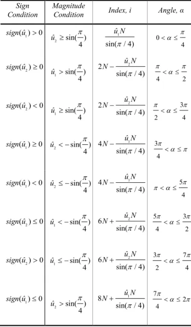
TABLE 2. INDEX CALCULATION TABLE Sign
Condition
Magnitude
Condition Index, i Angle, α 1 ( ) 0 sign û 2 sin( ) 4 û 1 sin( / 4) û N 0 4 2 ( ) 0 sign û 1 sin( ) 4 û 2 2 sin( / 4) û N N 4 2 2 ( ) 0 sign û 1 sin( ) 4 û 2 sin( / 4)2 û N N 3 2 4 1 ( ) 0 sign û 2 sin( ) 4 û 4 1 sin( / 4) û N N 3 4 1 ( ) 0 sign û 2 sin( ) 4 û 4 1 sin( / 4) û N N 5 4 2 ( ) 0 sign û 1 sin( ) 4 û 6 2 sin( / 4) û N N 5 3 4 2 2 ( ) 0 sign û 1 sin( ) 4 û 6 2 sin( / 4) û N N 3 7 2 4 1 ( ) 0 sign û 2 sin( ) 4 û 1 8 sin( / 4) û N N 7 2 4
In Tab. 2, there are two conditions to define the index. These are called as sign and magnitude conditions. Index is calculated following the similar procedure as in the above examples. Since the table is constructed by considering only the signs and magnitudes of the available encoder signals, it is easier to understand and implement in real time applications compared to the ones mentioned in the literature. It also serves as a quick access tool for the look-up table. Moreover, round off error is minimized by eliminating extra index numbers proposed in [5]. Using Tab. 2 for calculation of index and obtaining the corresponding values from the look-up table, nth order sinusoidal
signals can be obtained. An example interpolation results for n=25 is given in Fig. 6. In the interpolation, N is chosen to be 1000. Considering the results shown in Fig. 6, it is obvious that high-order sinusoids can be obtained effectively using the presented
FIGURE 6. INTERPOLATION RESULTS FOR n=25
FIGURE 7. VARIATION OF INDEX NUMBER (n=25) correction and interpolation methods. Moreover, calculated index number, i, corresponding to the corrected signals, û1 and û2, is
given in Fig. 7. In this figure, amplitudes of sinusoidal signals are set to 8000 deliberately to show the relationship between signal amplitudes and index clearly. Expectedly, index number varies from 0 to 8000 (8N) linearly in one period of signals. Linear relationship shown in this figure also illustrates the effectiveness of the proposed interpolation method. See the experiments section for more detailed experiments and results for the proposed interpolation method.
Binary Pulse Generation
In order to use the interpolated encoder signals, u1n and u2n, as
position information in a system, quadrature signals should be converted to the binary pulses. Then, the position information can be derived by counting the zero-crossings of these binary pulses. Although it is possible to use extra hardware for this purpose, it can be accomplished in software easily by using the following equations 1 1 2 2 1 1 1 1 n n n n if u A if u if u B if u
(14)where A and B are binary pulses as illustrated in Fig.1. In the Eq. (14), ε is the small threshold value. This value should be chosen
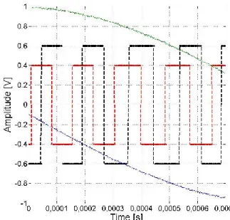
FIGURE 8. BINARY PULSES OBTAINED WITH n=25 considering the noise level of the interpolated signals coming from the interpolation step. With the proper selection of this number, undesired zero crossings can be eliminated although encoder signals contain significant amount of error.
In Fig. 8, binary pulses generated using Eq. (14) are shown. In this figure, corrected (û1 and û2) analog signals are also given.
Interpolation is conducted for n=25 and threshold value, ε, is chosen to be 0.05V. In order to prevent confusion, amplitudes of binary pulses are set to 0.4 and 0.6 for A and B, respectively. EXPERIMENT RESULTS
In this section, several experiments conducted on a single axis and two axis slider systemsare given to illustrate the performance of the proposed adaptive correction and interpolation methods.
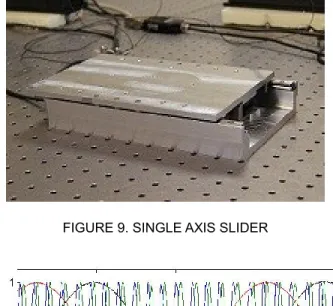
In Fig. 9, single axis slider testbed on which the experiments conducted is shown. Two axis experiments are also performed on a system which is obtained by assembling two identical sliders on top of each other perpendicularly. Each slider is driven by a permanent magnet linear motor. As a position sensor, they include Heidenhain LIP481R linear optical encoder with the original resolution of 1 micrometer. Travel range of the sliders is 120mm.
Raw signals collected using the linear encoder attached on the slider. Then, the proposed adaptive correction and look-up table based interpolation methods are used to obtain high resolution. Figure 10, Fig. 11 and Fig. 12 show the interpolation results with n=16, n=50 and n=100, respectively. In Fig. 6, interpolation with n=25 is also given. In these figures, interpolated signals and corrected signals are shown to illustrate the performance of the presented method. All of these processes is accomplished with N=1000 samples per octant. As it can be observed from these figures, sensitivity to noise increases with increasing interpolation number. Hence, as mentioned previously, it is very important to
FIGURE 9. SINGLE AXIS SLIDER
FIGURE 10. INTERPOLATION RESULTS FOR n=16 select a proper threshold value, ε, for binary pulse generation. With the proper selection of ε, undesired switching due to the interpolation noise can be eliminated. Therefore, resulting position value will not be affected from the noise generated during the interpolation. On the other hand, in order to achieve high interpolation values, noise in the encoder signals should be minimized by proper shielding, grounding and etc. [5].
Positioning performance of the single axis slider system is experimented to compare the cases with and without interpolation of the encoder signals. For this purpose, same reference inputs are applied to the system. A conventional PID controller is used as a feedback controller. For the interpolation case, n=50 is used so that the resolution of the measured position is 20nm. In Fig. 13, performance of the system for the reference input of 5 micrometers is illustrated. In order to compare the tracking errors, the reference input is given as an S-curve. From this figure, it is obvious that the positioning precision is increased significantly considering the focus of interest is micro/nano-meter level positioning.
Also, the method presented here is successfully implemented on a two axis positioning system achieving high-tracking and contouring accuracy. In Fig.14, reference input trajectory applied to the two-axis positioning system is given. Shape of the input is designed to observe tracking and contouring performance of the system. Figure 15 shows the resulting tracking and contouring
FIGURE 11. INTERPOLATION RESULTS FOR n=50
FIGURE 12. INTERPOLATION RESULTS FOR n=100
FIGURE 13. TRACKING PERFORMANCE OF THE SINGLE AXIS SLIDER
errors for the cases with no interpolation and interpolation with n=40. Here, contour error is defined as the distance between actual position and the nearest position on the contour. For this experiment, cross coupled control with iterative learning is implemented as controller. When there is no encoder signal interpolation, both tracking and contouring errors are at micrometer scale. However, when the encoder signal interpolation is employed, root mean square (RMS) of contouring error, x-axis and y-axis tracking errors are obtained as 27nm, 21nm and 66nm, respectively. Details on this study can be found in [16].
FIGURE 14. REFERENCE INPUT TRAJECTORY
FIGURE 15. TRACKING AND CONTOURING PERFORMANCE OF TWO-AXIS POSITIONING SYSTEM
CONCLUSION
In this paper, a new approach to obtain high resolution position information from original encoder signals is proposed. In this approach, correction of signal errors including amplitude difference, mean offsets and quadrature phase shift errors is accomplished adaptively by using recursive least squares with exponential forgetting and resetting. With the implementation of this method, even dynamically changing errors are effectively compensated. Then, a look-up table based interpolation method is proposed for mapping of original sinusoids to high-order ones. Since the table is constructed offline, computational effort is kept minimal. Converting the high-order sinusoids into binary pulses,
high resolution position information is obtained. Effectiveness of the proposed method is illustrated with the experimental results. Using the proposed method, up to 100 interpolations have been accomplished successfully. As a result, 10nm resolution is obtained with an optical encoder having 1µm original resolution. Minimizing the electrical noise, the number of interpolation, hence, the resolution can be further increased. Moreover, applicability of the proposed method is proven with the implementation on single and two-axis positioning devices without requiring any extra hardware. Combining our interpolation method with a suitable controller, tracking performance of both systems are increased significantly [16]. Less than 30nm contouring error is accomplished for two axis positioning system.
Although nanometer level resolutions are accomplished with the presented interpolation method, it is sensitivity to noise cannot be ignored for high interpolation numbers (>100). Hence, in future, sensitivity to noise is to be reduced to obtain higher resolution values.
ACKNOWLEDGMENTS
This research is sponsored by Scientific and Technical Research Council of Turkey (TUBITAK) through Project No: 110M251. Authors also would like to thank Dr. Sinan Filiz and undergraduate students Ersun Sozen and Oytun Ugurel for their support on mechanical design of the slider.
REFERENCES
[1] Devasia, S., Eleftheriou, E. E., and Moheimani, R., 2007. “A Survey of Control Issues in Nanopositioning”. IEEE Transactions on Control Systems Technology, Vol.15, No15, pp.802-823.
[2] Manske, E., Hausotte, T., Mastylo, R., Machleidt, T., Franke, K., and Jager, G., 2007. “New Applications of the Nanopositioning and Nanomeasuring Machine by Using Advanced Tactile and Non-tactile Probes”. Measurement Science and Technology, 18(2), pp. 520-527.
[3] Lihua, L., Yingchun, L., Yongfeng, G., and Akira, S., 2010. “Design and Testing of a Nanometer Positioning System”. Journal of Dynamic Systems, Measurement, and Control, 132(2), pp. 02011-6.
[4] Pang, C. K., Guo, G., Chen, B. M., and Lee, T. H., 2006. “Self-sensing Actuation for Nanopositioning and Active-mode Damping in Dual Stage HDDs”. IEEE/ASME Transactions Mechatronics, 11(3), pp. 328-338.
[5] Tan, K. K., Zhou, H. X., and Lee, T. H., 2002. “New Interpolation Method for Quadrature Encoder Signals”. IEEE Transactions on Instrumentation and Measurement, Vol. 51, No5, Oct., pp.1073-1079.
[6] Tan, K. K., Tang, and K. Z., 2005. “Adaptive Online Correction and Interpolation of Quadrature Encoder Signals Using Radial Basis Functions”. IEEE Transactions on Control Systems Technology, Vol. 13, No3, May, pp. 370-377.
[7] Heydemann, P. L. M., 1981. “Determination and Correction of Quadrature Fringe Measurement Errors in Interferometers”. Applied Optics, Vol. 20, No19, Oct. [8] Birch, K. P., 1990. “Optical fringe subdivision with
nanometric accuracy”. Precision Engineering, Vol. 12, No.4, Oct..
[9] Balemi, S., 2005. “Automatic Calibration of Sinusoidal Encoder Signals”. Proc. 16th IFAC World Congr,. Prague, Czech Republic, Jul..
[10] Hoang, H. V., Jeon, J. W., 2011. “An Efficient Approach to Correct the Signals and Generate High-Resolution Quadrature Pulses for Magnetic Encoders”. IEEE Transactions on Industrial Electronics, Vol. 58, No.8, Aug..
[11] Cheung, N. C., 1999. “An Innovative Method to Increase the Resolution of Optical Encoders in Motion Servo Systems”. Proc. IEEE Int. Conf. Power Electronics and Drive Systems, Hong Kong, Jul., pp. 797-800.
[12] Madni, A. M., Jumper, M., and Malcolm, T., 2001. “An Absolute High-Performance, Self-Calibrating Optical Rotary
Positioning System”. Proc. IEEE Aerospace Conf., Vol.5, Mar., pp. 2363-2373.
[13] Le, H. T., Hoang, H. V., and Jeon, J. W., 2008. “Efficient Method for Correction and Interpolation Signal of Magnetic Encoders”. Proc. IEEE International Conference on Industrial Informatics, Jul., pp. 1383-1388.
[14] Hoseinnezhad, R., Bab-Hadiashar, A., and Harding, P., 2007. “Calibration of Resolver Sensors in Electromechanical Braking Systems: A Modified Recursive Weighted Least-Squares Approach”. IEEE Trans. Ind. Electron., Vol.54, No.2, Apr., pp. 1052-1060.
[15] Astrom, K. J., and Wittenmark, B., 1995. Adaptive Control, 2nd ed..Dover Publications, Mineola, NY, Chap. 2, pp.42-56.
[16] Gecer Ulu, N., Ulu, E. and Cakmakci, M., 2012. “Learning Based Cross-Coupled Control for Multi-axis High Precision Positioning Systems”. ASME Dynamic Systems and Control Conf. (DSCC2012), Ft. Lauderdale, FL, Oct..