Estimation of
and
Communication
Parameters of Ionosphere
-Layer Using
GPS Data and IRI-Plas Model
Umut Sezen, Oktay Sahin, Feza Arikan, and Orhan Arikan
Abstract— -layer is the most important and characteristic layer of the ionosphere in the propagation of high frequency (HF) waves due to the highest level of conductivity in the propagation path. In this study, the relation of Total Electron Content (TEC) with the maximum ionization height and the critical frequency of -layer are investigated within their defined parametric range using the IRI model extended towards the plasmasphere (IRI-Plas). These two parameters are optimized using daily observed GPS-TEC (IONOLAB-TEC) in an iterational loop through Non-Linear Least Squares (NLSQ) optimization while keeping the physical correlation between and parameters. Optimization performance is examined for daily (24-hour) and hourly TEC optimizations separately. It is observed that hourly TEC optimization produces results with much smaller estimation errors. As a result of the hourly optimization, we obtain the hourly and estimates as they are the optimization parameters. Obtained and estimates are compared with the ionosonde estimates for various low, middle and high latitude locations for both quite and disturbed days of ionosphere. The results show that and estimates obtained from IRI-Plas optimization (IRI-Plas-Opt) and ionosonde are very much in agreement with each other. These results also signify that IRI-Plas provides a reliable background model for ionosphere. With the proposed method, it is possible to build a virtual ionosonde via optimization of IRI-Plas model using the observed TEC values.
Index Terms—foF2, GPS, hmF2, IONOLAB, IRI-Plas, TEC, vir-tual ionosonde.
I. INTRODUCTION
I
onosphere is the layer of the atmosphere that lies between 60 km and 1000 km above Earth surface and has a great importance in high frequency (HF) and satellite communica-tions because of its electrical and ionic structure. The ionization characteristics and electron density distribution vary accordingManuscript received October 10, 2012; revised May 31, 2013; accepted July 01, 2013. Date of publication July 29, 2013; date of current version October 02, 2013. This work was supported in part by TUBITAK EEEAG Grants 109E055 and 110E296.
U. Sezen and F. Arikan are with the Department of Electrical and Electronics Engineering, Hacettepe University, Ankara 06532, Turkey.
O. Sahin is with the Department of Avionics and Naval Systems Design, Aselsan Inc. Microelectronics, Guidance and Electro-Optics Division, Ankara 06750, Turkey.
O. Arikan is with the Department of Electrical and Electronic Engineering, Bilkent University, Ankara 06800, Turkey.
Color versions of one or more of the figures in this paper are available online at http://ieeexplore.ieee.org.
Digital Object Identifier 10.1109/TAP.2013.2275153
to the location on Earth, time, solar, geomagnetic and seismic effects. Ionosphere consists of three distinct layers, namely , and . layer is normally divided into and layers. -layer, having the highest electron density, is the most stable layer for HF communications and it has major importance in satellite communications [1]. -layer models can be found in various studies including but not limited to [2]–[5]. The critical parameters of -layer can be estimated using ionosondes [6]–[8]. -layer model estimates are also investigated in the context of HF communications in [9] and [10]. In [10], HF channel electromagnetic parameters are estimated via ray tracing using a modified International Reference Ionosphere (IRI) model.
Many experimental and theoretical models—including but not limited to TIEGCM, GTIM, and SUPIM [11]—are de-veloped to obtain a realistic physical structure of ionosphere. Among these models, the most complete and widely used one is the IRI model [5], [12]. IRI is an international project sponsored by the Committee on Space Research (COSPAR) and the International Union of Radio Science (URSI). For a given location, time and date, IRI provides the estimates of the electron density, electron temperature, ion temperature, and ion composition based on the monthly averages (www.iri.org). In a recent study, IRI model is extended to include plasmas-phere (IRI-Plas) up to 20,000 km corresponding to the height of Global Positioning System (GPS) satellites [13], [14]. In IRI-Plas, TEC estimates can be also provided externally as input for the proper scaling of topside and plasmasphere exten-sions. In this study, TEC values are the IONOLAB-TEC [15], [16] estimates obtained from GPS data. The goal of this study is to optimize IRI-Plas with the IONOLAB-TEC values using the two IRI-Plas parameters and while considering the physical correlation between these two parameters in a well-designed iterative optimization loop. With the proposed method, it is aimed to obtain more realistic ionospheric com-munication parameters with a high resolution representation of time and location on Earth. This study will extend the single dimensioned ionospheric structure characterized only by TEC values to a three dimensional structure by adding and estimates, for better characterization of HF channel. Preliminary results of IRI-Plas optimization are presented in [17]–[20], respectively. IRI-Plas optimizations with TEC input and without TEC input are considered in [17] and [19], respec-tively, while the physical relationship between the and parameters are not taken into account. [19] added the physical relationship between the and parameters
tion structure used for the estimation of -layer parameters is explained in Section IV. Later, Section V discusses the opti-mization strategy and presents the optiopti-mization results together with the obtained and estimates.
II. IONOLAB-TEC METHOD
In this study, IONOLAB-TEC (www.ionolab.org) is used as the GPS-TEC data. IONOLAB-TEC [15], [16], [21], [22] com-bines data from all the GPS satellites that are above 10 ele-vation angle (horizon limit) of the GPS station with a temporal resolution of 30 seconds. The method calculates VTEC (Vertical Total Electron Content) per satellite and combines them using a weighting function based on satellite positions which reduces the contamination caused by multipath effects [16], [21]. The re-ceiver differential code biases are estimated using IONOLAB-BIAS method described in [15]. IONOLAB-TEC estimates are robust, reliable and accurate, and they can be used with any single GPS station either in IGS1or EUREF2network.
III. IRI-PLAS MODEL ANDMODELPARAMETERS
IRI-Plas model [13], [14] being an improved version of the IRI model [5], [12], [23] with the plasmasphere extension [24] is a climatic and empirical model of ionosphere that can be up-dated with different observational data sources. In IRI-Plas, the region of interest has been extended to plasmasphere, i.e. 20,000 km. Ion and electron density distributions and TEC estimates along the local zenith axis can be obtained using this model. The TEC estimates (in topside and plasmasphere regions) can be scaled by providing observed (or measured) TEC inputs. Some of the model inputs, such as Sun Spot Number (SSN) and ge-omagnetic coordinates do not change for a given day and are kept constant in the used data set. Some of the parameters are option selection flags used for deciding internal sub-models and input-output configuration settings. Output parameters of the model are provided for each layer of ionosphere as TEC esti-mates and related layer-critical values.
During the sunlit hours, all ionosphere layers are available, but when ionization effect of Sun disappears at night, -layer becomes the predominant layer in spite of a decrease in peak electron density [4], [10]. Two main characteristic parameters of this layer are the maximum ionization height (km) and the critical frequency (MHz). Only electromagnetic sig-nals above a critical frequency level can traverse the ionosphere and propagate into outer space. Signals with lower frequencies are refracted and reflected. Therefore, is very important in
1The International GNSS (Global Navigation Satellite Systems) Service 2IAG (International Association of Geodesy) Reference Frame
Sub-Commis-sion for Europe
Fig. 1. IRI-Plas model with input and output parameter sets.
radio communications [1], [10]. IRI-Plas model estimates crit-ical frequency and height values by analyzing its preset coeffi-cient matrices.
In this study, -layer critical height and frequency input parameters are examined hourly for any selected day, with and without the scaling effect of observational TEC given as an external input to IRI-Plas. Related input
parame-ters are represented with , , and
for the -th hour of day during this study. Other non-optimized parameters such as configuration setting flags, latitude, longi-tude, date, time, daily SSN and index (SSN and index are database inputs independent of user entries) are represented with vector, as shown in Fig. 1. Produced model
esti-mates are represented with , , and
other layer estimates are defined as . So, final estimates vector is given below, as
(1) where denotes the transpose of a vector or matrix.
IRI-Plas model without TEC input is defined as
(2) and IRI-Plas model with TEC input is defined as
(3) where represents the measured (or observed) TEC value for the -th hour of the day obtained by IONOLAB-TEC. It is aimed to get a more realistic estimation vector, by using a well-designed optimization loop.
IV. IRI-PLAS OPTIMIZATIONDESIGN
Correlation between and parameters and the scaling effect of TEC input need to be investigated before moving on to the optimization design. As a first step, output of IRI-Plas is plotted for different values of for a quite day (15 October 2008) and location (unpg station
Fig. 2. Physical correlation characteristics of and for a quiet day (unpg, 15 October 2008).
correlation between and parameters. As seen in Fig. 2, IRI-Plas — correlation is high during day hours, and less for night hours.
Later, for a selected quite day (15 October 2008 and unpg sta-tion), IRI-Plas input parameter-set affecting TEC estimates are investigated in their defined parametric range as shown in Fig. 3 and Fig. 4. In order to achieve this, root-mean-squared (RMS) error between IRI-Plas TEC estimates and IONOLAB-TEC values is calculated separately for and variations. Initially, dependency of IRI-Plas TEC estimates to is investigated, where is taken as the default IRI-Plas daily average, , for the selected location and day. Hence, for a given day the average frequency , and
average daily TEC error are given by
(4) and
(5) respectively. In the above equations, represents the hour of
the day and is given by
(6) Here, is varied between 150 km and 600 km in steps of 50 km. Results are shown on Fig. 3. It is seen from Fig. 3(a) that the average error is a parabolic curve. Fig. 3(b) shows the variation of the where the emphasized (bold) curve in the middle indicates the observed IONOLAB-TEC, . Also Fig. 3(c) shows the variation of the which is obtained by using the observed TEC as the input to IRI-Plas, i.e.,
(7) where the emphasized (bold) curve in the middle indicates the observed IONOLAB-TEC, . The scaling effect of top-side and plasmasphere regions of IRI-Plas with TEC input is
Fig. 3. IRI-Plas single parameter search on 15 October 2008 at unpg: (a) Daily RMS error (without TEC input) (b) Daily -TEC variation without TEC input (c) Daily -TEC variation with TEC input.
clearly seen in Fig. 3(c), showing that the effect of vari-ations on TEC output is greatly reduced.
Similarly, while investigating dependency of IRI-Plas TEC estimates to , is taken as the default IRI-Plas daily average, for the selected location and day. Hence, for a given day the average frequency , and average daily TEC error are given by
(8) and
(9)
respectively. Here, is given by
(10) Here, is varied between 2 MHz and 9 MHz in steps of 1 MHz. Results are shown on Fig. 4. It is seen from Fig. 4(a) that the average error is also a parabolic curve. Fig. 4(b) shows the variation of the where the emphasized (bold) curve in the middle indicates the observed IONOLAB-TEC, . Also Fig. 4(c) shows the variation
Fig. 4. IRI-Plas single parameter search on 15 October 2008 at unpg: (a) Daily RMS error (without TEC input) (b) Daily -TEC variation without TEC input (c) Daily -TEC variation with TEC input.
of the which is obtained by using the observed TEC as the input to IRI-Plas, i.e.,
(11) where the emphasized (bold) curve in the middle indicates the observed IONOLAB-TEC, . The scaling effect of top-side and plasmasphere regions of IRI-Plas with TEC input is clearly seen in Fig. 4(c), showing that the effect of varia-tions on TEC output is greatly reduced.
Having parabolic structures for single parameter sets, it is ex-pected that a quadratic surface will be formed for double param-eter search. So, Non-Linear Least Squares (NLSQ) optimization (with the Levenberg-Marquardt method) [25], [26] is chosen for the optimization of and parameters. The iterative optimization loop model is based on the minimization of the TEC difference between the observed and estimated TEC values as shown in Fig. 5.
IRI-Plas integrates physical correlation of critical frequency and height parameters inside its model. So, correlation is taken from the model using frequency as input and height as output shown in (12)
(12)
Fig. 5. IRI-Plas iterative optimization model.
output is used as the correlated height. A new output vector is defined as follows:
(13) where
(14)
Here and .
Error vector is defined as the combination of the
two estimation errors, and
, for each hour of day as shown below
(15) where represents the measured (or observed) TEC for the -th hour of the day obtained by the IONOLAB-TEC method. Minimizing the mean -norm square of the error
vector , i.e., minimizing ,
in an iterative loop leads to hourly optimized and parameter values.
V. DISCUSSION ON THEOPTIMIZATIONSTRATEGY ANDRESULTS
After choosing NLSQ optimization, performance evalu-ation of IRI-Plas model is investigated for different input combinations:
• running IRI-Plas with optimized parameters and TEC input, i.e.,
• running IRI-Plas only with optimized parameters (without TEC input), i.e.,
Fig. 6. IRI-Plas TEC estimation performance on 15 October 2008 at unpg.
• running IRI-Plas only with TEC input (without optimized parameters input), i.e.,
• running IRI-Plas without optimized parameters and TEC input, i.e.,
where and are the final and
values obtained at the end of hourly optimizations and they are called as the hourly and estimates, respectively.
Here, optimized parameters refer to the and pa-rameters obtained as a result of the optimization. Results are shown in Fig. 6. The normalized errors are obtained by dividing the norm of the error vectors by the norm of the observation vec-tors. In this text, normalized errors will be presented in paren-theses along with the RMS errors.
As shown in Fig. 6, using optimized parameters with and without the IRI-Plas TEC input gives the best TEC estimations with RMS errors of TECU (0.0027%) and
TECU (0.017%), respectively. Optimization algorithm which uses IONOLAB-TEC observations only for error calculations, not for IRI-Plas input, is marked with a ‘ ’ sign in Fig. 6. Run-ning IRI-Plas with TEC input only, i.e., without the optimized parameters, produces a significant RMS error of 0.70 TECU (6.45%), and shows large drifts especially during night-time as clearly seen on Fig. 6. Running IRI Model without optimization parameters and TEC input produces the highest error of 2.57 TECU (23.78%) as expected.
The scaling effect of the topside and plasmasphere regions on and parameters are shown in Fig. 3(c) and Fig. 4(c). As running IRI-Plas with TEC input reduces the ef-fect of and parameters, IRI-Plas is optimized by using only and parameters as the input parame-ters of IRI-Plas. Thus, IONOLAB-TEC values are only used in error calculations as shown in (15).
In order to observe the dependency to referenced observa-tional TEC and produce a parameter estimation error-band for and parameters, uniform random noise with an
Fig. 7. IRI-Plas optimization structure with uniform random noise.
Fig. 8. TEC estimation with uniform random noise on 15 October 2008 at unpg.
amplitude of TECU is added on the IONOLAB-TEC values used in optimization, as shown in Fig. 7.
Here, 10 different TEC vectors are produced corresponding to different noise levels as
(16)
where and is a uniform random noise with
TECU. Here TECU range indicates
an error margin during TEC measurements. These extra inputs are marked with dots viewed as vertical fluctuations around the actual hourly IONOLAB-TEC values, as shown in Fig. 8.
TEC outputs of the IRI-Plas optimization and IONOLAB-TEC values with and without noise exactly match each other as shown in Fig. 8 below.
Ionosonde RO041 located in Rome and
unpg receiver located in Perugia are se-lected for the analysis of and estimations. The approximate distance between these two locations is 147 km. Comparison of and estimates and ionosonde data for 15 October 2008, unpg EUREF receiver are given in Fig. 9 below. Here, fractured lines show the observational ionosonde data and the smoother lines with vertical fluctuations of dots show the and estimates obtained via optimization. Vertical fluctuations of dots represent the error margins of the estimations, as they are obtained for each value of .
The optimization estimates, in Fig. 9(a) and in Fig. 9(b), match well with the ionosonde data. RMS differ-ences for and estimates are found to be 31.42 km (12.8%) and 0.70 MHz (14.3%), respectively. The difference in the values are higher during night hours as seen in
Fig. 9. Comparison of and estimates with ionosonde data for
unpg-RO041 on 15 October 2008: (a) , (b) .
Fig. 9(a). Also for values shown in Fig. 9(b), a sudden jump in the ionosonde data is seen between 10:00–12:00 UT which increases the matching error. This jump may be due to a local disturbance in the ionosphere that is not recorded as a ge-omagnetic storm, or due to a measurement error. Due to these sudden and short duration variabilities that may occur in instan-taneous data, ionospheric scientists use hourly or monthly run-ning mean and median values before they include the measure-ment data into their models.
The optimization algorithm is also tested for loca-tions in higher latitudes. The results for wroc IGS
re-ceiver located in Wroclaw and the
nearest ionosonde of JR055 located in
Juliusruh/Rugen are provided in Fig. 10. The approximate distance between these two locations is 460 km.
Similarly, in Fig. 10, fractured lines show the JR055 ionosonde data and the smoother lines with vertical fluctuations
of dots show the and estimates obtained via
optimization. RMS differences for and estimates are found to be 30.48 km (11.8%) and 0.37 MHz (9.3%), re-spectively. The difference in the values are higher in the night-time as seen in Fig. 10(a). Both and plots indicate that nearly all ionosonde data lie within the estimation error-bands which correspond to approximate errors of 1 TECU made in TEC measurements.
In Fig. 11, the comparison is provided for karr IGS
re-ceiver located in Karratha and LM42B
ionosonde located in Learmonth. The
approximate distance between these two locations is 337 km. Here, fractured lines are the observational ionosonde data and the smoother lines with vertical fluctuations of dots are the and estimates obtained via optimization. Here,
RMS differences for and estimates are found
to be 13.4 km (4.8%) and 0.32 MHz (6.7%), respectively. Fig. 11(a)–(b) shows that ionosonde data and our and estimates are very much in agreement with each other.
Fig. 10. Comparison of and estimates with ionosonde data for
wroc-JR055 on 15 October 2008: (a) , (b) .
Fig. 11. Comparison of and estimates with ionosonde data for
karr-LM42B on 15 October 2008: (a) , (b) .
The performance of the proposed algorithm is evaluated for a longer period in 2008 for LM42B ionosonde and karr GPS stations. LM42B ionosonde data were missing before 21 Au-gust 2008 and karr GPS receiver data were missing for some days in December. So, the remaining four-month data are pro-cessed with the proposed optimization method with an RMS error of TECU and the results are shown (as a scatter plot) in Fig. 12(a)–(b) and summarized in Table I. The figures indicate that estimates cover most of the scat-tering of the ionosonde data, and estimates show a strong underlying trend, probably which the IRI-Plas model imposes. Although maximum errors can be high as indicated in Table I, RMS errors of 24.31 km and 0.83 MHz are actually in an acceptable range. For example, [27] reports a similar order of
Fig. 12. Long term comparison of and estimates with ionosonde data for karr-LM42B (21 August 2008–23 December 2008): (a)
, (b) .
TABLE I
LONGTERMPERFORMANCEANALYSIS OF THEOPTIMIZATIONMETHOD
(21 AUGUST2008–23 DECEMBER2008)
mismatch between two measurement systems, a MU radar and ionosonde, in terms of values.
The proposed method is also tested for disturbed days of ionosphere corresponding to a geomagnetic storm. The dates, 29 October 2003 and 8 October 2012 are chosen for analysis. The former date is a well-known strong geomagnetic storm date. The latter date is a moderate geomagnetic storm date. The ionosonde and GPS stations are chosen according to data availability and location distance. On 29 October 2003,
ionosonde AT138 located in Athens and orid
receiver located in Ohrid are selected for
the analysis of and estimations. The approximate distance between these two locations is 423 km.
Fig. 13. IRI-Plas TEC estimation performance on 29 October 2003 at orid.
Fig. 13 shows that plain IRI-Plas TEC values (indicated with circles) are much lower than the observed IONOLAB-TEC values, giving an RMS error of 66.8 TECU (39%). However, optimization results (indicated with squares) perfectly match with the IONOLAB-TEC values (indicated with dots and line)
with and RMS error of TECU. Resulting and
estimates are shown in Fig. 14(a)–(b), respectively. The mismatch is high in with an RMS difference of 294 km (18.13%). estimates follow the trend of the ionosonde values closely with an RMS difference of 6.24 MHz (15%).
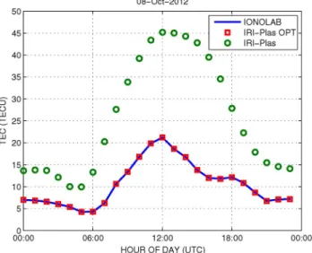
On 8 October 2012, Ionosonde RL052
lo-cated in Chilton and hert receiver located in Hailsham are selected for the analysis of and esti-mations. The approximate distance between these two locations is 140 km. Fig. 15 shows that plain IRI-Plas TEC values (indi-cated with circles) are much higher than the IONOLAB-TEC es-timates, giving an RMS error of 84 TECU (146.5%). However, optimization results (indicated with squares) perfectly match with the IONOLAB-TEC values (indicated with dots and line)
with and RMS error of TECU. Resulting
and estimates are shown in Fig. 16(a)–(b), respectively. Fig. 16(a) shows that mismatch is especially higher be-tween 6 am and 12 pm. Total RMS difference is found to be 141.8 km (9.59%). In figure Fig. 16(b), estimates follow the same trend with the ionosonde values but with an RMS difference of 3.86 MHz (16.3%).
As mentioned in [6], [8], [13] and [27], ionosphere is an inhomogeneous and anisotropic region. The reflection from ionospheric layers occur over turning points and they do not resemble specular reflection. The ionosonde ‘measurements’ include this inherent ambiguity and therefore model values may agree with ionosonde computations in a wider confidence band. The critical frequency values are generally extracted from ionosonde signals using a Fourier transform based method which is more sensitive to frequency measure-ments. Therefore, the frequency estimates from ionosondes are more reliable compared to critical height estimates. As a result, IRI-Plas model coefficients, which are based on observations
Fig. 14. Comparison of and estimates with ionosonde data for
orid-AT138 on 29 October 2003: (a) , (b) .
Fig. 15. IRI-Plas TEC estimation performance on 8 October 2012 at hert.
from a wider and more complete set, provide a better agreement with ionosonde -layer critical frequency estimates.
Fig. 16. Comparison of and estimates with ionosonde data for
hert-RL052 on 8 October 2012: (a) , (b) .
VI. CONCLUSION
IRI-Plas model is optimized via and
pa-rameters in an iterative NLSQ optimization loop using the IONOLAB-TEC values in cost calculations. External TEC input is not supplied to IRI-Plas during optimization as it would force extra scaling of the topside and plasmasphere regions af-fecting and estimations. During the optimization process, physical relationship between and is preserved. IRI-Plas optimization TEC output matched exactly with the IONOLAB-TEC values. The final and parameter of the optimization are called as the and
estimates, and the specific optimization routine including IRI-Plas is called as IRI-Plas-Opt.
In this study, the and estimates are compared with the nearest ionosonde values for both quiet and disturbed days of ionosphere. It is observed that the results for the quite days are very much agreement with the ionosonde data. Although the differences in the disturbed days are higher, the results indicate that estimates follow the same trend with the ionosonde data. The proposed algorithm is tested for a four-month period, and RMS differences are found to be
24.31 km and 0.83 MHz for and values, respec-tively. The scatter bands of the IRI-Plas-Opt and ionosonde estimates are found to be mostly in agreement. However, IRI-Plas-Opt estimates demonstrate a strong underlying trend which is imposed by the IRI-Plas model. Also, estimation differences are higher during the night hours, especially for values. We expect that this may be due to IRI-Plas model structure for nighttime ionosphere or ‘measurement’ errors of ionosondes. Physically, it is more difficult to ‘measure’ values accurately than to measure values, due to the inhomogeneous and anisotropic distribution of electron density in the ionosphere. As a result, IRI-Plas favors the accuracy of
more than .
From another perspective, our results also justify the model reliability of the IRI-Plas. The proposed IRI-Plas-Opt opti-mization method allows the effective computation of and parameters of -layer using the IRI-Plas model and GPS-TEC estimates (or TEC measurements) where the ionosonde data are not available, and acts as a virtual ionosonde. The results indicate that IRI-Plas-Opt method is highly reliable especially for the quite days of ionosphere.
ACKNOWLEDGMENT
IRI-Plas executable and source code are available at http://ftp.izmiran.ru/pub/izmiran/SPIM/. Ionosonde data is available at http://spidr.ngdc.noaa.gov/. A list of geo-magnetic storms is also available at http://www.izmiran. ru/services/iweather/storm/tecstorm.txt.
REFERENCES
[1] M. Kolawole, Radar Systems, Peak Detection and Tracking. Oxford, U.K.: Newnes, 2002.
[2] J. King, J. Samuel, and G. Thuillier, “Accuracy of the CCIR F2 layer model at low and middle latitudes,” Electron. Lett., vol. 11, no. 16, pp. 366–368, 7, 1975.
[3] C. M. Rush, M. PoKempner, D. N. Anderson, F. G. Stewart, and J. Perry, “Improving ionospheric maps using theoretically derived values of foF2,” Radio Sci., vol. 18, pp. 95–107, 1983.
[4] D. Blitza, N. M. Sheikh, and R. A. Eyfrig, “Global model for the height of the F2-peak using M3000 values from CCIR(J),” Telecommun., vol. 46, no. 9, pp. 549–553, 1979.
[5] , D. Blitza, Ed., International Reference Ionosphere 1990. Greenbelt, MD: NSSDC 90-22, 1990.
[6] M. Lockwood, “Simplified estimation of ray-path mirroring height for HF radiowaves reflected from the ionospheric F-region,” IEE Proc. F,
Commun. Radar Signal Process., vol. 131, no. 2, pp. 117–124, Apr.
1984.
[7] R. D. Hunsucker, Radio Techniques for Probing the Terrestrial
Iono-sphere.. New York, NY, USA: Springer-Verlag, 1991.
[8] M. Yao, Z. Zhao, G. Chen, G. Yang, F. Su, S. Li, and X. Zhang, “Comparison of radar waveforms for a low-power vertical-incidence ionosonde,” IEEE Geosci. Remote Sens. Lett., vol. 7, no. 4, pp. 636–640, Oct. 2010.
[9] B. Barabashov, O. Maltseva, V. Rodionova, and A. Shlyupkin, “Evalu-ation of the IRI model efficiency for oper“Evalu-ational forecast of HF propa-gation conditions,” in Proc. 10th IET Int. Conf. Ionospheric Radio
Sys-tems Techniques (IRST 2006), London, U.K., Jul. 2006, pp. 253–257.
[10] Z.-W. Yan, G. Wang, G.-L. Tian, W.-M. Li, D.-L. Su, and T. Rahman, “The HF channel EM parameters estimation under a complex environ-ment using the modified IRI and IGRF model,” IEEE Trans. Antennas
Propag., vol. 59, no. 5, pp. 1778–1783, May 2011.
[11] “Guide to Reference and Standard Ionosphere Models,” ANSI, AIAA, , ser. ANSI/AIAA G, 1999, American Institute of Aeronautics and As-tronautics.
[12] D. Blitza, “International reference ionosphere 2000,” Radio Sci., vol. 36, no. 2, pp. 261–275, 2001.
[13] T. Gulyaeva, “Storm time behavior of topside scale height inferred from the ionosphere-plasmasphere model driven by the F2 layer peak and GPS-TEC observations,” Adv. Space Res., vol. 47, no. 6, pp. 913–920, 2010.
[14] T. Gulyaeva and D. Bilitza, “Towards ISO standard earth ionosphere and plasmasphere model,” in New Developments in the Standard
Model, R. Larsen, Ed. Hauppauge, NY, USA: NOVA, 2012, pp.
1–48.
[15] F. Arikan, H. Nayir, U. Sezen, and O. Arikan, “Estimation of single station interfrequency receiver bias using GPS-TEC,” Radio Sci., vol. 43, no. 4, p. RS4004, 2008, 13 pp..
[16] H. Nayir, F. Arikan, O. Arikan, and C. B. Erol, “Total electron content estimation with Reg-Est,” J. Geophys. Res., vol. 112, no. A11, p. A11 313, 2007, 11 pp..
[17] O. Sahin, U. Sezen, F. Arikan, and O. Arikan, “Determining F2 layer parameters via optimization using IRI model and IONOLAB TEC esti-mations,” in Proc. IEEE 19th Conf. Signal Process. Comm. App. (SIU
2011), Apr. 2011, pp. 630–633, in Turkish with abstract in English.
[18] O. Sahin, U. Sezen, F. Arikan, O. Arikan, and B. Aktug, “Optimiza-tion of F2 layer parameters using IRI-Plas model and IONOLAB total electron content,” in Proc. 5th Int. Conf. Recent Advances Space
Tech-nologies (RAST 2011), Jun. 2011, pp. 407–411.
[19] O. Sahin, U. Sezen, F. Arikan, and O. Arikan, “Optimization of F2 layer parameters using IRI-Plas and IONOLAB-TEC,” in Proc.
Gen-eral Assembly Scientific Symp. 2011 XXXth URSI, Aug. 2011, pp. 1–4.
[20] O. Sahin, “Estimation of HMF2 and FOF2 Communication Parame-ters of Lonosphere Using GPS Data and IRI Model,” Master’s thesis, Hacettepe University, Ankara, Turkey, Oct. 2011, in Turkish with ab-stract in English..
[21] F. Arikan, U. Sezen, O. Arikan, O. Ugurlu, and H. Nayir, “Space weather activities of IONOLAB group: IONOLAB-TEC,” in Proc.
EGU General Assembly Conf. Abstracts, D. N. Arabelos and C. C.
Tscherning, Eds., Apr. 2009, vol. 11, ser. EGU General Assembly Conference Abstracts, p. 5188.
[22] U. Sezen, F. Arikan, O. Arikan, O. Ugurlu, and A. Sadeghimorad, “On-line, automatic, near-real time estimation of GPS-TEC: IONOLAB-TEC,” Space Weather, vol. 11, pp. 1–9, 2013.
[23] D. Blitza, K. Rawer, L. Bossy, and T. Gulyaeva, “International refer-ence ionosphere—Past, present, future,” Adv. Space Res., vol. 13, no. 3, pp. 3–23, 1993.
[24] T. L. Gulyaeva, X. Huang, and B. W. Reinisch, “Plasmaspheric exten-sion of topside electron density profiles,” Adv. Space Res., vol. 29, no. 6, pp. 825–831, 2002.
[25] C. T. Kelley, Iterative Methods for Optimization, ser. SIAM Frontiers Appl. Math. 18. Philadelphia, PA, USA: SIAM, 1999.
[26] K. Madsen, H. B. Nielsen, and O. Tingleff, Methods for Non-Linear
Least Squares Problems (2nd ed.). Denmark: Informatics and
Math-ematical Modelling, Technical University of Denmark, DTU, 2004. [27] S.-R. Zhang, S. Fukao, W. L. Oliver, and Y. Otsuka, “The height of
the maximum ionospheric electron density over the MU radar,” J.
At-mosph. Solar Terr. Phys., vol. 61, pp. 1367–1383, 1999.
Umut Sezen received the B.Eng. and Ph.D. degrees
in Electronic Engineering from the University of Warwick, Coventry, U.K., in 1998 and 2003, respec-tively. During his education, he was supported by Turkish government scholarships.
Since 2004, he is with the Department of Elec-trical and Electronic Engineering, Hacettepe Univer-sity, Ankara, Turkey. His research interests include optimization, digital signal processing, wavelets and filter-bank theory.
and development, digital signal processing, modern command and control systems development.
Feza Arikan was born in Sivrihisar, Turkey, in
1965. She received the B.Sc. degree (high honors) in electrical and electronics engineering from Middle East Technical University, Ankara, Turkey, in 1986 and the M.S. and Ph.D. degrees in electrical and computer engineering from Northeastern University, Boston, MA, in 1988 and 1992, respectively.
Since 1993, she has been with the Department of Electrical and Electronics Engineering, Hacettepe University, Ankara, where she is currently a Full Professor. She is also the Director of the IONOLAB
Orhan Arikan was born in Manisa, Turkey, in
1964. He received the B.Sc. degree (high honors) in electrical and electronics engineering from Middle East Technical University, Ankara, Turkey, in 1986 and the M.S. and Ph.D. degrees in electrical and computer engineering from University of Illinois Urbana-Champaign, Urbana, IL, in 1988 and 1990, respectively.
Since 1993, he has been with the Department of Electrical and Electronics Engineering, Bilkent Uni-versity, Ankara, where he is currently a Full Professor and Department Chair. His research interests include Digital Signal Processing and applications including radar signal processing, compressive sensing and in-verse problems.
Prof. Arikan is a member of IEEE, the American Geophysical Union and URSI.