Bandit with Probabilistically Triggered Arms
Alihan H¨uy¨uk Cem Tekin
Electrical and Electronics Engineering Department Bilkent University, Ankara, Turkey
Electrical and Electronics Engineering Department Bilkent University, Ankara, Turkey
Abstract
We analyze the regret of combinatorial Thompson sampling (CTS) for the combinato-rial multi-armed bandit with probabilistically triggered arms under the semi-bandit feed-back setting. We assume that the learner has access to an exact optimization oracle but does not know the expected base arm outcomes beforehand. When the expected reward function is Lipschitz continuous in the expected base arm outcomes, we derive O(Pmi=1log T /(pi i)) regret bound for CTS,
where m denotes the number of base arms, pi denotes the minimum non-zero triggering
probability of base arm i and idenotes the
minimum suboptimality gap of base arm i. We also compare CTS with combinatorial up-per confidence bound (CUCB) via numerical experiments on a cascading bandit problem.
1
INTRODUCTION
Multi-armed bandit (MAB) exhibits the prime example of the tradeo↵ between exploration and exploitation faced in many reinforcement learning problems [1]. In the classical MAB, at each round the learner selects an arm which yields a random reward that comes from an unknown distribution. The goal of the learner is to maximize its expected cumulative reward over all rounds by learning to select arms that yield high re-wards. The learner’s performance is measured by its regret with respect to an oracle policy which always selects the arm with the highest expected reward. It is shown that when the arms’ rewards are independent,
Proceedings of the 22nd International Conference on Ar-tificial Intelligence and Statistics (AISTATS) 2019, Naha, Okinawa, Japan. PMLR: Volume 89. Copyright 2019 by the author(s).
any uniformly good policy will incur at least logarith-mic in time regret [2]. Several classes of policies are proposed for the learner to minimize its regret. These include Thompson sampling [3, 4, 5] and upper confi-dence bound (UCB) policies [2, 6, 7], which are shown to achieve logarithmic in time regret, and hence, are order optimal.
Combinatorial multi-armed bandit (CMAB) [8, 9, 10] is an extension of MAB where the learner selects a super arm at each round, which is defined to be a subset of the base arms. Then, the learner observes and collects the reward associated with the selected super arm, and also observes the outcomes of the base arms that are in the selected super arm. This type of feedback is also called the semi-bandit feedback. For the special case when the expected reward of a super arm is a linear combination of the expected outcomes of the base arms that are in that super arm, it is shown in [9] that a combinatorial version of UCB1 in [7] achieves O(Km log T / ) gap-dependent and O(pKmT log T ) gap-free regrets, where m is the number of base arms, K is the maximum number of base arms in a super arm, and is the gap between the expected reward of the optimal super arm and the second best super arm. Later on, this setting is generalized to allow the ex-pected reward of the super arm to be a more general function of the expected outcomes of the base arms that obeys certain monotonicity and bounded smooth-ness conditions [10]. The main challenge in the general case is that the optimization problem itself is NP-hard, but an approximately optimal solution can usually be computed efficiently for many special cases [11]. There-fore, it is assumed that the learner has access to an approximation oracle, which can output a super arm that has expected reward that is at least ↵ fraction of the optimal reward with probability at least when given the expected outcomes of the base arms. Thus, the regret is measured with respect to the ↵ frac-tion of the optimal reward, and it is proven that a combinatorial variant of UCB1, called CUCB, achieves
O(Pmi=1log T / i) regret, when the bounded
smooth-ness function is f (x) = x for some > 0, where i
is the minimum gap between the expected reward of the optimal super arm and the expected reward of any suboptimal super arm that contains base arm i. Recently, it is shown in [12] that Thompson sampling can achieve O(Pmi=1log T / i) regret for the general
CMAB under a Lipschitz continuity assumption on the expected reward, given that the learner has access to an exact computation oracle, which outputs an optimal super arm when given the set of expected base arm outcomes. Moreover, it is also shown that the learner cannot guarantee sublinear regret when it only has access to an approximation oracle.
An interesting extension of CMAB is CMAB with prob-abilistically triggered arms (PTAs) [13] where the se-lected super arm probabilistically triggers a set of base arms, and the reward obtained in a round is a function of the set of probabilistically triggered base arms and their expected outcomes. For this problem, it is shown in [13] that logarithmic regret is achievable when the expected reward function has the l1 bounded smooth-ness property. However, this bound depends on 1/p⇤,
where p⇤ is the minimum non-zero triggering
probabil-ity. Later, it is shown in [14] that under a more strict smoothness assumption on the expected reward func-tion, called triggering probability modulated bounded smoothness, it is possible to achieve regret which does not depend on 1/p⇤. It is also shown in this work that the dependence on 1/p⇤ is unavoidable for the general case. In another work [15], CMAB with PTAs is consid-ered for the case when the arm triggering probabilities are all positive, and it is shown that both CUCB and CTS achieve bounded regret.
Apart from the works mentioned above, numerous other works also tackle related online learning problems. For instance, [16] considers matroid MAB, which is a spe-cial case of CMAB where the super arms are given as independent sets of a matroid with base arms being the elements of the ground set, and the expected reward of a super arm is the sum of the expected outcomes of the base arms in the super arm. In addition, Thomp-son sampling is also analyzed for a parametric CMAB model given a prior with finite support in [17], and a contextual CMAB model with a Bayesian regret metric in [18]. Unlike these works, we adopt the models in [12] and [13], work in a setting where there is an unknown but fixed parameter (expected outcome) vector, and analyze the expected regret.
To sum up, in this work we analyze the (expected) regret of CTS when the learner has access to an ex-act computation oracle, and prove that it achieves O(Pmi=1log T /(pi i)) regret. Comparing this with the
regret lower bound for CMAB with PTAs given in
The-orem 3 in [14], we also observe that our regret bound is tight.
The rest of the paper is organized as follows. Problem formulation is given in Section 2. CTS algorithm is described in Section 3. Regret analysis of CTS is given in Section 4. Numerical results are given in Section 5, and concluding remarks are given in Section 6. Additional numerical results and proofs of the lemmas that are used in the regret analysis are given in the supplemental document.
2
PROBLEM FORMULATION
CMAB is a decision making problem where the learner interacts with its environment through m base arms, indexed by the set [m] :={1, 2, ..., m} sequentially over rounds indexed by t2 [T ]. In this paper, we consider the general CMAB model introduced in [13] and borrow the notation from [12]. In this model, the following events take place in order in each round t:
• The learner selects a subset of base arms, denoted by S(t), which is called a super arm.
• S(t) causes some other base arms to probabilisti-cally trigger based on a stochastic triggering pro-cess, which results in a set of triggered base arms S0(t) that contains S(t).
• The learner obtains a reward that depends on S0(t)
and observes the outcomes of the arms in S0(t).
Next, we describe in detail the arm outcomes, the super arms, the triggering process, and the reward.
At each round t, the environment draws a random out-come vector XXX(t) := (X1(t), X2(t), . . . , Xm(t)) from
a fixed probability distribution D on [0, 1]m
indepen-dent of the previous rounds, where Xi(t) represents
the outcome of base arm i. D is unknown by the learner, but it belongs to a class of distributions D which is known by the learner. We define the mean outcome (parameter) vector as µµµ := (µ1, µ2, . . . , µm),
where µi := EXXX⇠D[Xi(t)], and use µµµS to denote the
projection of µµµ on S for S✓ [m].
Since CTS computes a posterior over µµµ, the following assumption is made to have an efficient and simple update of the posterior distribution.
Assumption 1. The outcomes of all base arms are mutually independent, i.e., D = D1⇥ D2⇥ · · · ⇥ Dm.
Note that this independence assumption is correct for many applications, including the influence maximiza-tion problem with independent cascade influence prop-agation model [19].
The learner is allowed to select S(t) from a subset of 2[m] denoted byI, which corresponds to the set of
feasible super arms. Once S(t) is selected, all base arms i 2 S(t) are immediately triggered. These arms can trigger other base arms that are not in S(t), and those arms can further trigger other base arms, and so on. At the end, a random superset S0(t) of S(t) is formed
that consists of all triggered base arms as a result of selecting S(t). We have S0(t) ⇠ Dtrig(S(t), XXX(t)),
where Dtrigis the probabilistic triggering function that
describes the triggering process. For instance, in the influence maximization problem, Dtrigmay correspond
to the independent cascade influence propagation model defined over a given influence graph [19]. The triggering process can also be described by a set of triggering probabilities. Essentially, for each i 2 [m] and S 2 I, pDi 0,S denotes the probability that base arm i is
triggered when super arm S is selected given that the arm outcome distribution is D0 2 D. For simplicity, we let pS
i = p D,S
i , where D is the true arm outcome
distribution. Let ˜S := {i 2 [m] : pS
i > 0} be the set
of all base arms that could potentially be triggered by super arm S, which is called the triggering set of S. We have that S(t)✓ S0(t)✓ ˜S(t) ✓ [m]. We define
pi:= minS2I:i2 ˜SpSi as the minimum nonzero triggering
probability of base arm i, and p⇤:= min
i2[m]pi as the
minimum nonzero triggering probability.
At the end of round t, the learner receives a re-ward that depends on the set of triggered arms S0(t)
and the outcome vector XXX(t), which is denoted by R(S0(t), XXX(t)). For simplicity of notation, we also use R(t) = R(S0(t), XXX(t)) to denote the reward in round t. Note that whether a base arm is in the selected super arm or is triggered afterwards is not relevant in terms of the reward. We also make two other assumptions about the reward function R, which are standard in the CMAB literature [12, 13].
Assumption 2. The expected reward of super arm S 2 I only depends on S and the mean outcome vector µ
µ
µ, i.e., there exists a function r such that
E[R(t)] = ES0(t)⇠Dtrig(S(t),XX(t)),XX XX(t)⇠D[R(S0(t), XXX(t))] = r(S(t), µµµ).
Assumption 3. (Lipschitz continuity) There exists a constant B > 0, such that for every super arm S and every pair of mean outcome vectors µµµ and µµµ000, |r(S, µµµ)
r(S, µµµ000)| Bkµµµ˜
S µµµ000S˜k1, where k · k1 denotes the l1
norm.
We consider the semi-bandit feedback model, where at the end of round t, the learner observes the indi-vidual outcomes of the triggered arms, denoted by Q(S0(t), XXX(t)) := {(i, Xi(t)) : i 2 S0(t)}. Again,
for simplicity of notation, we also use Q(t) =
Q(S0(t), XXX(t)) to denote the observation at the end of round t. Based on this, the only information avail-able to the learner when choosing the super arm to select in round t + 1 is its observation history, given as Ft:={(S(⌧), Q(⌧)) : ⌧ 2 [t]}.
In short, the tuple ([m],I, D, Dtrig, R) constitutes a
CMAB-PTA problem instance. Among the elements of this tuple only D is unknown to the learner. In order to evaluate the performance of the learner, we define the set of optimal super arms given an m-dimensional parameter vector ✓✓✓ as OPT(✓✓✓) := argmaxS2Ir(S, ✓✓✓). We use OPT := OPT(µµµ) to
de-note the set of optimal super arms given the true mean outcome vector µµµ. Based on this, we let S⇤ to repre-sent a specific super arm in argminS2OPT| ˜S|, which
is the set of super arms that have triggering sets with minimum cardinality among all optimal super arms. We also let k⇤:=|S⇤| and ˜k⇤:=| ˜S⇤|.
Next, we define the suboptimality gap due to selecting super arm S 2 I as S := r(S⇤, µ) r(S, µ), the
maximum suboptimality gap as max:= maxS2I S,
and the minimum suboptimality gap of base arm i as
i := minS2I OPT:i2 ˜S S.1 The goal of the learner is
to minimize the (expected) regret over the time horizon T , given by Reg(T ) :=E "XT t=1 (r(S⇤, µµµ) r(S(t), µµµ)) # =E "XT t=1 S(t) # . (1)
3
THE LEARNING ALGORITHM
We consider the CTS algorithm for CMAB with PTAs [12, 15] (pseudocode given in Algorithm 1). We assume that the learner has access to an exact computation oracle, which takes as input a parameter vector ✓✓✓ and the problem structure ([m],I, Dtrig, R), and outputs a
super arm, denoted by Oracle(✓✓✓), such that Oracle(✓✓✓)2 OPT(✓✓✓). CTS keeps a Beta posterior over the mean outcome of each base arm. At the beginning of round t, for each base arm i it draws a sample ✓i(t) from its
posterior distribution. Then, it forms the parameter vector in round t as ✓✓✓(t) := (✓1(t), . . . , ✓m(t)), gives it
to the exact computational oracle, and selects the super arm S(t) = Oracle(✓✓✓(t)). At the end of the round, CTS updates the posterior distributions of the triggered base arms using the observation Q(t).
1If there is no such super arm S, let
Algorithm 1 Combinatorial Thompson Sampling (CTS).
1: For each base arm i, let ai= 1, bi= 1
2: for t = 1, 2, . . . do
3: For each base arm i, draw a sample ✓i(t)
from Beta distribution (ai, bi); let ✓✓✓(t) :=
(✓1(t), . . . , ✓m(t))
4: Select super arm S(t) = Oracle(✓✓✓(t)), get the observation Q(t)
5: for all (i, Xi)2 Q(t) do
6: Yi 1 with probability Xi, 0 with probability
1 Xi 7: ai ai+ Yi 8: bi bi+ (1 Yi) 9: end for 10: end for
4
REGRET ANALYSIS
4.1 Main TheoremThe regret bound for CTS is given in the following theorem.
Theorem 1. Under Assumptions 1, 2 and 3, for all D, the regret of CTS by round T is bounded as follows: Reg(T ) m X i=1 max S2I OPT:i2 ˜S 16B2 | ˜S| log T (1 ⇢)pi( S 2B(˜k⇤2+ 2)") + 3 + K˜ 2 (1 ⇢)p⇤"2 + 2I{p⇤< 1} ⇢2p⇤ ! m max + ↵8˜k⇤ p⇤"2 ✓4 "2 + 1 ◆k˜⇤ log˜k⇤ "2 max
for all ⇢2 (0, 1), and for all 0 < " 1/pe such that 8S 2 I OPT, S > 2B(˜k⇤2+ 2)", where B is the
Lipschitz constant in Assumption 3, ↵ > 0 is a problem independent constant that is also independent of T , and
˜
K := maxS2I| ˜S| is the maximum triggering set size
among all super arms.
We compare the result of Theorem 1 with
[13], which shows that the regret of CUCB is O(Pi2[m]log T /(pi i)), given an l1bounded
smooth-ness condition on the expected reward function, when the bounded smoothness function is f (x) = x. When " is sufficiently small, the regret bound in Theorem 1 is asymptotically equivalent to the regret bound for CUCB (in terms of the dependence on T , pi and i,
i2 [m]).
For the case with p⇤= 1 (no probabilistic triggering),
the regret bound in Theorem 1 matches with the regret bound in Theorem 1 in [12] (in terms of the dependence on T and i, i2 [m]). As a final remark, we note that
Theorem 3 in [14] shows that the 1/piterm in the regret
bound that multiplies the log T term is unavoidable in general.
4.2 Preliminaries for the Proof
The complement of setS is denoted by ¬S or Sc. The
indicator function is given asI{·}. Mi(t) :=Pt 1⌧ =1I{i 2
˜
S(⌧ )} denotes the number of times base arm i is in the triggering set of the selected super arm, i.e., it is tried to be triggered, Ni(t) :=Pt 1⌧ =1I{i 2 S0(⌧ )} denotes the
number of times base arm i is triggered, and ˆµi(t) := 1
Ni(t) P
⌧ :⌧ <t,i2S0(⌧ )Yi(⌧ ) denotes the empirical mean
outcome of base arm i until round t, where Yi(t) is
the Bernoulli random variable with mean Xi(t) that
is used for updating the posterior distribution that corresponds to base arm i in CTS.
We define `(S) := ⇣ 2 log T S 2B| ˜S| ˜ k⇤2+2 | ˜S| " ⌘2
as the sampling threshold of super arm S, Li(S) := `(S)
(1 ⇢)pi
(2) as the trial threshold of base arm i with respect to super arm S, and Lmax
i := maxS2I OPT:i2 ˜SLi(S).
Consider an m-dimensional parameter vector ✓✓✓. Similar to [12], given Z ✓ ˜S⇤, we say that the first bad event for Z, denoted by EZ,1(✓✓✓), holds when all ✓✓✓000 = (✓✓✓000Z, ✓✓✓Zc) such thatk✓✓✓000
Z µµµZk1 " satisfies the following
prop-erties:
• Z ✓Oracle(✓˜ ✓✓000).
• Either Oracle(✓✓✓000) 2 OPT or k✓✓✓000 ˜ Oracle(✓✓✓000)
µ µ
µOracle(✓˜ ✓✓000)k1> Oracle(✓0B ✓0✓0 ) (˜k⇤2+ 1)".
Given the same parameter vector ✓✓✓, the second bad event for Z is defined asEZ,2(✓✓✓) :=k✓✓✓Z µµµZk1> ".
In addition, similar to the regret analysis in [12], we will make use of the following events when bounding the regret: A(t) := {S(t) 62 OPT} (3) Bi,1(t) := ⇢ |ˆµi(t) µi| > " | ˜S(t)| Bi,2(t) :={Ni(t) (1 ⇢)piMi(t)} (4) B(t) :=n9i 2 ˜S(t) :Bi,1(t)_ Bi,2(t) o (5) C(t) := ( 9i 2 ˜S(t) :|✓i(t) µˆi(t)| > s 2 log T Ni(t) ) (6)
D(t) := ⇢ k✓✓✓S(t)˜ (t) µµµS(t)˜ k1> S(t) B (˜k ⇤2+ 1)" (7) 4.3 Regret Decomposition
Using the definitions of the events given in (3)-(7), the regret can be upper bounded as follows:
Reg(T ) = T X t=1 E[I{A(t)} ⇥ S(t)] T X t=1 E[I{B(t) ^ A(t)} ⇥ S(t)] (8) + T X t=1 E[I{C(t) ^ A(t)} ⇥ S(t)] (9) + T X t=1 E[I{¬B(t) ^ ¬C(t) ^ D(t) ^ A(t)} ⇥ S(t)] (10) + T X t=1 E[I{¬D(t) ^ A(t)} ⇥ S(t)] . (11)
The regret bound in Theorem 1 is obtained by bounding the terms in the above decomposition. All events except the one specified in (10) can only happen a small (finite) number of times. Every time (10) happens, there must be base arms in the triggering set of the selected super arm which are “tried” to be triggered less than the trial threshold. These “under-explored” base arms are the main contributors of the regret, and their contribution depends on how many times they are “tried”. Moreover, every time these base arms are tried, their contribution to the future regret decreases. Thus, by summing up these contributions we obtain a logarithmic bound for (10). In the proof, we will make use of the facts and lemmas that are introduced in the following section.
4.4 Facts and Lemmas
Fact 1. (Lemma 4 in [12]) When CTS is run, the following holds for all base arms i2 [m]:
Pr " ✓i(t) µˆi(t) > s 2 log T Ni(t) # T1 Pr " ˆ µi(t) ✓i(t) > s 2 log T Ni(t) # T1
We also have the following three lemmas (proofs can be found in the supplemental document along with some additional facts that are used in the proofs).
Lemma 1. When CTS is run, we have
E[|{t : 1 t T, i 2 ˜S(t),|ˆµi(t) µi| > " _ Bi,2(t)}|]
1 + (1 ⇢)p1 ⇤"2 +
2I{p⇤< 1}
⇢2p⇤
for all i2 [m] and ⇢ 2 (0, 1).
Lemma 2. Suppose that ¬D(t) ^ A(t) happens. Then, there exists Z ✓ ˜S⇤ such that Z 6= ; and E
Z,1(✓✓✓(t))
holds.
Lemma 3. When CTS is run, for all Z ✓ ˜S⇤ such
that Z6= ;, we have T X t=1 E[I{EZ,1(✓✓✓(t)),EZ,2(✓✓✓(t))}] 13↵02·|Z|p⇤ · 22|Z|+3log|Z| "2 "2|Z|+2 ! where ↵0
2 is a problem independent constant.
4.5 Main Proof of Theorem 1 4.5.1 Bounding (8)
Using Lemma 1, we have
T X t=1 E[I{B(t) ^ A(t)} ⇥ S(t)] max m X i=1 E ⇢ t : 1 t T, i 2 ˜S(t), |ˆµi(t) µi| > " ˜ K _ Bi,2(t) 1 + K˜ 2 (1 ⇢)p⇤"2+ 2I{p⇤< 1} ⇢2p⇤ ! m max. 4.5.2 Bounding (9) By Fact 1, we have T X t=1 E[I{C(t) ^ A(t)} ⇥ S(t)] max m X i=1 T X t=1 Pr " |✓i(t) µˆi(t)| > s 2 log T Ni(t) # 2m max. 4.5.3 Bounding (10)
For this, we first show that event¬B(t)^¬C(t)^D(t)^ A(t) cannot happen when Mi(t) > Li(S(t)), 8i 2 ˜S(t).
To see this, assume that both¬B(t) ^ ¬C(t) ^ A(t) and Mi(t) > Li(S(t)),8i 2 ˜S(t) hold. Then, we must have
= X i2 ˜S(t) |✓i(t) µˆi(t)| X i2 ˜S(t) s 2 log T Ni(t) (12) X i2 ˜S(t) s 2 log T (1 ⇢)piMi(t) (13) X i2 ˜S(t) s 2 log T (1 ⇢)piLi(S(t)) = X i2 ˜S(t) s 2 log T `(S(t)) (14) = X i2 ˜S(t) S(t) 2B| ˜S(t)| ˜ k⇤2+ 2 | ˜S(t)| " ! =| ˜S(t)| S(t) 2B| ˜S(t)| ˜ k⇤2+ 2 | ˜S(t)| " ! = S(t) 2B (˜k ⇤2+ 2)"
where (12) holds when¬C(t) happens, (13) holds when ¬B(t) happens, and (14) holds by the definition of Li(S(t)).
We also know that kˆµµµS(t)˜ (t) µµµS(t)˜ k1 ", when
¬B(t) happens. Then, k✓✓✓S(t)˜ (t) µµµS(t)˜ k1 k✓✓✓S(t)˜ (t) ˆ µ µ µS(t)˜ (t)k1+kˆµµµS(t)˜ (t) µµµS(t)˜ k1 2BS(t) (˜k⇤2+ 1)" < S(t)
B (˜k⇤2+ 1)", which implies that ¬D(t) happens.
Thus, we conclude that when¬B(t)^¬C(t)^D(t)^A(t) happens, then there exists some i 2 ˜S(t) such that Mi(t) Li(S(t)). Let S1(t) be the base arms i in ˜S(t)
such that Mi(t) > Li(S(t)), and S2(t) be the other
base arms in ˜S(t). By the result above, S2(t) 6= ;.
Next, we show that
S(t) 2B X i2S2(t) s 2 log T (1 ⇢)piMi(t) . This holds since,
S(t) B (˜k ⇤2+ 1)" < X i2 ˜S(t) |✓i(t) µi| X i2 ˜S(t) (|✓i(t) µˆi(t)| + |ˆµi(t) µi|) X i2S1(t) |✓i(t) µˆi(t)| + X i2S2(t) |✓i(t) µˆi(t)| + " |S1(t)| S(t) 2B| ˜S(t)| ˜ k⇤2+ 2 | ˜S(t)| " ! + X i2S2(t) |✓i(t) µˆi(t)| + " 2BS(t) (˜k⇤2+ 1)" + X i2S2(t) |✓i(t) µˆi(t)| 2BS(t) (˜k⇤2+ 1)" + X i2S2(t) s 2 log T Ni(t) 2BS(t) (˜k⇤2+ 1)" + X i2S2(t) s 2 log T (1 ⇢)piMi(t) .
Fix i 2 [m]. For w > 0, let ⌘i
w be the round for
which i 2 S2(⌘wi) and |{t ⌘iw : i 2 S2(t)}| = w,
and wi(T ) :=
|{t T : i 2 S2(t)}|. We have i 2
S2(⌘iw) ✓ ˜S(⌘iw) for all w > 0, which implies that
Mi(⌘w+1i ) w. Moreover, by the definition of S2(t),
we know that Mi(t) Li(S(t)) Lmaxi for i2 S2(t),
t T . These two facts together imply that wi(T )
Lmax
i with probability 1.
Consider the round ⌧i
1 for which i2 ˜S(t) for the first
time, i.e., ⌧i
1 := min{t : i 2 ˜S(t)}. We know that
Mi(⌧1i) = 0 Li(S) for all S, hence i2 S2(⌧1i). Since
8t < ⌧i
1, i62 ˜S(t), and i62 ˜S(t) implies i62 S2(t), we
conclude that ⌧i
1 = ⌘1i. We also observe that ¬B(t)
cannot happen for t ⌧i
1 = ⌘i1, since Ni(t) > (1
⇢)piMi(t) = 0 cannot be true when Ni(t) Mi(t) = 0.
Then, T X t=1 E[I{¬B(t) ^ ¬C(t) ^ D(t) ^ A(t)} ⇥ S(t)] E 2 4 T X t=1 X i2S2(t) I{¬B(t)}2B s 2 log T (1 ⇢)piMi(t) 3 5 =E "Xm i=1 T X t=1 I{i 2 S2(t),¬B(t)} ⇥ 2B s 2 log T (1 ⇢)piMi(t) # E 2 4 m X i=1 T X t=⌘i 1+1 I{i 2 S2(t)}2B s 2 log T (1 ⇢)piMi(t) 3 5 E 2 4 m X i=1 bLmax i c X w=1 ⌘i w+1 X t=⌘i w+1 I{i 2 S2(t)} ⇥ 2B s 2 log T (1 ⇢)piMi(t) # =E 2 4 m X i=1 bLmax i c X w=1 2B s 2 log T (1 ⇢)piMi(⌘iw+1) 3 5 m X i=1 bLmax i c X w=1 2B s 2 log T (1 ⇢)piw
m X i=1 4B s 2 log T (1 ⇢)pi Lmax i (15)
where (15) holds sincePNn=1p1/n 2pN . 4.5.4 Bounding (11)
From Lemma 2, we know that
T X t=1 E[I{¬D(t) ^ A(t)} ⇥ S(t)] max X Z✓ ˜S⇤,Z6=; T X t=1 E[I{EZ,1(✓✓✓(t)),EZ,2(✓✓✓(t))}] !
since¬D(t) ^ A(t) implies EZ,1(✓✓✓(t)) for some Z ✓ ˜S⇤,
and EZ,1(✓✓✓(t))^ ¬EZ,2(✓✓✓(t)) implies either ¬A(t) or
D(t).
From Lemma 3, we have: X Z✓ ˜S⇤,Z6=; T X t=1 E[I{EZ,1(✓✓✓(t)),EZ,2(✓✓✓(t))}] ! X Z✓ ˜S⇤,Z6=; 13↵02·|Z|p⇤ · 22|Z|+3log|Z|"2 "2|Z|+2 ! 13↵0 2 8˜k⇤ p⇤"2log ˜ k⇤ "2 X Z✓ ˜S⇤,Z6=; 22|Z| "2|Z| 13↵02 8˜k⇤ p⇤"2 ✓4 "2 + 1 ◆k˜⇤ log˜k⇤ "2.
4.5.5 Summing the Bounds
The regret bound for CTS is computed by summing the bounds derived for terms (8)-(11) in the regret decomposition, which are given in the sections above: Reg(T ) m X i=1 4B s 2 log T (1 ⇢)pi Lmax i + 3 + K˜ 2 (1 ⇢)p⇤"2 + 2I{p⇤< 1} ⇢2p⇤ ! m max + 13↵02 8˜k⇤ p⇤"2 ✓4 "2 + 1 ◆k˜⇤ log˜k ⇤ "2 max = m X i=1 max S2I OPT:i2 ˜S 16B2| ˜S| log T (1 ⇢)pi( S 2B(˜k⇤2+ 2)") + 3 + K˜ 2 (1 ⇢)p⇤"2 + 2I{p⇤< 1} ⇢2p⇤ ! m max + ↵8˜k⇤ p⇤"2 ✓4 "2 + 1 ◆˜k⇤ logk˜⇤ "2 max where ↵ := 13↵02.
4.6 Di↵erences from the Analysis in [12] Our regret analysis di↵ers from the analysis in [12] (without probabilistic triggering) in the following as-pects: First of all, our bad eventsEZ,1(✓) andEZ,2(✓)
given in Section 4.2 are defined in terms of subsets Z of ˜S⇤ rather than S⇤. Secondly, we need to relate the number of times base arm i is in the triggering set of the selected super arm (Mi(t)) with the number
of times it is triggered (Ni(t)), which requires us to
define eventsBi,2(t) for i2 [m] as given in (4), and use
them in the regret decomposition. This introduces new challanges in bounding (10), where we make use of a variable called trial threshold (Li(S(t))) given in (2) to
show that (10) cannot happen when Mi(t) > Li(S(t)),
8i 2 ˜S(t). We also need to take probabilistic trigger-ing into account when provtrigger-ing Lemmas 1 and 3. For instance, in Lemma 3, we define a new way to count the number of timesEZ,1(✓)^ EZ,2(✓) happens for all
Z ✓ ˜S⇤such that Z 6= ;.
5
NUMERICAL RESULTS
In this section, we compare CTS with CUCB in [13] in a cascading bandit problem [20], which is a special case of CMAB with PTAs. In the disjunctive form of this problem a search engine outputs a list of K web pages for each of its L users among a set of R web pages. Then, the users examine their respective lists, and click on the first page that they find attractive. If all pages fail to attract them, they do not click on any page. The goal of the search engine is to maximize the number of clicks.
The problem can be modeled as a CMAB problem. The base arms are user-page pairs (i, j), where i2 [L] and j 2 [R]. User i finds page j attractive independent of other users and other pages, and the probability that user i finds page j attractive is given as pi,j. The
super arms are L lists of K-tuples, where each K-tuple represents the list of pages shown to a user. Given a super arm S, let S(i, k) denote the kth page that is selected for user i. Then, the triggering probabilities can be written as pS(i,j)= 8 > < > : 1 if j = S(i, 1) Qk 1 k0=1(1 pi,S(i,k0)) if9k 6= 1 : j = S(i, k) 0 otherwise
that is we observe feedback for a top selection immedi-ately, and observe feedback for the other selections only if all previous selections fail to attract the user. The expected reward of playing super arm S can be written as r(S, ppp) =PLi=1⇣1 QKk=1(1 pi,S(i,k))
⌘
for which Assumption 3 holds when B = 1.
Figure 1: Regrets of CTS and CUCB for the disjunctive cascading bandit problem.
We let L = 20, R = 100 and K = 5, and generate pi,js by sampling uniformly at random from [0, 1]. We
run both CTS and CUCB for 1600 rounds, and re-port their regrets averaged over 1000 runs in Figure 1, where error bars represent the standard deviation of the regret (multiplied by 10 for visibility). As expected CTS significantly outperforms CUCB. Relatively bad performance of CUCB can be explained by excessive number of explorations due to the UCBs that stay high for large number of rounds.
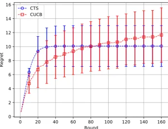
Next, we study the conjunctive analogue of the problem that we consider, where the goal of the search engine is to maximize the number of users with lists that do not contain unattractive pages, and when examining their lists, users provide feedback by reporting the first unattractive page. Formally,
pS(i,j)= 8 > < > : 1 if j = S(i, 1) Qk 1 k0=1pi,S(i,k0) if9k 6= 1 : j = S(i, k) 0 otherwise
and r(S, ppp) =PLi=1QKk=1pi,S(i,k). In this setting, we
let L = 1, R = 1000000, K = 999999, and set all pi,j=
1 except for one, which is set to 1/3. Essentially, we are trying to find the one page that does not certainly attract the user. We run both CTS and CUCB for 160 rounds, and report their regrets averaged over 1000 runs in Figure 2, where error bars represent the standard deviation of the regret. It is observed that CUCB outperforms CTS in the first 80 rounds and CTS outperforms CUCB after the first 80 rounds. This case is specifically constructed to show that CTS does not always uniformly outperform CUCB when there are many good arms but a single bad arm. For CTS to act optimally in this case, the sample from the
Figure 2: Regrets of CTS and CUCB for the conjunc-tive cascading bandit problem.
posterior of the bad arm should be less than the samples from the posteriors of the other arms, which happens with a small probability at the beginning. CUCB is good at the beginning because of the “deterministic” indices. Whenever the bad arm is observed, with high probability its UCB falls below the UCBs of the good arms, and hence, the bad arm is “forgotten” for some time, which leads to better initial performance.
6
CONCLUSION
In this paper we analyzed the regret of CTS for CMAB with PTAs. We proved an order optimal regret bound when the expected reward function is Lipschitz contin-uous without assuming monotonicity of the expected reward function. Our bound includes the 1/p⇤ term
that is unavoidable in general. Future work includes deriving regret bounds under more strict assumptions on the expected reward function such as the triggering probability modulated bounded smoothness condition given in [14] to get rid of the 1/p⇤ term. This is
espe-cially challenging due to the fact that the triggering probabilities depend on the expected arm outcomes, which makes relating the expected rewards under dif-ferent realizations of ✓ (such as given in the proof of Lemma 2) difficult.
Acknowledgment
This work was supported by the Scientific and Techno-logical Research Council of Turkey (TUBITAK) under Grant 215E342.
References
[1] H. Robbins, “Some aspects of the sequential de-sign of experiments,” Bulletin of the American Mathematical Society, vol. 58, no. 5, pp. 527–535, 1952.
[2] T. L. Lai and H. Robbins, “Asymptotically effi-cient adaptive allocation rules,” Advances in Ap-plied Mathematics, vol. 6, no. 1, pp. 4–22, 1985. [3] W. R. Thompson, “On the likelihood that one
unknown probability exceeds another in view of the evidence of two samples,” Biometrika, vol. 25, no. 3/4, pp. 285–294, 1933.
[4] S. Agrawal and N. Goyal, “Analysis of Thompson sampling for the multi-armed bandit problem,” in Proc. 25th Annual Conference on Learning Theory, pp. 39.1–39.26, 2012.
[5] D. Russo and B. Van Roy, “Learning to optimize via posterior sampling,” Mathematics of Opera-tions Research, vol. 39, no. 4, pp. 1221–1243, 2014. [6] R. Agrawal, “Sample mean based index policies with O(log n) regret for the multi-armed bandit problem,” Advances in Applied Probability, vol. 27, no. 4, pp. 1054–1078, 1995.
[7] P. Auer, N. Cesa-Bianchi, and P. Fischer, “Finite-time analysis of the multiarmed bandit problem,” Machine Learning, vol. 47, pp. 235–256, 2002. [8] Y. Gai, B. Krishnamachari, and R. Jain,
“Combi-natorial network optimization with unknown vari-ables: Multi-armed bandits with linear rewards and individual observations,” IEEE/ACM Trans-actions on Networking, vol. 20, no. 5, pp. 1466– 1478, 2012.
[9] B. Kveton, Z. Wen, A. Ashkan, and C. Szepesvari, “Tight regret bounds for stochastic combinatorial
semi-bandits,” in Proc. 18th International Con-ference on Artificial Intelligence and Statistics, pp. 535–543, 2015.
[10] W. Chen, Y. Wang, and Y. Yuan, “Combinatorial multi-armed bandit: General framework and appli-cations,” in Proc. 30th International Conference on Machine Learning, pp. 151–159, 2013.
[11] G. L. Nemhauser, L. A. Wolsey, and M. L. Fisher, “An analysis of approximations for maximizing sub-modular set functions–I,” Mathematical Program-ming, vol. 14, no. 1, pp. 265–294, 1978.
[12] S. Wang and W. Chen, “Thompson sampling for combinatorial semi-bandits,” in Proc. 35th International Conference on Machine Learning, pp. 5114–5122, 2018.
[13] W. Chen, Y. Wang, Y. Yuan, and Q. Wang, “Com-binatorial multi-armed bandit and its extension to probabilistically triggered arms,” The Jour-nal of Machine Learning Research, vol. 17, no. 1, pp. 1746–1778, 2016.
[14] Q. Wang and W. Chen, “Improving regret bounds for combinatorial semi-bandits with probabilisti-cally triggered arms and its applications,” in Proc. Advances in Neural Information Processing Sys-tems, pp. 1161–1171, 2017.
[15] A. O. Saritac and C. Tekin, “Combinatorial multi-armed bandit with probabilistically triggered arms: A case with bounded regret,” arXiv preprint arXiv:1707.07443, 2017.
[16] B. Kveton, Z. Wen, A. Ashkan, H. Eydgahi, and B. Eriksson, “Matroid bandits: Fast combinatorial optimization with learning,” in Proc. 30th Con-ference on Uncertainty in Artificial Intelligence, pp. 420–429, 2014.
[17] A. Gopalan, S. Mannor, and Y. Mansour, “Thomp-son sampling for complex online problems,” in Proc. 31st International Conference on Machine Learning, pp. 100–108, 2014.
[18] Z. Wen, B. Kveton, and A. Ashkan, “Efficient learning in large-scale combinatorial semi-bandits,” in Proc. 32nd International Conference on Ma-chine Learning, pp. 1113–1122, 2015.
[19] D. Kempe, J. Kleinberg, and E. Tardos, “Max-imizing the spread of influence through a social network,” in Proc. 9th ACM SIGKDD Interna-tional Conference on Knowledge Discovery and Data Mining, pp. 137–146, 2003.
[20] B. Kveton, C. Szepesvari, Z. Wen, and A. Ashkan, “Cascading bandits: Learning to rank in the cas-cade model,” in Proc. 32nd International Confer-ence on Machine Learning, pp. 767–776, 2015. [21] M. Mitzenmacher and E. Upfal, Probability and
computing: Randomized algorithms and probabilis-tic analysis. Cambridge University Press, 2005.