CERN-EP-2019-018 2020/05/23
CMS-TOP-17-020
Search for new physics in top quark production in dilepton
final states in proton-proton collisions at
√
s = 13 TeV
The CMS Collaboration
∗Abstract
A search for new physics in top quark production is performed in proton-proton col-lisions at 13 TeV. The data set corresponds to an integrated luminosity of 35.9 fb−1 collected in 2016 with the CMS detector. Events with two opposite-sign isolated lep-tons (electrons or muons), and b quark jets in the final state are selected. The search is sensitive to new physics in top quark pair production and in single top quark pro-duction in association with a W boson. No significant deviation from the standard model expectation is observed. Results are interpreted in the framework of effective field theory and constraints on the relevant effective couplings are set, one at a time, using a dedicated multivariate analysis. This analysis differs from previous searches for new physics in the top quark sector by explicitly separating tW from tt events and exploiting the specific sensitivity of the tW process to new physics.
”Published in the European Physical Journal C as doi:10.1140/epjc/s10052-019-7387-y.”
c
2020 CERN for the benefit of the CMS Collaboration. CC-BY-4.0 license
∗See Appendix A for the list of collaboration members
1
Introduction
Because of its large mass, close to the electroweak (EW) symmetry breaking scale, the top quark is predicted to play an important role in several new physics scenarios. If the new physics scale is in the available energy range of the CERN LHC, the existence of new physics could be di-rectly observed via the production of new particles. Otherwise, new physics could affect stan-dard model (SM) interactions indirectly, through modifications of SM couplings or enhance-ments of rare SM processes. In this case, it is useful to introduce a model independent ap-proach to parametrize and constrain possible deviations from SM predictions, independently of the fundamental theory of new physics.
Several searches for new physics in the top quark sector including new non-SM couplings of the top quark have been performed at the Tevatron and LHC colliders [1–10]. Most of the previous analyses followed the anomalous coupling approach in which the SM Lagrangian is extended for possible new interactions. Another powerful framework to parametrize deviations with respect to the SM prediction is the effective field theory (EFT) [11, 12]. Constraints obtained on anomalous couplings can be translated to the effective coupling bounds [1, 13]. Several groups have performed global fits of top quark EFT to unfolded experimental data from the Teva-tron and LHC colliders [14, 15]. Due to the limited access to data and details of the associated uncertainties, correlations between various cross section measurements and related uncertain-ties are neglected in a global fit on various unfolded measurements. On the other hand, EFT operators could affect backgrounds for some processes constructively or destructively while cross sections are measured with the SM assumptions for background processes. Inside the CMS Collaboration and with direct access to data, all mentioned points could be considered properly.
In this paper, the EFT approach is followed to search for new physics in the top quark sector in the dilepton final states. In Refs. [13, 16], all dimension-six operators that contribute to top quark pair (tt) production and single top quark production in association with a W boson (tW) are investigated. The operators and the related effective Lagrangians, which are relevant for dilepton final states, can be written as [12]:
Oφ(3q)= (φ+τiDµφ)(q γµτiq), Leff = C(φ3q) √ 2Λ2gv 2b γµP LtW−µ +h.c., (1) OtW = (q σµ ν τit)φ˜Wiµ ν, Leff = −2 CtW Λ2 vb σ µ νP Rt∂νW − µ +h.c., (2) OtG = (q σµ ν λat)φ˜Gaµ ν, Leff = CtG √ 2Λ2v(t σ µ ν λat)Gaµ ν+h.c., (3) OG = fabcGaνµ Gbρν G cµ ρ , Leff = CG Λ2 fabcG aν µ G bρ ν G cµ ρ , (4) Ou(c)G = (q σµ νλat)φ˜Gµ νa , Leff = Cu(c)G √ 2Λ2v(u(c)σ µ ν λat)Gaµ ν+h.c., (5) where Dµ =∂µ−igs12λaGµa −ig 1 2τiWiµ−ig 0 YBµ, Wiµ ν =∂µWiν−∂νWiµ+geijkWµjWkν, G a µ ν =
∂µGaν−∂νGaµ+gsfabcGbµGcν, σµ ν = 12[γµ, γν], PL,R = 12(1∓γ5), and the symbols q, t and φ ( ˜φ=eφ∗) in the operators represent the left-handed quark doublet, the right-handed top quark singlet, and the Higgs boson doublet fields, respectively. The parameters C(φ3q), CtW, CtG, CG and Cu(c)Gstand for the dimensionless Wilson coefficients, also called effective couplings. The
variableΛ represents the energy scale beyond which new physics becomes relevant. A detailed description of the operators is given in Refs. [13, 16, 17]. In this analysis, four-fermion operators
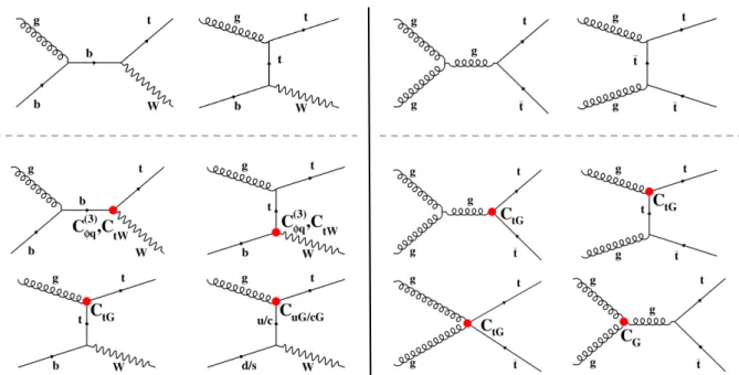
Figure 1: Representative Feynman diagrams for the tW (left panel) and tt (right panel) produc-tion at leading order. The upper row presents the SM diagrams, the middle and lower rows present diagrams corresponding to the O(φ3q), OtW,OtG, OG and Ou/cGcontributions.
involved in tt production are not probed. Up to orderΛ−2, the tW and tt production cross sec-tions and most of the differential observables considered in this analysis do not receive CP-odd contributions. Therefore, we only probe CP-even operators with real coefficients. The opera-tors O(φ3q) and OtW modify the SM interaction between the W boson, top quark, and b quark (Wtb). We consider the EFT effects in the production of top quarks not in their decays [18]. The operator OtG is called the chromomagnetic dipole moment operator of the top quark and can arise from various models of new physics [19, 20]. The triple-gluon field strength operator OG represents the only genuinely gluonic CP conserving term that can appear at dimension six within an effective strong interaction Lagrangian. Although it is shown that jet production at the LHC can set a tight constraint on the CG[21], tt production is also considered as a promising channel [22, 23]. The operators OuG and OcG lead to flavor-changing neutral current (FCNC) interactions of the top quark and contribute to tW production. The effect of introducing new couplings C(φ3q), CtW, CtG and Cu(c)G can be investigated in tW production. The
chromomag-netic dipole moment operator of the top quark also affects tt production. In the case of CG coupling, only tt production is modified. It should be noted that the OtW and OtG operators with imaginary coefficients lead to CP-violating effects. Representative Feynman diagrams for SM and new physics contributions in tW and tt production are shown in Fig. 1.
A variety of limits have been set on the Wtb anomalous coupling through single top quark t-channel production and measurements of the W boson polarization from top quark decay by the D0 [1], ATLAS [2, 3] and CMS [4, 5] Collaborations. Direct limits on the top quark chromomagnetic dipole moment have been obtained by the CMS Collaboration at 7 and 13 TeV using top quark pair production events [6, 10]. Searches for top quark FCNC interactions have been performed at the Tevatron [7, 8] and LHC [4, 9] via single top quark production and limits are set on related anomalous couplings.
In this paper, a search for new physics in top quark production using an EFT framework is reported. This is the first such search for new physics that uses the tW process. Final states
with two opposite-sign isolated leptons (electrons or muons) in association with jets identified as originating from the fragmentation of a bottom quark (“b jets”) are analyzed. The search is sensitive to new physics contributions to tW and tt production, and the six effective couplings, CG, C(φ3q), CtW, CtG, CuG, and CcG, are constrained assuming one non-zero effective coupling at a time. The effective couplings affect both the rate of tt and tW production and the kine-matic distributions of final state particles. For the C(φ3q), CtW, CtG, and CG effective couplings, the deviation from the SM prediction is dominated by the interference term between SM and new physics diagrams, which is linear with respect to the effective coupling. Therefore, the kinematic distributions of the final-state particles vary as a function of the Wilson coefficients. For small effective couplings the kinematic distributions approach those predicted by the SM. On the other hand, the new physics terms due to the CuG and CcG effective couplings do not interfere with the SM tW process, and the kinematic distributions of final-state particles are de-termined by the new physics terms independently of the SM prediction. In this analysis, we use the rates of tW and tt production to probe the C(φ3q), CtW, CtG, and CGeffective couplings. Vari-ations in both rate and kinematic distributions of final-state particles are employed to probe the CuG and CcG effective couplings. The analysis utilizes proton-proton (pp) collision data collected by the CMS experiment in 2016 at a center-of-mass energy of 13 TeV, corresponding to an integrated luminosity of 35.9 fb−1.
The paper is structured as follows. In Section 2, a description of the CMS detector is given and the simulated samples used in the analysis are detailed. The event selection and the SM background estimation are presented in Section 3. Section 4 presents a description of the signal extraction procedure. An overview of the systematic uncertainty treatment is given in Section 5. Finally, the constraints on the effective couplings are presented in Section 6, and a summary is given in Section 7.
2
The CMS detector and event simulation
The central feature of the CMS apparatus is a superconducting solenoid of 6 m internal diame-ter, providing a magnetic field of 3.8 T. Within the solenoid volume are a silicon pixel and strip tracker, a lead tungstate crystal electromagnetic calorimeter (ECAL), and a brass and scintillator hadron calorimeter, each composed of a barrel and two endcap sections. Forward calorimeters extend the pseudorapidity (η) coverage provided by the barrel and endcap detectors. Muons are detected in gas-ionisation chambers embedded in the steel flux-return yoke outside the solenoid. A more detailed description of the CMS detector, together with a definition of the coordinate system used and the relevant kinematic variables, can be found in Ref. [24].
The Monte Carlo (MC) samples for the tt, tW and diboson (VV=WW, WZ, ZZ) SM processes are simulated using the POWHEG-BOXevent generator (v1 for tW, v2 for tt and diboson) [25– 28] at the next-to-leading order (NLO), interfaced withPYTHIA(v8.205) [29] to simulate parton showering and to match soft radiations with the contributions from the matrix elements. The
PYTHIAtune CUETP8M1 [30] is used for all samples except for the tt sample, for which the tune CUETP8M2 [31] is used. The NNPDF3.0 [32] set of the parton distribution functions (PDFs) is used. The tt and tW samples are normalized to the next-to-next-to-leading order (NNLO) and approximate NNLO cross section calculations, respectively [33, 34]. In order to better describe the transverse momentum (pT) distribution of the top quark in tt events, the top quark pT spectrum simulated withPOWHEGis reweighted to match the differential top quark pT distri-bution at NNLO Quantum ChromoDynamics (QCD) accuracy and including EW corrections calculated in Ref. [35]. Other SM background contributions, from Drell–Yan (DY), tt +V, tt +γ,
and W+γprocesses, are simulated at NLO using the MADGRAPH5 aMC@NLO(v2.2.2) event generator [36–38], interfaced with PYTHIA v8 for parton showering and hadronization. The events include the effects of additional pp interactions in the same or nearby bunch crossings (pileup) and are weighted according to the observed pileup distribution in the analyzed data. The CMS detector response is simulated using GEANT4 (v9.4) [39, 40], followed by a detailed trigger simulation. Simulated events are reconstructed with the same algorithms as used for data.
In order to calculate the total cross sections for the tt and tW processes and generate events in the presence of new effective interactions, the operators of Eqs. 1–5 have been implemented in the universal FEYNRULESoutput (UFO) format [41] through the FEYNRULESpackage [42]. The
output EFT model is used in the MADGRAPH5 aMC@NLO(v2.2.2) event generator [36, 37]. If
we allow for the presence of one operator at a time, the total cross section up toO(Λ−4)can be
parametrized as
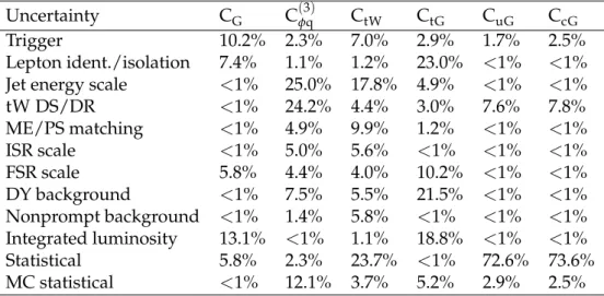
σ=σSM+Ciσi(1)+C2iσi(2), (6) where the Cis are effective couplings introduced in Eqs. 1–5. Here, σi(1) is the contribution to the cross section due to the interference term between the SM diagrams and diagrams with one EFT vertex. The cross section σi(2)is the pure new physics contribution. We use the most precise available SM cross section prediction, which are σSMtt =832+−2029(scales)±35(PDF+αS)pb and σSMtW = 71.7±1.8 (scales)±3.4(PDF+αS)pb for tt and tW production, respectively [33, 34], where the αSis strong coupling constant. The first uncertainty reflects the uncertainties in the factorization and renormalization scales. In the framework of EFT, the σi(1)and σi(2)terms have been calculated at NLO accuracy for all of the operators, except OG [16, 43, 44]. At the time the work for this paper was concluded, there was no available UFO model including the OG operator at the NLO. The values of σi(1) and σi(2) for various effective couplings at LO and available K factors are given in Table 1.
Table 1: Contribution to the cross section due to the interference between the SM diagrams and diagrams with one EFT vertex (σi(1)), and the pure new physics (σi(2)) for tt and tW production [in pb ] for the various effective couplings forΛ = 1 TeV. The respective K factors (σiNLO/σiLO) are also shown.
Channel Contribution CG Cφ(3q) CtW CtG CuG CcG tt σi(1)−LO 31.9 pb — — 137 pb — — K(1) — — — 1.48 — — σi(2)−LO 102.3 pb — — 16.4 pb — — K(2) — — — 1.44 — — t W σi(1)−LO — 6.7 pb −4.5 pb 3.3 pb 0 0 K(1) — 1.32 1.27 1.27 0 0 σi(2)−LO — 0.2 pb 1 pb 1.2 pb 16.2 pb 4.6 pb K(2) — 1.31 1.18 1.06 1.27 1.27
3
Event selection and background estimation
The event selection for this analysis is similar to the one used in Ref. [10]. The events of interest are recorded by the CMS detector using a combination of dilepton and single-lepton triggers.
Single-lepton triggers require at least one isolated electron (muon) with pT >27(24)GeV. The dilepton triggers select events with at least two leptons with loose isolation requirements and pTfor the leading and sub-leading leptons greater than 23 and 12 (17 and 8) GeV for the ee (µµ) final state. In the eµ final state, in the case of the leading lepton being an electron, the events are triggered if the electron-muon pair has a pT greater than 23 and 8 GeV for the electron and muon, respectively. In the case of the leading lepton being a muon, the trigger thresholds are 23 and 12 GeV for the muon and electron, respectively [45].
Offline, the particle-flow (PF) algorithm [46] aims to reconstruct and identify each individual particle with an optimized combination of information from the various elements of the CMS detector. Electron candidates are reconstructed using tracking and ECAL information [47]. Re-quirements on electron identification variables based on shower shape and track-cluster match-ing are further applied to the reconstructed electron candidates, together with isolation crite-ria [10, 47]. Electron candidates are selected with pT > 20 GeV and |η| < 2.4. Electron candi-dates within the range 1.444< |η| <1.566, which corresponds to the transition region between the barrel and endcap regions of the ECAL, are not considered. Information from the tracker and the muon spectrometer are combined in a global fit to reconstruct muon candidates [48]. Muon candidates are further required to have a high-quality fit including a minimum number of hits in both systems, and to be isolated [10, 48]. The muons used in this analysis are selected inside the fiducial region of the muon spectrometer,|η| <2.4, with a minimum pTof 20 GeV. The PF candidates are clustered into jets using the anti-kT algorithm with a distance parame-ter of 0.4 [49–51]. Jets are calibrated in data and simulation, accounting for energy deposits of particles from pileup [52]. Jets with pT > 30 GeV and|η| < 2.4 are selected; loose jets are de-fined as jets with the pTrange between 20 and 30 GeV. Jets originating from the hadronization of b quarks are identified using the combined secondary vertex algorithm [53]; this algorithm combines information from track impact parameters and secondary vertices identified within a given jet. The chosen working point provides a signal identification efficiency of approximately 68% with a probability to misidentify light-flavor jets as b jets of approximately 1% [53]. The missing transverse momentum vector~pmiss
T is defined as the projection on the plane
perpendic-ular to the proton beams axis of the negative vector sum of the momenta of all reconstructed PF candidates in the event [54]. Corrections to the jet energies are propagated to~pTmiss. Its magnitude is referred to as pmissT .
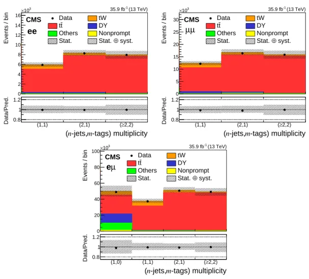
Events are required to have at least two leptons (electrons or muons) with opposite sign and with an invariant mass above 20 GeV. The leading lepton must fulfill pT > 25 GeV. For the same-flavor lepton channels, to suppress the DY background, the dilepton invariant mass must not be within 15 GeV of the Z boson mass and a minimal value (of 60 GeV) on pmissT is applied. The events are divided into the ee, eµ, and µµ channels according to the flavors of the two lep-tons with the highest pTand are further categorized in different bins depending on the number of jets (“n-jets”) and number b-tagged jets (“m-tags”) in the final state. The largest number of tW events is expected in the category with exactly one b-tagged jet (1-jet,1-tag) followed by the category with two jets, of which one a b jet (2-jets,1-tag). Events in the categories with more than two jets and exactly two b-tagged jets are dominated by the tt process (≥2-jets,2-tags). Categories with zero b jets are dominated by DY events in the ee and µµ channels and are not used in the analysis. However, in the eµ channel, the contamination of DY events is lower and a significant number of tW events is present in the category with one jet and zero b-tagged jets (1-jet,0-tag). The latter category is included in this analysis. In Fig. 2, the data in the ten search regions are shown together with the SM background predictions.
Events / bin 0 2 4 6 8 10 12 14 16 3 10 × Data tW t t DY Others Nonprompt Stat. Stat. ⊕ syst.
CMS (13 TeV) -1 35.9 fb ee -tags) multiplicity m -jets, n ( (1,1) (2,1) (≥2,2) Data/Pred. 0.8 1 1.2 Events / bin 0 5 10 15 20 25 30 3 10 × Data tW t t DY Others Nonprompt Stat. Stat. ⊕ syst.
CMS (13 TeV) -1 35.9 fb µ µ -tags) multiplicity m -jets, n ( (1,1) (2,1) (≥2,2) Data/Pred. 0.8 1 1.2 Events / bin 0 20 40 60 80 100 3 10 × Data tW t t DY Others Nonprompt Stat. Stat. ⊕ syst.
CMS (13 TeV) -1 35.9 fb µ e -tags) multiplicity m -jets, n ( (1,0) (1,1) (2,1) (≥2,2) Data/Pred. 0.8 1 1.2
Figure 2: The observed number of events and SM background predictions in the search regions of the analysis for the ee (upper left), µµ (upper right), and eµ (lower) channels. The hatched bands correspond to the quadratic sum of statistical and systematic uncertainties in the event yield for the SM background predictions. The ratios of data to the sum of the predicted yields are shown at the bottom of each plot. The narrow hatched bands represent the contribution from the statistical uncertainty in the MC simulation.
from simulated samples and are normalised to the integrated luminosity of the data. These contributions originate mainly from tt, tW and DY production. Other SM processes, such as diboson, tt +V and tt +γ have significantly smaller contributions.
To correct the DY simulation for the efficiency of the pmissT threshold and for the mismodel-ing of the heavy-flavour content, scale factors are derived usmismodel-ing the ratio of the numbers of simulated events inside and outside the dilepton invariant mass window, 76 to 106 GeV. The observed event yield inside the window is scaled to estimate the DY background outside the mass window [55].
The nonprompt lepton backgrounds which contain fake lepton(s) from a misreconstructed γ or jet(s) are also considered. The contribution of misidentified or converted γ events from the Wγ process is estimated from MC simulation. The contribution from W+jets and multijet processes is estimated by a data-based technique using events with same-sign leptons. The method is based on the assumption that the probability of assigning positive or negative charge to the fake lepton is equal. Therefore, the background contribution from fake leptons in the final selection (opposite-sign sample) can be estimated from the corresponding sample with
same-sign leptons. In this latter same-same-sign event sample, the remaining small contribution from prompt-lepton backgrounds is subtracted from data using MC samples.
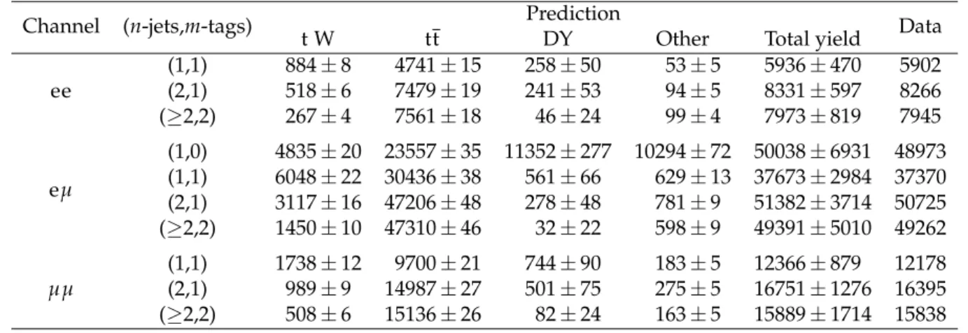
After all selections, the expected numbers of events from tW, tt, DY, and remaining back-ground contributions mentioned above, as well as the total number of backback-ground events are reported in Table 2 for the ee, eµ, and µµ channels and for the various (n-jets,m-tags) categories. We find generally very good agreement between data and predictions, within the uncertainties of the data.
Table 2: Number of expected events from tW, tt and DY production, from the remaining back-grounds (other), total background contribution and observed events in data after all selections for the ee, eµ, and µµ channels and for different (n-jets,m-tags) categories. The uncertainties correspond to the statistical contribution only for the individual background predictions and to the quadratic sum of the statistical and systematic contributions for the total background predictions.
Channel (n-jets,m-tags) Prediction Data
t W tt DY Other Total yield
ee (1,1) 884±8 4741±15 258±50 53±5 5936±470 5902 (2,1) 518±6 7479±19 241±53 94±5 8331±597 8266 (≥2,2) 267±4 7561±18 46±24 99±4 7973±819 7945 eµ (1,0) 4835±20 23557±35 11352±277 10294±72 50038±6931 48973 (1,1) 6048±22 30436±38 561±66 629±13 37673±2984 37370 (2,1) 3117±16 47206±48 278±48 781±9 51382±3714 50725 (≥2,2) 1450±10 47310±46 32±22 598±9 49391±5010 49262 µµ (1,1) 1738±12 9700±21 744±90 183±5 12366±879 12178 (2,1) 989±9 14987±27 501±75 275±5 16751±1276 16395 (≥2,2) 508±6 15136±26 82±24 163±5 15889±1714 15838
4
Signal extraction using neural networks tools
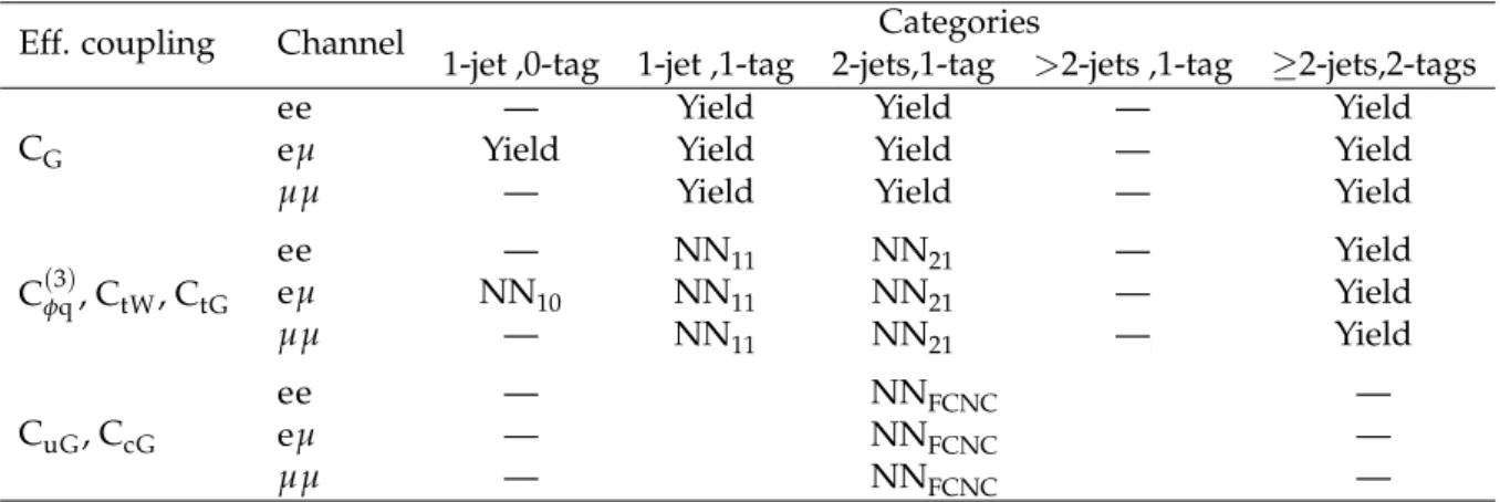
The purpose of the analysis is to search for deviations from the SM predictions in the tW and tt production due to new physics, parametrized with the presence of new effective couplings. In order to investigate the effect of the non-zero effective couplings, it is important to find suitable variables with high discrimination power between the signal and the background. Depending on the couplings, the total yield or the distribution of the output of a neural network (NN) algorithm is employed, as summarized in Table 3. The NN algorithm used in this analysis is a multilayer perceptron [56].
All the effective couplings introduced in Section 1 can contribute to tW production except the triple gluon field strength operator, OG which only affects tt production. As observed in pre-vious analysis [22] and confirmed here, the top quark pT distribution is sensitive to the triple-gluon field-strength operator. The kinematic distributions of final-state particles show less dis-crimination power than the top quark pTdistribution. In addition, they vary with the value of CG and approach the SM prediction for decreasing values of CG. Therefore, we use the total yield in various categories to constrain the CG effective coupling.
The deviation from the SM tW production because of the interference between the SM and the OtG, O(φ3q), and OtW operators is of the order of 1/Λ2. It is assumed that the new physics scaleΛ is larger than the scale we probe. Therefore, 1/Λ4contributions from the new physics terms are small compared to the contribution from the interference term. The operator O(φ3q) is
Table 3: Summary of the observables used to probe the effective couplings in various (n-jets,m-tags) categories in the ee, eµ, and µµ channels.
Eff. coupling Channel Categories
1-jet ,0-tag 1-jet ,1-tag 2-jets,1-tag >2-jets ,1-tag ≥2-jets,2-tags CG
ee — Yield Yield — Yield
eµ Yield Yield Yield — Yield
µµ — Yield Yield — Yield
C(3)φq, CtW, CtG ee — NN11 NN21 — Yield eµ NN10 NN11 NN21 — Yield µµ — NN11 NN21 — Yield CuG, CcG ee — NNFCNC — eµ — NNFCNC — µµ — NNFCNC —
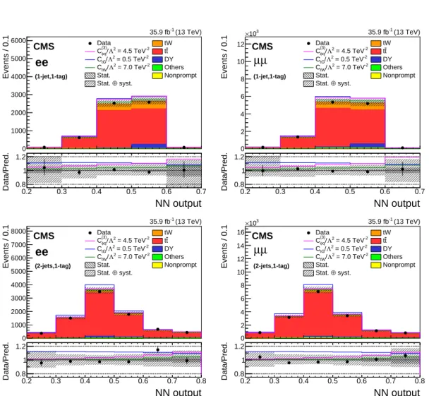
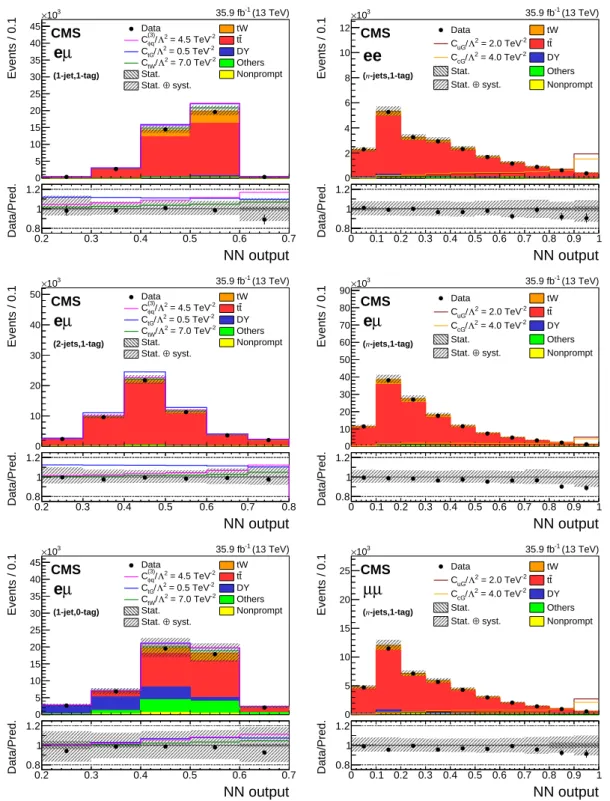
similar to the SM Wtb operator and leads to a rescaling of the SM Wtb vertex [13]. The OtW and OtGoperators lead to the right-handed Wtb interaction and a tensor-like ttg interaction, re-spectively, which are absent in the SM at the first order. Their effects have been investigated via the various kinematic distributions of the final-state particles considered in this analysis and are found to be not distinguishable from the SM tW and tt processes for unconstrained values of the effective couplings within the current precision on data. After the selection described in Section 3, the dominant background comes from tt production, with a contribution of about 90%. In order to observe deviations from SM tW production in the presence of the O(φ3q), OtW, and OtGeffective operators, we need to separate tW events from the large number of tt events. Two independent NNs are trained to separate tt events (the background) and tW events (con-sidered as the signal) in the (1-jet,1-tag) (NN11) and (2-jets,1-tag) (NN21) categories, which have significant signal contributions [57]. For the eµ channel, another NN is used for the (1-jet,0-tag) (NN10) category, in which the tt, WW, and DY events are combined and are considered as the background. A comparison between the observed data and the SM background prediction of the NN output shape in various (n-jets,m-tags) categories is shown for the ee and µµ channels in Fig. 3 and for the eµ channel in Fig. 4 (left column).
The presence of the OuG and OcG operators changes the initial-state particle (see Fig. 1), and leads to different kinematic distributions for the final-state particles, compared to the SM tW process. For these FCNC operators, new physics effects on final-state particle distributions are expected to be distinguishable from SM processes. In order to search for new physics due to the OuG and OcGeffective operators, an NN (NNFCNC) is used to separate SM backgrounds (tt and tW events together) and new physics signals for events with exactly one b-tagged jet with no requirement on the number of light-flavor jets (n-jets,1-tag). The comparison of the NN output for data, SM background and signal (tW events via FCNC interactions) is shown in Fig. 4 (right column) for the ee, eµ, and µµ channels.
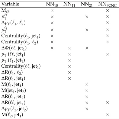
The various input variables for training the NN introduced above are described below and are shown in Table 4.
• M``(where`= e or µ), invariant mass of dilepton system;
• p``T, pTof dilepton system;
• ∆pT(`1,`2), pleading leptonT −psub-leading leptonT ; • p`1
T, pTof leading lepton;
Events / 0.1 0 1000 2000 3000 4000 5000 6000 Data tW -2 = 4.5 TeV 2 Λ / (3) q φ C tt -2 = 0.5 TeV 2 Λ / tG C DY -2 = 7.0 TeV 2 Λ / tW C Others Stat. Nonprompt syst. ⊕ Stat. CMS (13 TeV) -1 35.9 fb ee (1-jet,1-tag) NN output 0.2 0.3 0.4 0.5 0.6 0.7 Data/Pred. 0.8 1 1.2 Events / 0.1 0 2 4 6 8 10 12 3 10 × Data tW -2 = 4.5 TeV 2 Λ / (3) q φ C tt -2 = 0.5 TeV 2 Λ / tG C DY -2 = 7.0 TeV 2 Λ / tW C Others Stat. Nonprompt syst. ⊕ Stat. CMS (13 TeV) -1 35.9 fb µ µ (1-jet,1-tag) NN output 0.2 0.3 0.4 0.5 0.6 0.7 Data/Pred. 0.8 1 1.2 Events / 0.1 0 1000 2000 3000 4000 5000 6000 7000 8000 Data tW -2 = 4.5 TeV 2 Λ / (3) q φ C tt -2 = 0.5 TeV 2 Λ / tG C DY -2 = 7.0 TeV 2 Λ / tW C Others Stat. Nonprompt syst. ⊕ Stat. CMS (13 TeV) -1 35.9 fb ee (2-jets,1-tag) NN output 0.2 0.3 0.4 0.5 0.6 0.7 0.8 Data/Pred. 0.8 1 1.2 Events / 0.1 0 2 4 6 8 10 12 14 16 3 10 × Data tW -2 = 4.5 TeV 2 Λ / (3) q φ C tt -2 = 0.5 TeV 2 Λ / tG C DY -2 = 7.0 TeV 2 Λ / tW C Others Stat. Nonprompt syst. ⊕ Stat. CMS (13 TeV) -1 35.9 fb µ µ (2-jets,1-tag) NN output 0.2 0.3 0.4 0.5 0.6 0.7 0.8 Data/Pred. 0.8 1 1.2
Figure 3: The NN output distributions for data and simulation for the ee (left) and µµ (right) channels in 1-jet, 1-tag (upper) and 2-jets, 1-tag (lower) categories. The hatched bands corre-spond to the quadratic sum of the statistical and systematic uncertainties in the event yield for the sum of signal and background predictions. The ratios of data to the sum of the pre-dicted yields are shown at the lower panel of each graph. The narrow hatched bands represent the contribution from the statistical uncertainty in the MC simulation. In each plot, the ex-pected distributions assuming specific values for the effective couplings (given in the legend) are shown as the solid curves.
Events / 0.1 0 5 10 15 20 25 30 35 40 45 3 10 × Data tW -2 = 4.5 TeV 2 Λ / (3) q φ C tt -2 = 0.5 TeV 2 Λ / tG C DY -2 = 7.0 TeV 2 Λ / tW C Others Stat. Nonprompt syst. ⊕ Stat. CMS (13 TeV) -1 35.9 fb µ e (1-jet,1-tag) NN output 0.2 0.3 0.4 0.5 0.6 0.7 Data/Pred. 0.8 1 1.2 Events / 0.1 0 2 4 6 8 10 12 3 10 × Data tW -2 = 2.0 TeV 2 Λ / uG C tt -2 = 4.0 TeV 2 Λ / cG C DY Stat. Others syst. ⊕ Stat. Nonprompt CMS (13 TeV) -1 35.9 fb ee -jets,1-tag) n ( NN output 0 0.1 0.2 0.3 0.4 0.5 0.6 0.7 0.8 0.9 1 Data/Pred. 0.8 1 1.2 Events / 0.1 0 10 20 30 40 50 3 10 × Data tW -2 = 4.5 TeV 2 Λ / (3) q φ C tt -2 = 0.5 TeV 2 Λ / tG C DY -2 = 7.0 TeV 2 Λ / tW C Others Stat. Nonprompt syst. ⊕ Stat. CMS (13 TeV) -1 35.9 fb µ e (2-jets,1-tag) NN output 0.2 0.3 0.4 0.5 0.6 0.7 0.8 Data/Pred. 0.8 1 1.2 Events / 0.1 0 10 20 30 40 50 60 70 80 90 3 10 × Data tW -2 = 2.0 TeV 2 Λ / uG C tt -2 = 4.0 TeV 2 Λ / cG C DY Stat. Others syst. ⊕ Stat. Nonprompt CMS (13 TeV) -1 35.9 fb µ e -jets,1-tag) n ( NN output 0 0.1 0.2 0.3 0.4 0.5 0.6 0.7 0.8 0.9 1 Data/Pred. 0.8 1 1.2 Events / 0.1 0 5 10 15 20 25 30 35 40 45 3 10 × Data tW -2 = 4.5 TeV 2 Λ / (3) q φ C tt -2 = 0.5 TeV 2 Λ / tG C DY -2 = 7.0 TeV 2 Λ / tW C Others Stat. Nonprompt syst. ⊕ Stat. CMS (13 TeV) -1 35.9 fb µ e (1-jet,0-tag) NN output 0.2 0.3 0.4 0.5 0.6 0.7 Data/Pred. 0.8 1 1.2 Events / 0.1 0 5 10 15 20 25 3 10 × Data tW -2 = 2.0 TeV 2 Λ / uG C tt -2 = 4.0 TeV 2 Λ / cG C DY Stat. Others syst. ⊕ Stat. Nonprompt CMS (13 TeV) -1 35.9 fb µ µ -jets,1-tag) n ( NN output 0 0.1 0.2 0.3 0.4 0.5 0.6 0.7 0.8 0.9 1 Data/Pred. 0.8 1 1.2
Figure 4: The NN output distributions for (left) data and simulation for the eµ channel in 1-jet, 1-tag (upper) and 2-jets, 1-tag (middle) and 1-jet, 0-tag (lower) categories; and for (right) data, simulation, and FCNC signals in the n-jets, 1-tag category used in the limit setting for the ee (upper), eµ (middle), and µµ (lower) channels. The hatched bands correspond to the quadratic sum of the statistical and systematic uncertainties in the event yield for the sum of signal and background predictions. The ratios of data to the sum of the predicted yields are shown at the the lower panel of each graph. The narrow hatched bands represent the contribution from the statistical uncertainty in the MC simulation. In each plot, the expected distributions assuming specific values for the effective couplings (given in the legend) are shown as the solid curves.
energy of selected leptons and jets;
• Centrality(`1, `2), scalar sum of pTof the leading and sub-leading leptons, over total energy of selected leptons and jets;
• ∆Φ(``, jet1),∆Φ between dilepton system and leading jet where Φ is azimuthal an-gle;
• pT(``, jet1), pT of dilepton and leading jet system; • pT(`1, jet1), pTof leading lepton and leading jet system;
• Centrality(``, jet1), scalar sum of pTof the dilepton system and leading jet, over total energy of selected leptons and jets;
• ∆R(`1, `2), √ (η`1−η`2)2 + (Φ`1−Φ`2)2; • ∆R(`1, jet1), √ (η`1 −ηjet1)2 + (Φ`1−Φjet1)2;
• M(`1, jet1), invariant mass of leading lepton and leading jet; • M(jet1, jet2), invariant mass of leading jet and sub-leading jet; • ∆R(`1, jet2), √ (η`1 −ηjet2)2 + (Φ`1−Φjet2)2; • ∆R(``, jet1), √ (η``−ηjet1)2 + (Φ``−Φjet1)2; • ∆pT(`2, jet2), p`2 T −p jet2 T ;
• M(`2, jet1), invariant mass of sub-leading lepton and leading jet.
Table 4: Input variables for the NN used in the analysis in various bins of n-jets and m-tags. The symbols ”×” indicate the input variables used in the four NNs.
Variable NN10 NN11 NN21 NNFCNC M`` × × p``T × × × ∆pT(`1,`2) × × p`1 T × × × Centrality(`1, jet1) × × Centrality(`1, `2) × × ∆Φ(``, jet1) × × × pT(``, jet1) × × pT(`1, jet1) × Centrality(``, jet1) × ∆R(`1, `2) × ∆R(`1, jet1) × M(`1, jet1) × M(jet1, jet2) × ∆R(`1, jet2) × ∆R(``, jet1) × × ∆pT(`2, jet2) × M(`2, jet1) ×
5
Systematic uncertainties
The normalization and shape of the signal and the backgrounds are both affected by different sources of systematic uncertainty. For each source, an induced variation can be parametrized, and treated as a nuisance parameter in the fit that is described in the next section.
A systematic uncertainty of 2.5% is assigned to the integrated luminosity and is used for signal and background rates [58]. The efficiency corrections for trigger and offline selection of leptons were estimated by comparing the efficiency measured in data and in MC simulation using Z → ``events, based on a “tag-and-probe” method as in Ref. [59]. The scale factors obtained are varied by one standard deviation to take into account the corresponding uncertainties in the efficiency. The jet energy scale and resolution uncertainties depend on pTand η of the jet and are computed by shifting the energy of each jet and propagating the variation to ~pTmiss coherently [60].
The uncertainty in the b tagging is estimated by varying the b tagging scale factors within one standard deviation [53]. Effects of the uncertainty in the distribution of the number of pileup interactions are evaluated by varying the effective inelastic pp cross section used to predict the number of pileup interactions in MC simulation by±4.6% of its nominal value [61].
The uncertainty in the DY contribution in categories with one or two b-tagged jets is considered to be 50 and 30% in the eµ and same-flavor dilepton channels, respectively [10, 57]. For the DY normalization in the (1-jet,0-tag) category, an uncertainty of 15% is assigned [62]. In addition, systematic uncertainties related to the PDF, and to the renormalization and factorization scale uncertainty are taken into account for DY process in the (1-jet,0-tag) category. The uncertainty in the yield of nonprompt lepton backgrounds is considered to be 50% [57]. Contributions to the background from tt production in association with a boson, as well as diboson production, are estimated from simulation and a systematic uncertainty of 50% is conservatively assigned [63].
Various uncertainties originate from the theoretical predictions. The effect of the renormal-ization and factorrenormal-ization scale uncertainty from the tt and tW MC generators is estimated by varying the scales used during the generation of the simulation sample independently by a fac-tor 0.5, 1 or 2. Unphysical cases, where one scale fluctuates up while the other fluctuates down, are not considered. The top quark pTreweighting procedure, discussed in Sec. 2, is applied on top of the nominalPOWHEGprediction at NLO to account for the higher-order corrections. The uncertainty in the PDFs for each simulated signal process is obtained using the replicas of the NNPDF 3.0 set [64]. The most recent measurement of the top quark mass by CMS yields a total uncertainty of±0.49 GeV [65]. We consider variations of the top quark mass due to this uncertainty and they are found to be insignificant. At NLO QCD, tW production is expected to interfere with tt production [66]. Two schemes for defining the tW signal in a way that distin-guishes it from the tt production have been compared in the analysis: the “diagram removal” (DR), in which all doubly resonant NLO tW diagrams are removed, and the “diagram sub-traction” (DS), where a gauge-invariant subtractive term modifies the NLO tW cross section to locally cancel the contribution from tt production [66–68]. The DR method is used for the nom-inal tW sample and the difference with respect to the sample simulated using the DS method is taken as a systematic uncertainty. The model parameter hdampin ttPOWHEG [25] that controls the matching of the matrix elements to thePYTHIAparton showers is varied from a top quark
mass default value of 172.5 GeV by factors of 0.5 and 2 for estimating the uncertainties from the matching between jets from matrix element calculations and parton shower emissions. The renormalization scale for QCD emissions in the initial- and final-state radiation (ISR and FSR) is varied up and down by factors of 2 and√2, respectively, to account for parton shower QCD scale variation error in both tt and tW samples [69]. In addition, several dedicated tt sam-ples are used to estimate shower modeling uncertainties in both underlying event and color re-connections [10, 31, 69]. To estimate model uncertainties, tW and tt samples are generated withPOWHEGas described in Sec. 2, varying the relevant model parameters with respect to the
nominal samples.
6
Constraints on the effective couplings
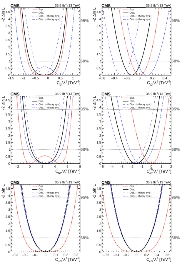
The six Wilson coefficients sensitive to new physics contributions in top quark interactions, as defined in Eqs. 1–5, are tested separately in the observed data. The event yields and the NN output distributions in each analysis category, summarized in Table 3, are used to construct a binned likelihood function. All sources of systematic uncertainty, described in Section 5, are taken into account as nuisance parameters in the fit. A simultaneous binned maximum-likelihood fit is performed to find the best fit value for each Wilson coefficient together with 68 and 95% confidence intervals (CIs) [70]. In this Section, distributions of the log-likelihood functions are shown with one nonzero effective coupling at a time forΛ = 1 TeV.
The SM cross section prediction for the tt and tW processes, σi(1) and σi(2) (see Table 1), are accompanied by uncertainties in scales and PDFs. These theoretical uncertainties can affect the bounds on the Wilson coefficients. In order to study this effect, the fit is performed on data, while theoretical uncertainties are varied within one standard deviation and are shown together with the nominal results in the likelihood scan plots in Fig. 5. The nominal theoretical cross sections for tt and tW processes are varied by [+4.8%,−5.5%] and [+5.4%,−5.4%] , respec-tively. These variations cover the uncertainties arising from the variations of factorization and renormalization scales and PDFs [10, 34]. The scale variations for σi(1)and σi(2)are evaluated to be within 1 to 25%. We assumed that the scale uncertainty is 100% correlated among the terms σSM, σi(1), and σi(2).
6.1 Exclusion limits on the CG effective coupling
In order to constrain the CG coupling, the effect on the tt rate in various (n-jets,m-tags) cat-egories is considered. The impact of the difference between the kinematic distributions of tt events from the OG interaction and from the SM interactions on the acceptance is evaluated to be 3% for CG ∼ 1. This uncertainty is considered only for the CG coupling since the top pT spectrum is affected considerably by this operator, while other operators lead to a pT spec-trum similar to the SM prediction for unconstrained values of the probed Wilson coefficients. The fit is performed simultaneously on the observed event yields in the categories presented in Fig. 2 in the (1-jet,1-tag), (2-jets,1-tag), and (≥2-jets,2-tags) categories for the ee, eµ, and µµ channels. In addition, the (1-jet,0-tag) category is included only for the eµ channel. The main limiting factor on the constraints in the CGcoupling is the uncertainty in the signal acceptance found after maximizing the likelihood, followed by uncertainties in the integrated luminosity calibration and the trigger scale factor.
The results of the fit for the individual channels and for all channels combined are listed in the first row of Table 5.
The results of the likelihood scans of the CG coupling are shown in Fig. 5 (upper left plot). The likelihood scan result of the nominal fit, in which the nominal values of σSM, σi(1), and σi(2) terms are assumed, is shown as the thick curve. The thin dashed curves are the results of the fit to the observed data when the assumed values of the σSM, σi(1), and σi(2) terms are varied due to the scale and PDF uncertainties. As a second-order parametrization, given by Eq. 6 is used to fit the data, the resulting likelihood function could have two minima, as can be seen in some of the plots in Fig. 5.
6.2 Exclusion limits on the CtG, C(φq3), and CtW effective couplings
In order to set limits on the effective couplings CtG, C(φ3q), and CtW, we utilize the NN output distributions for both data and MC expectation in the (1-jet,1-tag) and (2-jets,1-tag) regions and event yields in the (≥2-jets,2-tags) region for the three dilepton channels. The inclusion of the (≥2-jets,2-tags) and (2-jets,1-tag) categories provides a constraint of the normalization and systematic uncertainties in the tt background. In addition, the (1-jet,0-tag) category is included for the eµ channel to increase the signal sensitivity. The results of the likelihood scans of the CtG, C(φ3q), and CtW Wilson coefficients are shown in Fig. 5 for the combination of all channels. The inclusion of the CtG coupling to the tW process tightens the 2 standard deviations band by 7%. The results for the individual channels, and the combined results are listed in Table 5 (second, third, and fourth rows). The three main sources of uncertainty that affect the interval determination are uncertainties in the DY estimation, integrated luminosity, and lepton identification scale factors for CtG; jet energy scale, tt and tW interference at NLO, and statistical uncertainty in MC samples for C(φ3q); statistical uncertainty in data, jet energy scale, and thePOWHEGmatching method for CtWeffective couplings.
6.3 Exclusion limits on the CuG and CcG effective couplings
Since the tW production via FCNC interactions does not interfere with the SM tW process (with the assumption of |Vtd| = |Vts| = 0), the FCNC signal sample is used to set upper bounds on the related Wilson coefficients. Events with exactly one b-tagged jet are included in the limit setting procedure with no requirement on the number of light-flavor jets (n-jets,1-tag). The observed (median expected) 95% confidence level (CL) upper limits on the product of cross section times branching fractions σ(pp → tW)B(W → `ν)2 for the CuG and CcG FCNC signals for the combination of the ee, µµ, and eµ channels are found to be 0.11 (0.20) pb and 0.13 (0.26) pb, respectively. These results are used to calculate upper limits on the Wilson coefficients CuG, CcG, and on the branching fractionsB(t →ug)andB(t →cg). The limits on the CuGand CcG couplings are summarized in the last two rows of Table 5, and correspond to the observed (expected) limits onB(t → ug) <0.12 (0.22)% andB(t →cg) <0.53 (1.05)% at 95% CL. The statistical uncertainty in data is the dominant source of uncertainty affecting the limits on the FCNC couplings. The second and third most important uncertainties originate from tt and tW interferences at NLO and FSR in tt events.
The observed best fit together with one and two standard deviation bounds on the six Wilson coefficients, C(φ3q), CtW, CtG, CG, CuG, and CcG, obtained from the combination of all channels are shown in Fig. 6. Table 6 summarizes the effect of the most important uncertainty sources on the observed allowed intervals.
7
Summary
A search for new physics in top quark interactions is performed using tt and tW events in dilepton final states. The analysis is based on data collected in pp collisions at 13 TeV by the CMS detector in 2016, corresponding to an integrated luminosity of 35.9 fb−1. No significant excess above the standard model background expectation is observed. For the first time, both tt and tW production are used simultaneously in a model independent search for effective couplings. The six effective couplings, CG, CtG, CtW, Cφ(3q), CuG, and CcG are constrained us-ing a dedicated multivariate analysis. The constraints presented, obtained by considerus-ing one operator at a time, are a useful first step toward more global approaches.
] -2 [TeV 2 Λ / G C 1.5 − −1 −0.5 0 0.5 1 ln L ∆ -2 0 0.5 1 1.5 2 2.5 3 3.5 4 4.5 Exp.Obs. theory sys.) + Obs. ( theory sys.) − Obs. ( 68% 95% CMS 35.9 fb-1 (13 TeV) ] -2 [TeV 2 Λ / tG C 0.6 − −0.4 −0.2 0 0.2 0.4 ln L ∆ -2 0 0.5 1 1.5 2 2.5 3 3.5 4 4.5 Exp.Obs. theory sys.) + Obs. ( theory sys.) − Obs. ( 68% 95% CMS 35.9 fb-1 (13 TeV) ] -2 [TeV 2 Λ / tW C 2 − 0 2 4 6 8 ln L ∆ -2 0 0.5 1 1.5 2 2.5 3 3.5 4 4.5 Exp.Obs. theory sys.) + Obs. ( theory sys.) − Obs. ( 68% 95% CMS 35.9 fb-1 (13 TeV) ] -2 [TeV 2 Λ / (3) q φ C 5 − −4 −3 −2 −1 0 1 2 ln L ∆ -2 0 0.5 1 1.5 2 2.5 3 3.5 4 4.5 Exp.Obs. theory sys.) + Obs. ( theory sys.) − Obs. ( 68% 95% CMS 35.9 fb-1 (13 TeV) ] -2 [TeV 2 Λ / uG C 0.3 − −0.2 −0.1 0 0.1 0.2 0.3 ln L ∆ -2 0 0.5 1 1.5 2 2.5 3 3.5 4 4.5 Exp.Obs. theory sys.) + Obs. ( theory sys.) − Obs. ( 68% 95% CMS 35.9 fb-1 (13 TeV) ] -2 [TeV 2 Λ / cG C 0.6 − −0.4 −0.2 0 0.2 0.4 0.6 ln L ∆ -2 0 0.5 1 1.5 2 2.5 3 3.5 4 4.5 Exp.Obs. theory sys.) + Obs. ( theory sys.) − Obs. ( 68% 95% CMS 35.9 fb-1 (13 TeV)
Figure 5: Observed (solid) and expected (dotted) log likelihoods for the effective couplings: CG (upper left), CtG(upper right), CtW (middle left), Cφq (middle right), CuG (lower left), and CcG (lower right). The dashed curves represent fits to the observed data with the variations of normalization due to the theoretical uncertainties.
Table 5: Summary of the observed and expected allowed intervals on the effective couplings obtained in the ee, eµ, and µµ channels, and all channels combined. All sources of systematic uncertainty, described in Section 5, are taken into account with the exception of the uncertain-ties on the SM cross section predictions for the tt and tW processes.
Effective
Channel Observed [TeV
−2] Expected [TeV−2]
coupling Best fit [68% CI] [95% CI] Best fit [68% CI] [95% CI] CG/Λ2 ee −0.14 [−0.82, 0.51] [−1.14, 0.83] 0.00 [−0.90, 0.59] [−1.20, 0.88] eµ −0.18 [−0.73, 0.42] [−1.01, 0.70] 0.00 [−0.82, 0.51] [−1.08, 0.77] µµ −0.14 [−0.75, 0.44] [−1.06, 0.75] 0.00 [−0.88, 0.57] [−1.16, 0.85] Combined −0.18 [−0.73, 0.42] [−1.01, 0.70] 0.00 [−0.82, 0.51] [−1.07, 0.76] C(φ3q)/Λ2 ee 1.12 [−1.18, 2.89] [−4.03, 4.37] 0.00 [−2.53, 1.74] [−6.40, 3.27] eµ −0.70 [−2.16, 0.59] [−3.74, 1.61] 0.00 [−1.34, 1.12] [−2.57, 2.15] µµ 1.13 [−0.87, 2.86] [−3.58, 4.46] 0.00 [−2.20, 1.92] [−4.68, 3.66] Combined −1.52 [−2.71,−0.33] [−3.82, 0.63] 0.00 [−1.05, 0.88] [−2.04, 1.63] CtW/Λ2 ee 6.18 [−3.02, 7.81] [−4.16, 8.95] 0.00 [−2.02, 6.81] [−3.33, 8.12] eµ 1.64 [−0.80, 5.59] [−1.89, 6.68] 0.00 [−1.40, 6.19] [−2.39, 7.18] µµ −1.40 [−3.00, 7.79] [−4.23, 9.01] 0.00 [−2.18, 6.97] [−3.63, 8.42] Combined 2.38 [0.22, 4.57] [−0.96, 5.74] 0.00 [−1.14, 5.93] [−1.91, 6.70] CtG/Λ2 ee −0.19 [−0.40, 0.02] [−0.65, 0.22] 0.00 [−0.22, 0.21] [−0.44, 0.41] eµ −0.03 [−0.19, 0.11] [−0.34, 0.27] 0.00 [−0.17, 0.15] [−0.34, 0.29] µµ −0.15 [−0.34, 0.02] [−0.53, 0.19] 0.00 [−0.19, 0.18] [−0.40, 0.35] Combined −0.13 [−0.27, 0.02] [−0.41, 0.17] 0.00 [−0.15, 0.14] [−0.30, 0.28] CuG/Λ2 ee −0.017 [−0.22, 0.22] [−0.37, 0.37] 0.00 [−0.29, 0.29] [−0.42, 0.42] eµ −0.017 [−0.17, 0.17] [−0.29, 0.29] 0.00 [−0.26, 0.26] [−0.38, 0.38] µµ −0.017 [−0.17, 0.17] [−0.29, 0.29] 0.00 [−0.27, 0.27] [−0.38, 0.38] Combined −0.017 [−0.13, 0.13] [−0.22, 0.22] 0.00 [−0.21, 0.21] [−0.30, 0.30] CcG/Λ2 ee −0.032 [−0.47, 0.47] [−0.78, 0.78] 0.00 [−0.63, 0.63] [−0.92, 0.92] eµ −0.032 [−0.34, 0.34] [−0.60, 0.60] 0.00 [−0.56, 0.56] [−0.81, 0.81] µµ −0.032 [−0.36, 0.36] [−0.63, 0.63] 0.00 [−0.58, 0.58] [−0.84, 0.84] Combined −0.032 [−0.26, 0.26] [−0.46, 0.46] 0.00 [−0.46, 0.46] [−0.65, 0.65]
Table 6: Estimation of the effect of the most important uncertainty sources on the observed allowed intervals of in the fit.
Uncertainty CG Cφ(3q) CtW CtG CuG CcG
Trigger 10.2% 2.3% 7.0% 2.9% 1.7% 2.5%
Lepton ident./isolation 7.4% 1.1% 1.2% 23.0% <1% <1% Jet energy scale <1% 25.0% 17.8% 4.9% <1% <1%
tW DS/DR <1% 24.2% 4.4% 3.0% 7.6% 7.8% ME/PS matching <1% 4.9% 9.9% 1.2% <1% <1% ISR scale <1% 5.0% 5.6% <1% <1% <1% FSR scale 5.8% 4.4% 4.0% 10.2% <1% <1% DY background <1% 7.5% 5.5% 21.5% <1% <1% Nonprompt background <1% 1.4% 5.8% <1% <1% <1% Integrated luminosity 13.1% <1% 1.1% 18.8% <1% <1% Statistical 5.8% 2.3% 23.7% <1% 72.6% 73.6% MC statistical <1% 12.1% 3.7% 5.2% 2.9% 2.5%
]
-2[TeV
2Λ
/
iC
8 − −6 −4 −2 0 2 4 6 8 10 × cG C 10 × uG C 10 × tG C tW C (3) q φ C G CObs. best fit 68% obs. 95% obs.
95% obs. (theory sys)
CMS
35.9 fb
-1(13 TeV)
Figure 6: Observed best fits together with one and two standard deviation bounds on the top quark effective couplings. The dashed line shows the SM expectation and the vertical lines indicate the 95% CL bounds including the theoretical uncertainties.
Acknowledgments
We congratulate our colleagues in the CERN accelerator departments for the excellent perfor-mance of the LHC and thank the technical and administrative staffs at CERN and at other CMS institutes for their contributions to the success of the CMS effort. In addition, we grate-fully acknowledge the computing centres and personnel of the Worldwide LHC Computing Grid for delivering so effectively the computing infrastructure essential to our analyses. Fi-nally, we acknowledge the enduring support for the construction and operation of the LHC and the CMS detector provided by the following funding agencies: BMWFW and FWF (Aus-tria); FNRS and FWO (Belgium); CNPq, CAPES, FAPERJ, and FAPESP (Brazil); MES (Bulgaria); CERN; CAS, MoST, and NSFC (China); COLCIENCIAS (Colombia); MSES and CSF (Croatia); RPF (Cyprus); SENESCYT (Ecuador); MoER, ERC IUT, and ERDF (Estonia); Academy of Fin-land, MEC, and HIP (Finland); CEA and CNRS/IN2P3 (France); BMBF, DFG, and HGF (Ger-many); GSRT (Greece); OTKA and NIH (Hungary); DAE and DST (India); IPM (Iran); SFI (Ireland); INFN (Italy); MSIP and NRF (Republic of Korea); LAS (Lithuania); MOE and UM (Malaysia); BUAP, CINVESTAV, CONACYT, LNS, SEP, and UASLP-FAI (Mexico); MBIE (New Zealand); PAEC (Pakistan); MSHE and NSC (Poland); FCT (Portugal); JINR (Dubna); MON, RosAtom, RAS, RFBR and RAEP (Russia); MESTD (Serbia); SEIDI, CPAN, PCTI and FEDER (Spain); Swiss Funding Agencies (Switzerland); MST (Taipei); ThEPCenter, IPST, STAR, and NSTDA (Thailand); TUBITAK and TAEK (Turkey); NASU and SFFR (Ukraine); STFC (United Kingdom); DOE and NSF (USA).
Individuals have received support from the Marie-Curie program and the European Research Council and EPLANET (European Union); the Leventis Foundation; the A. P. Sloan Founda-tion; the Alexander von Humboldt FoundaFounda-tion; the Belgian Federal Science Policy Office; the Fonds pour la Formation `a la Recherche dans l’Industrie et dans l’Agriculture (FRIA-Belgium); the Agentschap voor Innovatie door Wetenschap en Technologie (IWT-Belgium); the Ministry of Education, Youth and Sports (MEYS) of the Czech Republic; the Council of Science and Industrial Research, India; the HOMING PLUS program of Foundation for Polish Science, co-financed from European Union, Regional Development Fund; the Compagnia di San Paolo (Torino); the Consorzio per la Fisica (Trieste); MIUR project 20108T4XTM (Italy); the Thalis and Aristeia programs cofinanced by EU-ESF and the Greek NSRF; and the National Priorities Research Program by Qatar National Research Fund.
References
[1] D0 Collaboration, “Combination of searches for anomalous top quark couplings with 5.4 fb−1of p ¯p collisions”, Phys. Lett. B 713 (2012) 165,
doi:10.1016/j.physletb.2012.05.048, arXiv:1204.2332.
[2] ATLAS Collaboration, “Probing the Wtb vertex structure in t-channel single-top-quark production and decay in pp collisions at√s=8 TeV with the ATLAS detector”, JHEP 04 (2017) 124, doi:10.1007/JHEP04(2017)124, arXiv:1702.08309.
[3] ATLAS Collaboration, “Measurement of the W boson polarisation in tt events from pp collisions at√s = 8 TeV in the lepton+jets channel with ATLAS”, Eur. Phys. J. C 77 (2017) 264, doi:10.1140/epjc/s10052-017-4819-4, arXiv:1612.02577.
[4] CMS Collaboration, “Search for anomalous Wtb couplings and flavour-changing neutral currents in t-channel single top quark production in pp collisions at√s =7 and 8 TeV”, JHEP 02 (2017) 028, doi:10.1007/JHEP02(2017)028, arXiv:1610.03545.
[5] CMS Collaboration, “Measurement of the W boson helicity in events with a single reconstructed top quark in pp collisions at√s =8 TeV”, JHEP 01 (2015) 053, doi:10.1007/JHEP01(2015)053, arXiv:1410.1154.
[6] CMS Collaboration, “Measurements of tt spin correlations and top quark polarization using dilepton final states in pp collisions at√s = 8 TeV”, Phys. Rev. D 93 (2016) 052007, doi:10.1103/PhysRevD.93.052007, arXiv:1601.01107.
[7] D0 Collaboration, “Search for flavor changing neutral currents via quark-gluon couplings in single top quark production using 2.3 fb−1of p ¯p collisions”, Phys. Lett. B
693(2010) 81, doi:10.1016/j.physletb.2010.08.011, arXiv:1006.3575. [8] CDF Collaboration, “Search for top-quark production via flavor-changing neutral
currents in W+1 jet events at CDF”, Phys. Rev. Lett. 102 (2009) 151801, doi:10.1103/PhysRevLett.102.151801, arXiv:0812.3400.
[9] ATLAS Collaboration, “Search for single top-quark production via flavour-changing neutral currents at 8 TeV with the ATLAS detector”, Eur. Phys. J. C 76 (2016) 55, doi:10.1140/epjc/s10052-016-3876-4, arXiv:1509.00294.
[10] CMS Collaboration, “Measurements of tt differential cross sections in proton-proton collisions at√s=13 TeV using events containing two leptons”, JHEP 02 (2019) 149, doi:10.1007/JHEP02(2019)149, arXiv:1811.06625.
[11] W. Buchmuller and D. Wyler, “Effective Lagrangian analysis of new interactions and flavor conservation”, Nucl. Phys. B 268 (1986) 621,
doi:10.1016/0550-3213(86)90262-2.
[12] B. Grzadkowski, M. Iskrzynski, M. Misiak, and J. Rosiek, “Dimension-six terms in the standard model Lagrangian”, JHEP 10 (2010) 085, doi:10.1007/JHEP10(2010)085, arXiv:1008.4884.
[13] C. Zhang and S. Willenbrock, “Effective-field-theory approach to top-quark production and decay”, Phys. Rev. D 83 (2011) 034006, doi:10.1103/PhysRevD.83.034006, arXiv:1008.3869.
[14] A. Buckley et al., “Constraining top quark effective theory in the LHC Run II era”, JHEP
04(2016) 015, doi:10.1007/JHEP04(2016)015, arXiv:1512.03360.
[15] N. P. Hartland et al., “A Monte Carlo global analysis of the standard model effective field theory: the top quark sector”, JHEP 04 (2019) 100, doi:10.1007/JHEP04(2019)100, arXiv:1901.05965.
[16] G. Durieux, F. Maltoni, and C. Zhang, “Global approach to top-quark flavor-changing interactions”, Phys. Rev. D 91 (2015) 074017, doi:10.1103/PhysRevD.91.074017, arXiv:1412.7166.
[17] J. A. Aguilar Saavedra et al., “Interpreting top-quark LHC measurements in the standard-model effective field theory”, (2018). arXiv:1802.07237.
[18] R. M. Godbole, M. E. Peskin, S. D. Rindani, and R. K. Singh, “Why the angular
distribution of the top decay lepton is unchanged by anomalous tbW couplings”, Phys. Lett. B 790 (2019) 322–325, doi:10.1016/j.physletb.2019.01.022,
[19] A. Stange and S. Willenbrock, “Yukawa correction to top quark production at the Tevatron”, Phys. Rev. D 48 (1993) 2054, doi:10.1103/PhysRevD.48.2054, arXiv:hep-ph/9302291.
[20] C.-S. Li, B.-Q. Hu, J.-M. Yang, and C.-G. Hu, “Supersymmetric QCD corrections to top quark production in pp collisions”, Phys. Rev. D 52 (1995) 5014,
doi:10.1103/PhysRevD.52.5014. [Erratum: doi:10.1103/PhysRevD.53.4112]. [21] F. Krauss, S. Kuttimalai, and T. Plehn, “LHC multijet events as a probe for anomalous
dimension-six gluon interactions”, Phys. Rev. D 95 (2017) 035024, doi:10.1103/PhysRevD.95.035024, arXiv:1611.00767.
[22] P. L. Cho and E. H. Simmons, “Searching for G3in tt production”, Phys. Rev. D 51 (1995) 2360, doi:10.1103/PhysRevD.51.2360, arXiv:hep-ph/9408206.
[23] V. Hirschi, F. Maltoni, I. Tsinikos, and E. Vryonidou, “Constraining anomalous gluon self-interactions at the LHC: a reappraisal”, JHEP 07 (2018) 093,
doi:10.1007/JHEP07(2018)093, arXiv:1806.04696.
[24] CMS Collaboration, “The CMS experiment at the CERN LHC”, JINST 3 (2008) S08004, doi:10.1088/1748-0221/3/08/S08004.
[25] S. Frixione, P. Nason, and C. Oleari, “Matching NLO QCD computations with parton shower simulations: the POWHEG method”, JHEP 11 (2007) 070,
doi:10.1088/1126-6708/2007/11/070, arXiv:0709.2092.
[26] S. Alioli, P. Nason, C. Oleari, and E. Re, “A general framework for implementing NLO calculations in shower Monte Carlo programs: the POWHEG BOX”, JHEP 06 (2010) 043, doi:10.1007/JHEP06(2010)043, arXiv:1002.2581.
[27] E. Re, “Single-top Wt-channel production matched with parton showers using the POWHEG method”, Eur. Phys. J. C 71 (2011) 1547,
doi:10.1140/epjc/s10052-011-1547-z, arXiv:1009.2450.
[28] S. Alioli, P. Nason, C. Oleari, and E. Re, “NLO single-top production matched with shower in POWHEG: s- and t-channel contributions”, JHEP 09 (2009) 111,
doi:10.1007/JHEP02(2010)011, arXiv:0907.4076.
[29] T. Sj ¨ostrand et al., “An Introduction to PYTHIA 8.2”, Comput. Phys. Commun. 191 (2015) 159, doi:10.1016/j.cpc.2015.01.024, arXiv:1410.3012.
[30] CMS Collaboration, “Event generator tunes obtained from underlying event and multiparton scattering measurements”, Eur. Phys. J. C 76 (2016) 155,
doi:10.1140/epjc/s10052-016-3988-x, arXiv:1512.00815.
[31] CMS Collaboration, “Investigations of the impact of the parton shower tuning in
PYTHIA 8 in the modelling of tt at√s=8 and 13 TeV”, CMS Physics Analysis Summary CMS-PAS-TOP-16-021, 2016.
[32] NNPDF Collaboration, “Parton distributions for the LHC Run II”, JHEP 04 (2015) 040, doi:10.1007/JHEP04(2015)040, arXiv:1410.8849.
[33] M. Czakon and A. Mitov, “Top++: A program for the calculation of the top-pair cross-section at hadron colliders”, Comput. Phys. Commun. 185 (2014) 2930, doi:10.1016/j.cpc.2014.06.021, arXiv:1112.5675.
[34] N. Kidonakis, “Theoretical results for electroweak-boson and single-top production”, in Proceedings, 23rd International Workshop on Deep-Inelastic Scattering and Related Subjects (DIS 2015), p. 170. Dallas, Texas, USA, April, 2015. arXiv:1506.04072.
PoS(DIS2015)170. doi:10.22323/1.247.0170.
[35] M. Czakon et al., “Top-pair production at the LHC through NNLO QCD and NLO EW”, JHEP 10 (2017) 186, doi:10.1007/JHEP10(2017)186, arXiv:1705.04105.
[36] J. Alwall et al., “MadGraph/MadEvent v4: the new web generation”, JHEP 09 (2007) 028, doi:10.1088/1126-6708/2007/09/028, arXiv:0706.2334.
[37] J. Alwall et al., “The automated computation of tree-level and next-to-leading order differential cross sections, and their matching to parton shower simulations”, JHEP 07 (2014) 079, doi:10.1007/JHEP07(2014)079, arXiv:1405.0301.
[38] R. Frederix and S. Frixione, “Merging meets matching in MC@NLO”, JHEP 12 (2012) 061, doi:10.1007/JHEP12(2012)061, arXiv:1209.6215.
[39] GEANT4 Collaboration, “GEANT4—a simulation toolkit”, Nucl. Instrum. Meth. A 506 (2003) 250, doi:10.1016/S0168-9002(03)01368-8.
[40] J. Allison et al., “GEANT4 developments and applications”, IEEE Trans. Nucl. Sci. 53 (2006) 270, doi:10.1109/TNS.2006.869826.
[41] C. Degrande et al., “UFO — the universal feynRules output”, Comput. Phys. Commun.
183(2012) 1201, doi:10.1016/j.cpc.2012.01.022, arXiv:1108.2040.
[42] A. Alloul et al., “FeynRules 2.0 — A complete toolbox for tree-level phenomenology”, Comput. Phys. Commun. 185 (2014) 2250, doi:10.1016/j.cpc.2014.04.012, arXiv:1310.1921.
[43] D. B. Franzosi and C. Zhang, “Probing the top-quark chromomagnetic dipole moment at next-to-leading order in QCD”, Phys. Rev. D 91 (2015) 114010,
doi:10.1103/PhysRevD.91.114010, arXiv:1503.08841.
[44] C. Zhang, “Single top production at next-to-leading order in the standard model effective field theory”, Phys. Rev. Lett. 116 (2016) 162002,
doi:10.1103/PhysRevLett.116.162002, arXiv:1601.06163. [45] CMS Collaboration, “The CMS trigger system”, JINST 12 (2017) P01020,
doi:10.1088/1748-0221/12/01/P01020, arXiv:1609.02366.
[46] CMS Collaboration, “Particle-flow reconstruction and global event description with the CMS detector”, JINST 12 (2017) P10003, doi:10.1088/1748-0221/12/10/P10003, arXiv:1706.04965.
[47] CMS Collaboration, “Performance of electron reconstruction and selection with the CMS detector in proton-proton collisions at√s=8 TeV”, JINST 10 (2015) P06005,
doi:10.1088/1748-0221/10/06/P06005, arXiv:1502.02701.
[48] CMS Collaboration, “Performance of the CMS muon detector and muon reconstruction with proton-proton collisions at√s=13 TeV”, JINST 13 (2018) P06015,
[49] M. Cacciari, G. P. Salam, and G. Soyez, “FastJet user manual”, Eur. Phys. J. C 72 (2012) 1896, doi:10.1140/epjc/s10052-012-1896-2, arXiv:1111.6097.
[50] M. Cacciari, G. P. Salam, and G. Soyez, “The anti-ktjet clustering algorithm”, JHEP 04 (2008) 063, doi:10.1088/1126-6708/2008/04/063, arXiv:0802.1189.
[51] M. Cacciari and G. P. Salam, “Dispelling the N3myth for the k
tjet-finder”, Phys. Lett. B
641(2006) 57, doi:10.1016/j.physletb.2006.08.037, arXiv:hep-ph/0512210. [52] CMS Collaboration, “Jet energy scale and resolution in the CMS experiment in pp
collisions at 8 TeV”, JINST 12 (2017) P02014,
doi:10.1088/1748-0221/12/02/P02014, arXiv:1607.03663.
[53] CMS Collaboration, “Identification of heavy-flavour jets with the CMS detector in pp collisions at 13 TeV”, JINST 13 (2018) P05011,
doi:10.1088/1748-0221/13/05/P05011, arXiv:1712.07158.
[54] CMS Collaboration, “Performance of the CMS missing transverse momentum reconstruction in pp data at√s = 8 TeV”, JINST 10 (2015) P02006,
doi:10.1088/1748-0221/10/02/P02006, arXiv:1411.0511.
[55] CMS Collaboration, “First measurement of the cross section for top-quark pair production in proton-proton collisions at√s=7 TeV”, Phys. Lett. B 695 (2011) 424, doi:10.1016/j.physletb.2010.11.058, arXiv:1010.5994.
[56] B. H. Denby, “The use of neural networks in high-energy physics”, Neural Comput. 5 (1993) 505, doi:10.1162/neco.1993.5.4.505.
[57] CMS Collaboration, “Measurement of the production cross section for single top quarks in association with W bosons in proton-proton collisions at√s =13 TeV”, JHEP 10 (2018) 117, doi:10.1007/JHEP10(2018)117, arXiv:1805.07399.
[58] CMS Collaboration, “CMS luminosity measurements for the 2016 data taking period”, CMS Physics Analysis Summary CMS-PAS-LUM-17-001, 2017.
[59] CMS Collaboration, “Measurements of inclusive W and Z cross sections in pp collisions at√s=7 TeV”, JHEP 01 (2011) 080, doi:10.1007/JHEP01(2011)080,
arXiv:1012.2466.
[60] CMS Collaboration, “Determination of jet energy calibration and transverse momentum resolution in CMS”, JINST 6 (2011) P11002,
doi:10.1088/1748-0221/6/11/P11002, arXiv:1107.4277.
[61] CMS Collaboration, “Measurement of the inelastic proton-proton cross section at√s=13 TeV”, JHEP 07 (2018) 161, doi:10.1007/JHEP07(2018)161, arXiv:1802.02613. [62] CMS Collaboration, “Measurement of differential cross sections for Z boson production in association with jets in proton-proton collisions at√s=13 TeV”, Eur. Phys. J. C 78 (2018) 965, doi:10.1140/epjc/s10052-018-6373-0, arXiv:1804.05252. [63] CMS Collaboration, “Measurement of the cross section for top quark pair production in
association with a W or Z boson in proton-proton collisions at√s=13 TeV”, JHEP 08 (2018) 011, doi:10.1007/JHEP08(2018)011, arXiv:1711.02547.
[64] J. Butterworth et al., “PDF4LHC recommendations for LHC Run II”, J. Phys. G 43 (2016) 023001, doi:10.1088/0954-3899/43/2/023001, arXiv:1510.03865.
[65] CMS Collaboration, “Measurement of the top quark mass using proton-proton data at√ s = 7 and 8 TeV”, Phys. Rev. D 93 (2016) 072004,
doi:10.1103/PhysRevD.93.072004, arXiv:1509.04044.
[66] S. Frixione et al., “Single-top hadroproduction in association with a W boson”, JHEP 07 (2008) 029, doi:10.1088/1126-6708/2008/07/029, arXiv:0805.3067.
[67] J. M. Campbell and F. Tramontano, “Next-to-leading order corrections to Wt production and decay”, Nucl. Phys. B 726 (2005) 109,
doi:10.1016/j.nuclphysb.2005.08.015, arXiv:hep-ph/0506289.
[68] A. Belyaev and E. Boos, “Single top quark tW+X production at the CERN LHC: a closer look”, Phys. Rev. D 63 (2001) 034012, doi:10.1103/PhysRevD.63.034012,
arXiv:hep-ph/0003260.
[69] P. Skands, S. Carrazza, and J. Rojo, “Tuning PYTHIA 8.1: the Monash 2013 tune”, Eur. Phys. J. C 74 (2014) 3024, doi:10.1140/epjc/s10052-014-3024-y,
arXiv:1404.5630.
[70] CMS Collaboration, “Precise determination of the mass of the Higgs boson and tests of compatibility of its couplings with the standard model predictions using proton
collisions at 7 and 8 TeV”, Eur. Phys. J. C 75 (2015) 212,
![Table 1: Contribution to the cross section due to the interference between the SM diagrams and diagrams with one EFT vertex (σ i ( 1 ) ), and the pure new physics (σ i ( 2 ) ) for tt and tW production [in pb ] for the various effective couplings for Λ = 1](https://thumb-eu.123doks.com/thumbv2/9libnet/4583693.84413/6.892.154.747.827.1046/contribution-section-interference-diagrams-diagrams-production-effective-couplings.webp)