Extracting sub-exposure images from a single capture through fourier-based optical modulation

EXTRACTING SUB-EXPOSURE IMAGES

FROM A SINGLE CAPTURE THROUGH

FOURIER-BASED OPTICAL MODULATION

a thesis submitted to

the graduate school of

engineering and natural sciences

of istanbul medipol university

in partial fulfillment of the requirements for

the degree of

master of science

in

electrical, electronics engineering and cyber systems

By

Shah Rez Khan

August, 2017

ABSTRACT

EXTRACTING SUB-EXPOSURE IMAGES FROM A

SINGLE CAPTURE THROUGH FOURIER-BASED

OPTICAL MODULATION

Shah Rez Khan

M.S. in Electrical, Electronics Engineering and Cyber Systems Advisor: Prof. Dr. Bahadır K¨ur¸sat G¨unt¨urk

August, 2017

Through pixel-wise optical coding of images during exposure time, it is possible to extract sub-exposure images from a single capture. Such a capability can be used for different purposes, including high-speed imaging, high-dynamic-range imaging and compressed sensing. Here, we demonstrate a sub-exposure image extraction method, where the exposure coding pattern is inspired from frequency division multiplexing idea of communication systems. The coding masks modulate sub-exposure images in such a way that they are placed in non-overlapping regions in Fourier domain. The sub-exposure image extraction process involves digital filtering of the captured signal with proper band-pass filters. The prototype imaging system incorporates a Liquid Crystal over Silicon (LCoS) based spatial light modulator synchronized with a camera for pixel-wise exposure coding.

Keywords: Frequency division multiplexed imaging, coded exposure, spatial light modulator, LCoS, sub-exposure images, computational photography, spatially varying exposure.

¨

OZET

FOUR˙IER TABANLI OPT˙IK MOD ¨

ULASYON ˙ILE TEK

C

¸ EK˙IMDE ALT-POZLAMA G ¨

OR ¨

UNT ¨

ULER˙IN˙IN

C

¸ IKARILMASI

Shah Rez Khan

Elektrik-Elektronik M¨uhendisli˘gi ve Siber Sistemler, Y¨uksek Lisans Tez Danı¸smanı: Prof. Dr. Bahadır K¨ur¸sat G¨unt¨urk

A˘gustos, 2017

Pozlama s¨uresinde piksellerin optik olarak kodlanması vasıtasıyla, tek bir g¨or¨unt¨u kaydından birden ¸cok alt-pozlama g¨or¨unt¨us¨un¨un elde edilmesi m¨umk¨und¨ur. B¨oyle bir kabiliyet; y¨uksek hızlı g¨or¨unt¨uleme, y¨uksek dinamik aralıklı g¨or¨unt¨uleme ve sıkı¸stırılmı¸s g¨or¨unt¨uleme gibi ¸ce¸sitli ama¸clar i¸cin kullanılabilir. Bu tezde, kodlama ¨or¨unt¨us¨un¨un haberle¸sme sistemlerinde kullanılan b¨ol¨u¸s¨uml¨u ¸co˘gullama fikrinden esinlenildi˘gi bir alt-pozlama g¨or¨unt¨us¨u elde etme metodu sunulmaktadır. Bu metodda; optik maskeler, alt-pozlama g¨or¨unt¨ulerini Fourier uzayında ¨ort¨u¸smeyecek ¸sekilde yerle¸stirilmesini sa˘glayacak ¸sekilde tasarlanmı¸str. Alt-pozlama g¨or¨unt¨uleri, kaydedilmi¸s sinyalin uygun ¸sekilde bant-ge¸ciren filtrel-erden ge¸cirilmesiyle elde edilmektedir. Prototip g¨or¨unt¨uleme sistemi; piksel bazlı kodlama i¸cin Liquid Crystal over Silicon (LCoS) teknolojisine dayalı bir uzamsal ı¸sık mod¨ulat¨or¨u ile senkronize edilmi¸s bir kamera vasıtasıya ger¸cekle¸stirilmi¸stir.

Anahtar s¨ozc¨ukler : Frekans b¨ol¨u¸s¨uml¨u ¸co˘gul g¨or¨unt¨uleme, kodlu pozlama, uzam-sal ı¸sık mod¨ulat¨or¨u, LCoS, alt-pozlama g¨or¨unt¨uleri, hesaplamalı g¨or¨unt¨uleme, uzamda de˘gi¸sen pozlama.

Acknowledgement

Prima facea, I am grateful to Allah and the prayers of my parents who have made it possible for me to complete this research work. I would also like to express my sincere gratitude to my supervisor Prof. Bahadır K¨ur¸sat G¨unt¨urk for the continuous support of my graduate study and related research, patience, motivation, and immense knowledge. It is due to his supervision that I can put forward this research thesis.

And finally, last but by no means least, also to everyone in the CCV laboratory, it was great sharing laboratory with all of you during last two and half years.

Contents

1 Introduction 1

1.1 Computational Camera . . . 1

1.2 Computational Coding Techniques . . . 3

1.2.1 Coded Aperture . . . 3

1.2.2 Coded Exposure . . . 4

2 Frequency Division Multiplexed Imaging 8 2.1 Frequency Division Multiplexing . . . 8

2.2 Space-Time Coded Imaging . . . 9

2.3 Frequency Division Multiplexed Imaging . . . 11

2.4 FDMI Prototype . . . 13

3 Hardware Assembly 15 3.1 Overview . . . 15

CONTENTS viii

3.3 Trigger Synchronization . . . 17

4 Experimental Results 21 4.1 FDMI Experiments . . . 22

4.1.1 Simulation . . . 22

4.1.2 Experiment with the Prototype . . . 22

4.1.3 Resolution Quantification . . . 24

4.1.4 Resolution Test . . . 26

4.1.5 Extended Resolution Test . . . 27

4.1.6 High Speed Ball . . . 27

4.1.7 Arbitrary Motion Text . . . 31

4.1.8 Trajectory Estimation . . . 32

4.2 Time-Division Multiplexing and FDMI Comparison . . . 34

List of Figures

1.1 Traditional and computational camera illustration. . . 2

1.2 Illustrations of coded aperture and coded exposure imaging. . . . 6

2.1 FDM illustration, retrieved from computernetworkingsimplied.in. . 9

2.2 Illustration of different exposure masks. (a) Non-overlapping uni-form grid exposure [14], (b) Coded rolling shutter [18], (c) Pixel-wise random exposure [16], (d) Frequency division multiplexed imaging exposure [24]. . . 10

2.3 Illustration of the FDMI idea with two images [24]. . . 11

2.4 The FDMI prototype. . . 12

2.5 Graphical illustration of the FDMI prototype. . . 14

2.6 A zoomed-in region of the recorded image when the SLM pattern is a one-by-one pixel checkerboard pattern. . . 14

3.1 SLM trigger port. . . 18

3.2 Trigger pin schematic. . . 19

LIST OF FIGURES x

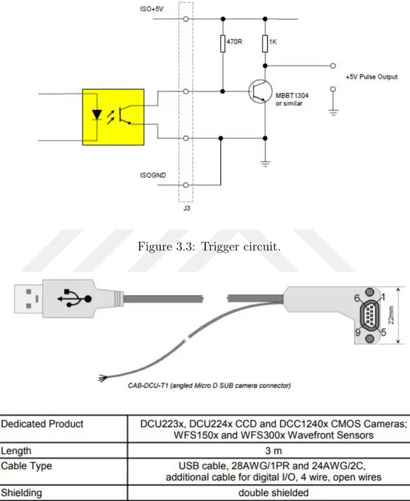
3.4 Trigger cable schematic. . . 20

4.1 Simulation to demonstrate sub-exposure image extraction. (a) Original images, each with size 1280 × 1024 pixels. (b) Zoomed-in regions (13 × 10 pixels) from the masks applied to the origZoomed-inal images. (c) Simulated image capture. (d) Fourier transform (mag-nitude) of the captured image, with marked sidebands used to extract the exposure images. (e) A subset of extracted sub-exposure images. (All 12 images can be successfully extracted; only four of them are shown here.) . . . 23 4.2 Sub-exposure image extraction with FDMI. (a) Recorded

exposure-coded image, (b) Fourier transform (magnitude) of the recorded image, (c) Sub-exposure image recovered from the hori-zontal sideband, (d) Sub-exposure image recovered from the ver-tical sideband, (e) Sub-exposure image recovered from the right diagonal sideband, (f) Sub-exposure image recovered from the left diagonal sideband. . . 25 4.3 Spatial resolution of the optical system. (a) Image without any

optical modulation of the SLM, (b) Extracted sub-exposure image when the SLM pattern is vertical square wave with one-pixel-on one-pixel-off SLM pixels. . . 26 4.4 FDMI experiment with the prototype system, showing recorded

image. . . 28 4.5 FDMI experiment with the prototype system, showing extracted

images. . . 29 4.6 FDMI experiment with the prototype system - Space varying motion. 30 4.7 FDMI with the prototype system - Moving ball. . . 31

LIST OF FIGURES xi

4.8 FDMI experiment with the prototype system - Moving planar

sur-face. . . 32

4.9 FDMI experiment with the prototype system - Optical flow based sub-exposure image extraction. . . 33

4.10 Spatial-domain time division multiplexed imaging. . . 35

4.11 FDMI. . . 36

4.12 Spatial-domain time division multiplexed imaging. . . 37

Chapter 1

Introduction

1.1

Computational Camera

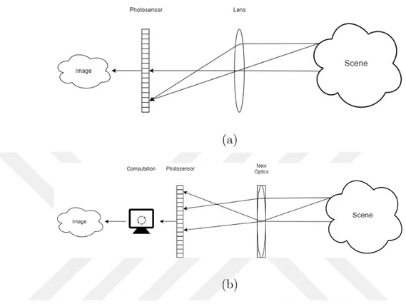
In a conventional camera, a lens forms a two-dimensional projection of a scene on an image plane. The projected image is recorded by means of a film or a semiconductor sensor, which can be based on charged coupled device (CCD) or complementary metal-oxide-semiconductor (CMOS) technology. This basic camera design (consisting of an optical part and an image plane) has not changed since the first camera design, the camera obscura.

A computational camera uses advanced and novel optics, and computational techniques to produce a final image [1]. The optical elements in a computational camera can be used to modulate or redirect the light rays on the desired pixels, in-stead of directly recording them, hence coding the image optically. The captured signal may require a decoding process to extract a two-dimensional projection (a regular image) of the scene as well as additional information about the scene. The decoding process may involve different computational techniques, specifically designed to work with the coded images. Computational cameras may have fixed optics as well moving parts, controlled by programmable micro-controllers or logic devices.

(a)

(b)

Figure 1.1: Traditional and computational camera illustration.

Another way to record a coded image is to use coded illumination. For this purpose, the traditional function of camera flash, which was to illuminate the scene, is modified to project complex illumination patterns to code the scene. The corresponding coded image is captured and then decoded to form an image. There are different coding techniques to make a computational camera. In the next section, two of the main coding techniques, coded aperture and coded exposure, are discussed. An illustration of a traditional and computational camera is shown in Figure 1.1.

1.2

Computational Coding Techniques

1.2.1

Coded Aperture

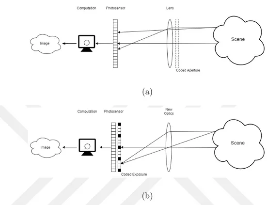
In coded aperture photography, the shape of the aperture plays a vital role. The aperture shapes are designed according to their specific goals in photography. An illustration of coded aperture is shown in Figure 1.2(a). Depth-from-defocus methods incorporate specifically designed apertures to help with depth estimation [2]. In the depth-from-defocus idea, different depths have scaled versions of the aperture shape as defocus blur. By designing the aperture shape, it is possible to distinguish different blur scales easily compared to a standard circular aperture. Furthermore, the depth information can be used to create an all-in-focus image of the scene. This idea has been further explained by adjusting the zero crossings of the point spread function to improve deblurring performance [3]. Depending upon the deblur quality, a detailed framework for determining aperture pattern has been brought forward. The defocus kernel (i.e., the aperture pattern) has a strong impact on the quality of the delurred image. A pattern chosen on the basis of frequency domain has to satisfy that the transmitted values are in 0 to 1 range. The pattern fills the aperture space of the lens and does not induce strong diffractions. The algorithm [3] optimally minimizes the L2 distance between the ground truth and the deblurred image. Coded apertures can be implemented on multiple images, each image with a different coded aperture. These multiple images can be used to acquire light field image [4]. With a traditional camera, a 2D projection of a 3D scene in obtained. The depth information of the scene is lost; but with a 4D light field imaging system, the scene geometry can be preserved and can be processed later for more information from a single capture. To obtain a light field through aperture control method, a non-refractive programmable aperture mask is placed at the camera aperture location. An optimal multiplexing scheme has been introduced [4] through pattern scrolls and liquid crystal array to tackle issues that can be faced in acquiring the light field. Multiple images obtained through coded aperture have also been used in depth estimation and deblurring [5]. In [5], two images are taken with coded aperture hence attaining

broad depth of field and also achieving a well-focused image of the scene. Coded apertures have also been used to perform lensless imaging [6, 7]. In these systems, coded apertures are used to guide light, hence do not require the optical systems to be calibrated.

1.2.2

Coded Exposure

In coded exposure photography, exposure patterns are designed and implemented in order to encode an image during an exposure period. The idea is illustrated in Figure 1.2(b). The exposure pattern can be a global pattern, where all the pixels are exposed simultaneously with a temporal pattern; or a pixel-wise pattern, where each pixel has its own exposure pattern. An example of global exposure coding is the “flutter shutter” technique [8]. Traditionally, the aperture is open for the whole exposure time but in the flutter shutter technique, the aperture is opened and closed in a fast alternating sequence. The sequence is designed in such a way that the point spread function has a maximum coverage in the Fourier domain. The flutter shutter idea can also be used for high-speed imaging [9], where the exposure is coded temporally using an irregular sequence; as a result, high speed motion videos are reconstructed using robust deconvolution algorithms inspired from compressive sensing. Further control of exposure takes place in pixel-wise exposure control, where the exposure of each pixel is controlled, presenting more flexibility and wider range of applications compared to global exposure coding. An example of pixel-wise exposure control is presented in [10], where the goal is to spatially adapt the dynamic range of the captured image. An optical mask, with the help of an liquid crystal (LC) spatial attenuator, is introduced into the optical setup. The LC attenuator controls the exposure of the pixels. The exposure values are adjusted by the attenuator based on a real-time algorithm, to prevent over-exposed regions in the image. Pixel-wise coded exposure imaging can also be used for focal stacking through moving the lens during the exposure period [11], and for high-dynamic-range video through per pixel exposure offsets [12].

Pixel-wise exposure control is also used for high-speed imaging by extracting sub-exposure images from a single capture. In [13], pixels are exposed according to a regular non-overlapping pattern on the space-time exposure grid. Some spa-tial samples are skipped in one time period to take samples in another time period to improve temporal resolution. In other words, spatial resolution is traded off for temporal resolution. In [14], there is also a non-overlapping space-time exposure sampling pattern; however, unlike the global spatial-temporal resolution trade-off approach of [13], the samples are integrated in various ways to spatially adapt spatial and temporal resolutions according to the local motion. For fast moving regions, fine temporal sampling is preferred; for slow moving regions, fine spatial sampling is preferred. Instead of a regular exposure pattern, random patterns can also be used [15, 16, 17]. In [15], pixel-wise random sub-exposure masks are used during exposure period. The reconstruction algorithm utilizes the spatial corre-lation of natural images and the brightness constancy assumption in temporal domain to achieve high-speed imaging. In [16, 17], the reconstruction algorithm is based on sparse dictionary learning. While learning-based approaches may yield outstanding performance, one drawback is that the dictionaries need to be re-trained each time a related parameter, such as target frame rate, is changed.

Alternative to arbitrary pixel-wise exposure patterns, it is also proposed to have row-wise control [18] and translated exposure mask [19, 20]. In [18], instead of traditional rolling shutter, row-wise coded exposure pattern is proposed. The row-wise exposure pattern can be designed to achieve speed imaging, high-dynamic-range imaging, and adaptive auto exposure. In [19], binary transmission masks are translated during exposure period for exposure coding; sub-exposure images are then reconstructed using an alternating projections algorithm. The same coding scheme is also used in [20], but a different image reconstruction approach is taken.

Pixel-wise exposure control can be implemented using regular image sensors with the help of additional optical elements. In [10], an LCD panel is placed in front of a camera to spatially control light attenuation. With such a system, pixel-wise exposure control is difficult since the LCD attenuator is optically defocused. In [21], an LCD panel is placed on the intermediate image plane, which allows

(a)

(b)

Figure 1.2: Illustrations of coded aperture and coded exposure imaging. better pixel-by-pixel exposure control. One disadvantage of using transmissive LCD panels is the low fill factor due to drive circuit elements between the liquid crystal elements. In [22], a digital micromirror device (DMD) reflector is placed on the intermediate image plane. DMD reflectors have high fill factor and high contrast ratio, thus they can produce sharper and higher dynamic range images compared to LCD panels. One drawback of the DMD based design is that the micromirrors on a DMD device reflect light at two small angles, thus the DMD plane and the sensor plane must be properly inclined, resulting in “keystone” perspective distortion. That is, a square DMD pixel is imaged as a trapezoid shape on the sensor plane. As a result, pixel-to-pixel mapping between the DMD and the sensor is difficult. In [23], a reflective liquid crystal over silicon (LCoS) spatial light modulator (SLM) is used on the intermediate image plane. Because the drive circuits on an LCoS device are on the back, high fill factor is possible as opposed to the transmissive LCD devices. Compared to a DMD, one-to-one pixel correspondence is easier with an LCoS SLM; however, the light efficiency is

not as good as the DMD approach. In [19], a lithographically patterned chrome-on-quartz binary transmission mask is placed on the intermediate image plane, and moved during exposure period with a piezoelectric stage for optical coding. This approach is limited in terms of the exposure pattern that can be applied.

1.2.2.1 Frequency Division Multiplex Imaging

Frequency Division Multiplex Imaging (FDMI) is an exposure coding method which demonstrates a sub-exposure image extraction idea. The idea is presented by Gunturk and Feldman as a conference paper [24], where two images are modu-lated with horizontal and vertical square waves. Two optical modulation methods are used, including glass mask and liquid crystal display (LCD) mask. After the patterns are super-imposed on each other, an image is captured in full exposure time. The original images are then extracted from the modulated image using band-pass filtering in frequency domain. While the idea of FDMI is explained in that paper, the capture of sub-exposure images is not presented. In this research, we apply the FDMI idea to extract sub-exposure images using an optical setup incorporating an LCoS SLM synchronized with a camera for exposure coding.

Chapter 2

Frequency Division Multiplexed

Imaging

In this chapter, the method of frequency division multiplexed imaging (FDMI) is explained. Since the method is inspired from the frequency division multiplex-ing (FDM) technique of communication systems, we briefly describe the FDM technique. We, then, discuss the space-time coding of images, followed by FDMI technique with mathematical derivations. In the end, we describe the prototype imaging system used to implement the FDMI technique.

2.1

Frequency Division Multiplexing

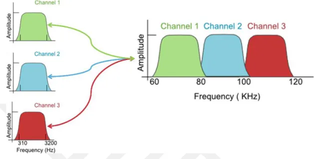
Frequency division multiplexing (FDM) is a communication method of sending multiple data signals on a common channel to a receiver. The data is encoded into a carrier signal. It is ensured that the carrier signal frequencies do not overlap spectrally. A modulator and a demodulator is required at the sending and receiving ends of the communication channel. The modulator encodes the data to be sent and the demodulator uses a band-pass filter to decode the signal received. An illustration of the FDM technique is shown in Figure 2.1.

Figure 2.1: FDM illustration, retrieved from computernetworkingsimplied.in.

2.2

Space-Time Coded Imaging

Space-time exposure coding of an image can be formulated using a spatio-temporal video signal I(x, y, t), where (x, y) are the spatial coordinates and t is the time coordinate. This signal is modulated during an exposure period T with a mask m(x, y, t) to generate an image:

I(x, y) = Z T

0

m(x, y, t)I(x, y, t)dt. (2.1) The mask m(x, y, t) can be divided in time into a set of constant sub-exposure masks: m1(x, y) for t ∈ (t0, t1), m2(x, y) for t ∈ (t1, t2), ..., mN(x, y) for t ∈

(tN −1, tN), where N is the number of masks, and t0 and tN are the start and end

times of the exposure period. Incorporating the sub-exposure masks mi(x, y) into

equation (2.1), the captured image becomes I(x, y) = N X i=1 mi(x, y) Z ti ti−1 I(x, y, t)dt = N X i=1 mi(x, y)Ii(x, y), (2.2)

where we define the sub-exposure image Ii(x, y) =

Rti

ti−1I(x, y, t)dt. The above

equation states that the sub-exposure images Ii(x, y) are modulated with the

(a) (b) (c) (d)

Figure 2.2: Illustration of different exposure masks. (a) Non-overlapping uniform grid exposure [14], (b) Coded rolling shutter [18], (c) Pixel-wise random exposure [16], (d) Frequency division multiplexed imaging exposure [24].

sub-exposure image extraction is to estimate the images Ii(x, y) given the masks

and the recorded image.

As we have already mentioned in Section 1, the reconstruction process might be based on different techniques, varying from simple interpolation [13] to dictionary learning [17]. The masks mi(x, y) can be chosen in different ways as well. Some

of the masks, including non-overlapping uniform grid [13], coded rolling shutter [18], pixel-wise random exposure [16], and frequency division multiplexed imaging exposure [24], are illustrated in Figure 2.2.

Figure 2.3: Illustration of the FDMI idea with two images [24].

2.3

Frequency Division Multiplexed Imaging

The frequency division multiplexed imaging (FDMI) idea [24] is inspired from frequency division multiplexing method in communication systems, where the communication channel is divided into non-overlapping sub-bands, each of which carry independent signals that are properly modulated. In case of the FDMI, sub-exposure images are modulated such that they are placed in different regions in Fourier domain. By ensuring that the Fourier components of different sub-exposure images do not overlap, each sub-sub-exposure image can be extracted from the captured signal through band-pass filtering. The FDMI idea is illustrated for two images in Figure 2.3. Two band-limited sub-exposure images I1(x, y) and

I2(x, y) are modulated with horizontal and vertical sinusoidal masks m1(x, y)

and m2(x, y) during exposure period. The masks can be chosen as raised cosines:

m1(x, y) = a + bcos(2πu0x) and m2(x, y) = a + bcos(2πv0y), where a and b are

positive constants with the condition a ≥ b so that the masks are non-negative, that is, optically realizable, and u0 and v0 are the spatial frequencies of the

masks. The imaging system captures sum of the modulated images: I(x, y) = m1(x, y)I1(x, y) + m2(x, y)I2(x, y).

The imaging process from the Fourier domain perspective is also illustrated in Figure 2.3. Iˆ1(u, v) and ˆI2(u, v) are the Fourier transforms of the

Figure 2.4: The FDMI prototype.

In Figure 2.3, the Fourier transforms ˆI1(u, v) and ˆI2(u, v) are shown as

cir-cular regions. The Fourier transforms of the masks are impulses: Mˆ1(u, v) =

aδ(u, v) + (b/2)(δ(u - u0, v) + δ(u + u0, v)) and ˆM2(u, v) = aδ(u, v) +

(b/2)(δ(u, v - v0) + δ(u, v + v0)). As a result, the Fourier transform ˆI(u, v) of

the recorded image I(x, y) includes ˆI1(u, v) and ˆI2(u, v) in its sidebands, and

ˆ

I1(u, v) + ˆI2(u, v) in the baseband. From the sidebands, the individual

sub-exposure images can be recovered with proper band-pass filtering. From the baseband, the full-exposure image I1(x, y) + I2(x, y) can be recovered with a

low-pass filter.

It is possible to use other periodic signals instead of a cosine wave. For example, when a square wave is used, the baseband is modulated to all harmonics of the main frequency, where the weights of the harmonics decrease with a sinc function. Again, by applying band-pass filters on the first harmonics, sub-exposure images can be recovered.

2.4

FDMI Prototype

The prototype system of FDMI is designed using an LCoS based spatial light modulator (SLM), that is adopted in several papers [23, 16, 17]. LCoS is a reflective micro-display which can alternate the polarization of the impacted ray of light. In this prototype, LCoS is preferred over Liquid Crystal Display (LCD) and DMD because of its higher brightness contrast and high resolution. Furthermore, the loss of light and diffraction in LCoS is much less compared to LCD. LCD lacks in these qualities because its electronic components block light while on the other hand all the electronic components of an LCoS are behind the reflective surface making its fill factor higher than LCD.

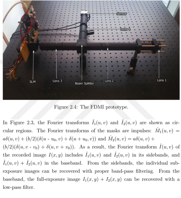
In Figure 2.4, the system consists of an objective lens, three relay lenses, one polarizing beam splitter, an LCoS SLM and a camera sensor. Relay lenses are aspherical doublet lenses of 100mm focal length (ThorLabs, AC254-100-A-ML), 1” cube polarizing beam splitter (ThorLabs), Forth Dimension Display SXGA-3DM 1280x1024 pixels resolution LCoS SLM of sensor size 20.68x18.87mm with 13.62µm pixel width and a ThorLabs DCU-224M camera that is 1/2inch sensor CMOS, 1280x1024 pixels with 4.65µm pixel width. The camera exposure start is synchronized with the SLM using a trigger from the SLM. The camera is set at 40ms and 45ms exposure times, that is, 25Hz and 22Hz respectively; the SLM is set at 40Hz and 45Hz for two kinds of experiments. The optical magnification in the prototype is kept 1:1, but as the pixel sizes in the SLM and the camera sensor are different, there is a magnification of about 2.93. In Figure 2.6, it is seen that a checkerboard pattern of one SLM pixel size is sensed as a three by three pixel region by the camera sensor. This shows that there is about a three times magnification of each SLM pixel.

Figure 2.5: Graphical illustration of the FDMI prototype.

Figure 2.6: A zoomed-in region of the recorded image when the SLM pattern is a one-by-one pixel checkerboard pattern.

Chapter 3

Hardware Assembly

3.1

Overview

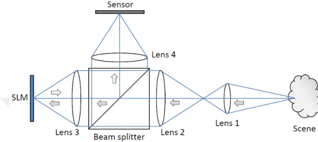
The optical setup is composed of four lenses, a Liquid Crystal over Silicon (LCOS) spatial light modulator (SLM), one polarizing beam splitter and a CMOS camera. This prototype is an exposure controlled 4F optical system. The objective lens focuses the incident light from infinity at its focal point. The first relay lens is focused at the back focal point of the objective lens. The first relay lens and the second relay lens are separated by a combined total distance of both focal lengths. Between these two relay lenses, a polarizing beam splitter is incorporated. The second relay lens in turn focuses the light on the SLM, which is placed at its focal distance; hence both lenses form an exposure controlled 4F optical setup. The light which is refracted through the polarizing beam splitter is polarized into polarization states of S or P . The SLM modulates the incident polarized light according to the modulation pattern. Here, the modulation means that the state of the light is changed from P to S or from S to P . After modulation, the modulated light is deflected by the polarized beam splitter to the third relay lens, while the unmodulated light is refracted through it.The third relay lens is also at a focal distance from both the relay lens one and two. This lens focuses the deflected light from the beam splitter on the sensor of the CMOS camera.

The image on the camera sensor and the SLM sensor is the same image, the only difference being the cropping factor, which occurs due to the difference in pixel sizes of the sensors.

The prototype has been built on a Thorlabs optical table. The lenses and sensors are connected with tubes to prevent side illumination. The tubes are of standard SM 1 size and fit directly to the lenses. To avoid further bent in the path of the light, the tubes are supported by lens and tube supporters. The objective lens and camera are strengthened using rods. With the help of these rods the objective lens and camera are moved swiftly to adjust for minor focal shifts. The tubes, rods and connectors are standard size SM 1 as well. The SLM is mounted on an XY plane translation stage. With the help of the stage, micrometer level adjustment is possible for better focusing between the camera sensor and the SLM. For the SLM, a custom holder is designed and constructed to keep the SLM in place and stable. This custom holder is then connected to the translation stage of the SLM. Sensitive trigger cables, SLM connectors and camera connectors are protected from pull forces by mounting them properly to the optical table.

3.2

Optical Elements

Stronger lenses could be preferred to make the design smaller; however, that would increase aberrations and vignetting effects. The quality of results can further be improved, if the aberrations are reduced. With less aberrations, higher spatial frequencies could be achieved, resulting in better image quality.

The exposure is controlled by focusing the incident light first on the SLM and then reflected light from SLM on the camera sensor. Although the lenses are of same focal lengths, due to the size difference of the SLM and the camera sensor, there is a magnification difference. The camera sensor is smaller than the SLM sensor, therefore a 2.93 times magnification is observed, as mentioned in the previous chapter.

The relay lenses are based upon the 4F system. As the name suggests, the combined system length is two focal lengths, which are the two front focal lengths and two back focal lengths. The incident ray entering the first relay lens focuses rays at one focal distance behind it and is collected by the second relay lens at one front focal distance. This creates a region of plane waves between the first and second relay lenses. Physical spatial filtering can also be applied in this Fourier space.

3.3

Trigger Synchronization

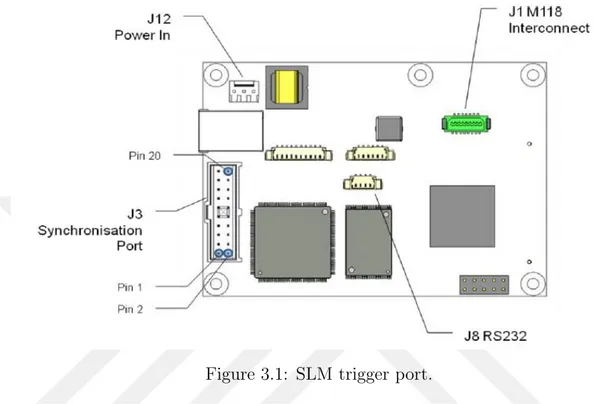
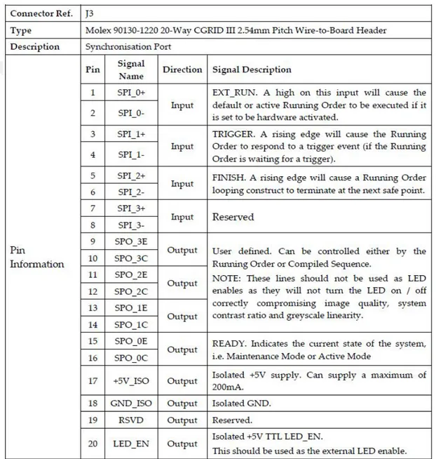
Camera exposure start is synchronized with a trigger signal from the SLM. The SLM configuration can set a trigger to the maximum period of 45 microseconds. The trigger from the SLM is set active for the maximum cycle time. This allows enough exposure time for the camera to capture sufficient data from the scene. The SLM has four trigger output ports, which will be shown later in this section. The SLM switches liquid crystals at 45 millisecond time intervals; in the first 45 milliseconds, the desired modulation patterns are displayed on the LCoS display as positive bit; in the second 45 milliseconds, the negative of those bits are taken to display the compliment of the pattern. This process is called the DC balancing of the liquid crystals. Camera exposure time is also set at 45 milliseconds, to be in sync with the SLM. Due to the synchronization of the triggers of the SLM and camera, the camera will only capture light at its sensor when the trigger from the SLM is set at a rising or active state. Therefore, only the positive bits of the displayed patterns on the SLM are captured. The SLM has a dedicated port for input and output trigger. The block diagram of trigger port in the SLM is shown in Figure 3.1. In the figure, the J3 port is used for trigger purpose. Further details of this port is given in Figure 3.2.

For the prototype, Pin 11 and 12 given in Figure 3.2 are used. These pins correspond to the output trigger pins, labeled as SPO 2E and SPO 2C, respec-tively. The trigger out from the SLM cannot be directly fed as an input to the camera trigger input; for this purpose, a TTL trigger circuit is designed for the

Figure 3.1: SLM trigger port.

trigger synchronization process. The circuit diagram is given in Figure 3.3. The pulsating voltage is given as an input to the camera through trigger cable. The camera trigger cable configuration is shown in Figure 3.4. The “Trigger In” and “Trigger GND” cables are used for the triggering purpose; they are shown as white and brown cables, respectively, in Figure 3.4.

Figure 3.3: Trigger circuit.

Chapter 4

Experimental Results

Several experiments are conducted to demonstrate sub-exposure image extraction with FDMI idea and for traditional spatial methods. The exposure time of the camera is set to 45 milliseconds for FDMI and 40ms for spatial method. For FDMI, in the first 30 millisecond period, the SLM pattern is a square wave in horizontal direction; in the second 15 millisecond period, the SLM pattern is a square wave in vertical direction. For spatial method, in the first 20ms the SLM pattern a black and white checkerboard and in the second 20ms a white and black checker board pattern. The square wave on the SLM is set to its highest possible spatial frequency; that is, one pixel black (no reflection) and pixel white (full reflection). Because of the pixel size difference, one SLM pixel corresponds to an about three by three camera sensor pixels. It is, however, not necessary to detect/extract SLM pixels from the recorded image since the FDMI method only requires applying a band-bass filter to the recorded image.

4.1

FDMI Experiments

4.1.1

Simulation

As the first experiment, we performed a simulation to discuss about the mask design and limitations of the FDMI approach. An image is rotated and translated to create twelve images. Each image is low-pass filtered to obtain band-limited signals. The images are then modulated, each with a different mask, to place them in different regions of the Fourier domain. The masks are designed such that the sidebands at the fundamental frequencies and the harmonics do not overlap in the Fourier domain. We first decide on where to place the sideband in the Fourier domain; form the corresponding 2D raised cosine signal (mask); and discretize (sample) the signal to match size of the input images. Since sampling is involved during the mask creation, we should avoid aliasing. The highest frequency sinusoidal mask (in, for instance, horizontal direction) becomes a square wave (binary pattern) with a period of two pixels.

The original images and zoomed-in regions from the masks are shown in Figure 4.1(a) and Figure 4.1(b), respectively. The highest frequency masks in horizontal and vertical directions are square waves. The modulated image, obtained by multiplying each image with the corresponding mask and then averaging, is shown in Figure 4.1(c). Its Fourier transform is shown in Figure 4.1(d), where the placement of different sub-exposure images can be seen. The baseband and the sidebands from which the sub-exposure images are extracted are also marked in the figure. From these sidebands, we extract all 12 sub-exposure images. Four of the extracted sub-exposure images are shown in Figure 4.1(e).

4.1.2

Experiment with the Prototype

The second experiment is realized with the prototype system. As shown in Figure 4.2, a planar surface with a text printed on is moved in front of the camera. There are four sub-exposure masks: horizontal, vertical, right diagonal and left

(a) (b)

(c) (d)

(e)

Figure 4.1: Simulation to demonstrate sub-exposure image extraction. (a) Orig-inal images, each with size 1280 × 1024 pixels. (b) Zoomed-in regions (13 × 10 pixels) from the masks applied to the original images. (c) Simulated image cap-ture. (d) Fourier transform (magnitude) of the captured image, with marked sidebands used to extract the sub-exposure images. (e) A subset of extracted sub-exposure images. (All 12 images can be successfully extracted; only four of them are shown here.)

diagonal. (These masks are illustrated in Figure 2.2(d).) The exposure period for each mask is 10 milliseconds. The captured image is shown in Figure 4.2(a). Its Fourier transform is shown Figure 4.2(b). The recovered sub-exposure images are shown in Figures 4.2(c)-(d). It is seen that the blurry text in the full-exposure capture becomes readable in the sub-exposure images.

In the experiment, the SLM pattern in horizontal and vertical directions has the highest possible spatial frequency; that is, pixel-on (full reflection) one-pixel-off (no reflection) SLM pattern. In other words, we cannot push the side-bands further away from the center in Figure 4.2(b). The reason why we have an extended Fourier region is that one SLM pixel (13.62µm) corresponds to about three sensor pixels (each with size 4.65µm). If we had one-to-one correspondence, the horizontal and vertical sidebands would appear all the way to the end of the Fourier regions because we have one-on one-off binary pattern for them. To en-code and extract more sub-exposure images, the sub-exposure images should be passed through an optical low-pass filter to further reduce the frequency extent.

4.1.3

Resolution Quantification

The spatial resolution of the optical system is controlled by several factors, includ-ing the lens quality, SLM and sensor dimensions. Since the optical modulation is done by the SLM pixels, SLM pixel size is the main limiting factor of the spatial resolution on the sensing side. On the computational side, the FDMI technique requires band-limited signals, which is also a limiting factor on spatial resolu-tion. In the first experiment, the radius of a band-pass filter used to recover a sub-exposure image is about one-ninth of the available bandwidth, as seen in Figure 4.1; that is, the spatial frequency is reduced to one-ninth of the maximum available resolution as a result of the FDMI process. In the second experiment, the radius of the band-pass filters is about one-fourth of the available bandwidth; that is, the spatial resolution is reduced to one-quarter of the maximum spatial resolution. It should, however, be noted that the bandwidth of a natural image is typically small; therefore, the effective reduction in spatial resolution is not as

(a) (b)

(c) (d)

(e) (f)

Figure 4.2: Sub-exposure image extraction with FDMI. (a) Recorded exposure-coded image, (b) Fourier transform (magnitude) of the recorded image, (c) Sub-exposure image recovered from the horizontal sideband, (d) Sub-Sub-exposure image recovered from the vertical sideband, (e) Sub-exposure image recovered from the right diagonal sideband, (f) Sub-exposure image recovered from the left diagonal sideband.

(a) (b)

Figure 4.3: Spatial resolution of the optical system. (a) Image without any optical modulation of the SLM, (b) Extracted sub-exposure image when the SLM pattern is vertical square wave with one-pixel-on one-pixel-off SLM pixels.

much in practice.

To quantify the overall spatial resolution of our system, we took two photos of a Siemens Star, one without any optical modulation of the SLM (that is, full reflection), and the other with an SLM pattern of maximum spatial frequency (one-pixel-on one-pixel-off SLM pixels). The images are shown in Figure 4.3. The radii beyond which the radial lines can be distinguished are marked as red circles in both images. According to [25], the spatial resolution is (Number of cycles for the Siemens Star) × (Image height in pixels) / (2π(Radius of the circle)). It turns out that the resolution of the optical system (without any SLM modulation) is 138 line width per picture height; while it is 69 line width per picture height for the sub-exposure image. The reduction in spatial resolution is 50%, which is expected considering the spatial frequency of the SLM pattern.

4.1.4

Resolution Test

In this experiment, the scene shown in Figure 4.4(a), is modulated with the SLM into vertical and horizontal line gratings of 30ms and 15ms respectively, that are vertical and horizontal square wave patterns of one SLM pixel thick. These

modulations form a modulated image of scene as shown in Figure 4.4(c). The camera sensor is set at exposure time of 45ms and the total modulation time of the SLM is also 45ms. This results one baseband image and two sideband images in the Fourier domain, shown in Figure 4.4(d). From the Fourier transform, the band-limited components are extracted with bandpass filtering. The original image is recovered from the baseband as if there was no optical mask. The baseband image is identical to the original unmodulated image. The band-limited images can be clearly seen as separate frequency band peaks. These sub-exposure images are extracted from the Fourier transform of the modulated image using bandpass filtering.

The extracted images are shown in Figure 4.5. It is seen that the horizontal sideband, given in Figure 4.5(e), captures a sharp image of the fast moving object; whereas, the vertical subband, given in Figure 4.5(c), maintains a decent spatial resolution with a slight increase in temporal resolution compared to the baseband image.

4.1.5

Extended Resolution Test

In this experiment, shown in Figure 4.6, the whole scene is in motion instead of an object moving in the scene. The same modulation parameters are used as in the previous experiment. From the sidebands, sharper images are recovered, demonstrating the spatio-temporal enhancement.

4.1.6

High Speed Ball

In this experiment, a high speed ball is thrown in front of the camera sensor. The modulation is kept the same for as in the previous case, that is 30ms for verti-cal gratings and 15ms for horizontal gratings, making a total of 45ms exposure time. Using the FDMI technique the sideband images are extracted, as shown in Figure 4.7. Central band or low frequency image obtained has the unmodulated

(a) Original image

(b) Zoomed regions of original unmodulated image

(a) Baseband extracted image and zoomed-in regions

(b) Image extracted from the 30ms vertical grating and zoomed-in regions

(c) Image extracted from the 15ms horizontal grating and zoomed-in regions Figure 4.5: FDMI experiment with the prototype system, showing extracted images.

(a) Recorded image and its Fourier transform

(b) Baseband extracted image and zoomed-in regions

(c) Image extracted from the vertical grating and zoomed-in regions

(d) Image extracted from the horizontal grating and zoomed-in regions Figure 4.6: FDMI experiment with the prototype system - Space varying motion.

(a) Recorded image (b) Baseband image

(c) 30ms sub-exposure image (d) 15ms sub-exposure image Figure 4.7: FDMI with the prototype system - Moving ball.

image, Figure 4.7(b). The vertical band image, Figure 4.7(c), has higher spa-tial resolution but lower temporal resolution than the horizontal grating image. The horizontal grating image, Figure 4.7(d), has captured the fast moving ball because of its higher temporal resolution.

4.1.7

Arbitrary Motion Text

In this experiment, shown in Figure 4.8, a planar surface is moved in front of the camera. The image is degraded with space varying motion blur. The modulation is 30ms for the vertical grating and 15ms for the horizontal grating. Using the FDMI technique, the baseband and the sideband images are extracted. In the 15

(a) Recorded image (b) Baseband image

(c) 30ms sub-exposure image (d) 15ms sub-exposure image

Figure 4.8: FDMI experiment with the prototype system - Moving planar surface. millisecond sub-exposure image, the text becomes readable.

4.1.8

Trajectory Estimation

It is possible to estimate optical flow vectors between two sub-exposure images generated by the FDMI technique, and then use these vectors to estimate more sub-exposure images. The idea is illustrated in Figure 4.9.

(a) Recorded image (b)Fourier transform

(c)Two sub-exposure images and their flow vectors

(d) Intermediate frames obtained by interpolating the optical flow vectors. Figure 4.9: FDMI experiment with the prototype system - Optical flow based

4.2

Time-Division

Multiplexing

and

FDMI

Comparison

In this section, we compare the FDMI technique with the spatial-domain time division multiplexing, where a pixel is exposed only in a sub-exposure period. A checkerboard pattern is used for time division multiplexing of pixels. A scene with still resolution pattern is generated. An object is moved in foreground of this scene, with the same blur effect for both frequency and spatial domain. For the spatial domain imaging, the scene is modulated with the SLM into two alternating checkerboard patterns of one by one pixels.

The checkerboard pattern alters the SLM’s pixel state to active and non-active at every 20ms. The total exposure time of the camera is 40ms. In the first 20ms period, even pixels will be active and in the second 20ms period, the odd pixels will be active, resulting in two sub-exposure images. These images are then interpolated to the original size of 1024x1280 pixels. The images are shown in Figure 4.10.

The same experiment is repeated for the FDMI technique. The scene is modu-lated with the SLM into vertical and horizontal lines gratings, modumodu-lated at 20ms intervals. The total xposure time of 40ms. This results in the formation of two sub-exposure images. Fourier transform of the modulated image is taken. From the Fourier transform, the band-limited components are extracted with bandpass filtering. The original image is recovered from the baseband. The baseband image is identical to original image. The sub-exposure images are extracted from the Fourier transform of the modulated image using bandpass filtering. The images are shown in Figure 4.11.

Since the sampling rate is higher in the spatial domain image, it should produce higher spatial resolution than the FDMI technique. This can be observed when the images in Figure 4.10 and Figure 4.11 are compared carefully. The drawback of the spatial domain technique should occur when the signal-to-noise ratio is low. The overall exposure time for a pixel is higher in the Fourier domain technique

(a) Original image (b) Coded image

(c) Recovered from the first half of the exposure

(d) Zoomed-in region of (c)

(e) Recovered from the sec-ond half of the exposure

(f) Zoomed in region of (e)

Figure 4.10: Spatial-domain time division multiplexed imaging.

compared to the spatial domain technique. Also, we need to investigate what happens if the entire scene is in motion. As a final experiment, the whole scene is set into motion instead of an object moving in the scene. The results for spatial domain technique and the FDMI technique can be seen in Figure 4.12 and Figure 4.13. It is observed that the spatial resolution is effected drastically if the whole scene is in motion. Sub-exposure images using the FDMI technique seem to be sharper than the ones obtained from the spatial domain technique.

(a) Original image (b) Coded image (c) Fourier transform of (b)

(d) Baseband image (e) Zoomed in region of (d)

(f) Image extracted from the vertical sideband

(g) Zoomed in region of (f)

(h) Image extracted from the horizontal sideband

(i) Zoomed in region of (h)

(a) Original image (b) Coded image

(c) Recovered from the first half of the exposure

(d) Zoomed in region of (c)

(e) Recovered from the sec-ond half of the exposure

(f) Zoomed in region of (e)

(a) Unmodulated original image

(b) Coded image (c) Fourier transform of (b)

(d) Baseband image (e) Zoomed-in region of (d)

(f) Image extracted from the vertical sideband

(g) Zoomed-in region of (f)

(h) Image extracted from the horizontal sideband

(i) Zoomed in region of (h)

Chapter 5

Conclusions

In this thesis, we demonstrate a sub-exposure image extraction method, which is based on allocating different regions in Fourier domain to different sub-exposure images. We demonstrate the feasibility of the idea with real life experiments using a prototype imaging system. The imaging system has physical limitations due to low spatial resolution of the SLM and low light efficiency, which is about 25%. Better results would be achieved in the future with the development of high-resolution sensors allowing pixel-wise exposure coding.

An advantage of the proposed approach is the low computational complex-ity, which involves Fourier transform and bandpass filtering. The sub-exposure images from the sidebands and the full exposure image from the baseband are eas-ily extracted by taking Fourier transform, bandpass filtering, and inverse Fourier transform.

Extraction of sub-exposure images can be used for different purposes. In addi-tion to high-speed imaging, one may try to estimate space-varying moaddi-tion blur, which could be used in scene understanding, segmentation, and space-varying deblurring applications.

Bibliography

[1] S. K. Nayar, “Computational cameras: Redefining the image,” Computer, vol. 39, no. 8, pp. 30–38, 2006.

[2] A. Levin, R. Fergus, F. Durand, and W. T. Freeman, “Image and depth from a conventional camera with a coded aperture,” ACM Trans. on Graphics, vol. 26, no. 3, p. Article No. 70, 2007.

[3] C. Zhou and S. Nayar, “What are good apertures for defocus deblurring?,” in IEEE Int. Conf. on Computational Photography, pp. 1–8, 2009.

[4] C.-K. Liang, T.-H. Lin, B.-Y. Wong, C. Liu, and H. H. Chen, “Programmable aperture photography: multiplexed light field acquisition,” in ACM Trans. on Graphics, vol. 27, p. Article No. 55, 2008.

[5] C. Zhou, S. Lin, and S. K. Nayar, “Coded aperture pairs for depth from defocus and defocus deblurring,” Int. Journal of Computer Vision, vol. 93, no. 1, pp. 53–72, 2011.

[6] Y. Sekikawa, S.-W. Leigh, and K. Suzuki, “Coded lens: Coded aperture for low-cost and versatile imaging,” in ACM SIGGRAPH, 2014.

[7] M. S. Asif, A. Ayremlou, A. Veeraraghavan, and R. Baraniuk, “Flatcam: Replacing lenses with masks and computation,” in IEEE Int. Conf. on Com-puter Vision, pp. 12–15, 2015.

[8] R. Raskar, A. Agrawal, and J. Tumblin, “Coded exposure photography: motion deblurring using fluttered shutter,” ACM Trans. on Graphics, vol. 25, no. 3, pp. 795–804, 2006.

[9] J. Holloway, A. C. Sankaranarayanan, A. Veeraraghavan, and S. Tambe, “Flutter shutter video camera for compressive sensing of videos,” in IEEE Int. Conf. on Computational Photography, pp. 1–9, 2012.

[10] S. K. Nayar and V. Branzoi, “Adaptive dynamic range imaging: Optical con-trol of pixel exposures over space and time,” in IEEE Int. Conf. on Computer Vision, pp. 1168–1175, 2003.

[11] X. Lin, J. Suo, G. Wetzstein, Q. Dai, and R. Raskar, “Coded focal stack photography,” in IEEE Int. Conf. on Computational Photography, pp. 1–9, 2013.

[12] T. Portz, L. Zhang, and H. Jiang, “Random coded sampling for high-speed hdr video,” in IEEE Int. Conf. on Computational Photography, pp. 1–8, 2015.

[13] G. Bub, M. Tecza, M. Helmes, P. Lee, and P. Kohl, “Temporal pixel multi-plexing for simultaneous high-speed, high-resolution imaging,” Nature Meth-ods, vol. 7, no. 3, pp. 209–211, 2010.

[14] M. Gupta, A. Agrawal, A. Veeraraghavan, and S. G. Narasimhan, “Flexi-ble voxels for motion-aware videography,” in European Conf. on Computer Vision, pp. 100–114, 2010.

[15] D. Reddy, A. Veeraraghavan, and R. Chellappa, “P2c2: Programmable pixel compressive camera for high speed imaging,” in IEEE Int. Conf. on Com-puter Vision and Pattern Recognition, pp. 329–336, 2011.

[16] Y. Hitomi, J. Gu, M. Gupta, T. Mitsunaga, and S. K. Nayar, “Video from a single coded exposure photograph using a learned over-complete dictionary,” in IEEE Int. Conf. on Computer Vision, pp. 287–294, 2011.

[17] D. Liu, J. Gu, Y. Hitomi, M. Gupta, T. Mitsunaga, and S. K. Nayar, “Efficient space-time sampling with pixel-wise coded exposure for high-speed imaging,” IEEE Trans. on Pattern Analysis and Machine Intelligence, vol. 36, no. 2, pp. 248–260, 2014.

[18] J. Gu, Y. Hitomi, T. Mitsunaga, and S. Nayar, “Coded rolling shutter pho-tography: Flexible space-time sampling,” in IEEE Int. Conf. on Computa-tional Photography, pp. 1–8, 2010.

[19] P. Llull, X. Liao, X. Yuan, J. Yang, D. Kittle, L. Carin, G. Sapiro, and D. J. Brady, “Coded aperture compressive temporal imaging,” Optics Express, vol. 21, no. 9, pp. 10526–10545, 2013.

[20] R. Koller, L. Schmid, N. Matsuda, T. Niederberger, L. Spinoulas, O. Cos-sairt, G. Schuster, and A. K. Katsaggelos, “High spatio-temporal resolution video with compressed sensing,” Optics Express, vol. 23, no. 12, pp. 15992– 16007, 2015.

[21] C. Gao, N. Ahuja, and H. Hua, “Active aperture control and sensor mod-ulation for flexible imaging,” in IEEE Int. Conf. on Computer Vision and Pattern Recognition, pp. 1–8, 2007.

[22] S. K. Nayar, V. Branzoi, and T. E. Boult, “Programmable imaging: Towards a flexible camera,” Int. Journal of Computer Vision, vol. 70, no. 1, pp. 7–22, 2006.

[23] H. Mannami, R. Sagawa, Y. Mukaigawa, T. Echigo, and Y. Yagi, “High dynamic range camera using reflective liquid crystal,” in IEEE Int. Conf. on Computer Vision, pp. 1–8, 2007.

[24] B. K. Gunturk and M. Feldman, “Frequency division multiplexed imaging,” in IS&T/SPIE Electronic Imaging Conf., pp. 86600P–86600P, 2013.

[25] C. Loebich, D. Wueller, B. Klingen, and A. Jaeger, “Digital camera res-olution measurement using sinusoidal Siemens Stars,” in SPIE Electronic Imaging, Digital Photography III, pp. 65020N1–11, 2007.