Efficiency of Istanbul Stock Exchange with respect to macroeconomic variables: a study using Granger causality

♦ t T V « - J i H 6

5706-5

o U

W!th Н^^зоэсі То у ас

/-^ S’lijc!\/

З'С—ас^а···“

EFFICIENCY OF

ISTA N BU L STOCK EXCHANGE

WITH RESPECT TO MACROECONOM IC VARIABLES:

A STU D Y U SIN G GRANGER C A U SA LIT Y

A THESIS

SUBMITTED TO THE DEPARTMENT OF MANAGEMENT

AND THE GRADUATE SCHOOL OF BUSINESS ADMINISTRATION

OF BILKENT UNIVERSITY

IN PARTIAL FULFILLMENT OF THE REQUIREMENTS

FOR THE DEGREE OF MASTER OF BUSINESS ADMINISTRATION

By

MUMJ-OZEK--.

/P / '

H

5 4 0 b - 5

. A2>

о з ц

I certify that I have read this thesis and it is fully adequate, in scope and in quality, as a thesis for the degree o f Master o f Business Administration.

Assist. P ıradoğlu

I certify that I have read this thesis and it is fully adequate, in scope and in quality, as a thesis for the degree o f Master o f Business Administration.

Assist. Prof Kıvılcım Metin

I certify that I have read this thesis and it is fully adequate, in scope and in quality, as a thesis for the degree o f Master o f Business Administration.

Assist. Prof. Fatma Taşkın

Approved for the Graduate School o f Business Administration.

O '

ABSTRACT

EFFICIENCY OF

ISTANBUL STOCK EXCHANGE

WITH RESPECT TO MACROECONOMIC VARIABLES: A STUDY USING GRANGER CAUSALITY

MURAT ÖZER

M.B.A.

Supervisor: Assist.Prof.Giilnur MURADOGLU

June, 1996

The purpose o f this study is to test the efficiency o f Turkish security market with respect to a

number o f macroeconomic variables, using multivariate Granger causality tests in conjunction

with Akaike's final prediction error(FPE) criterion. The data set includes the daily values o f the

Istanbul Exchange Index and macroecononomic variables between the years 1988-1994. The

testing period is divided into sub-periods, based on the levels o f trading volume which represents

the different developmental phases o f the market. The empirical results showed that the

macroeconomic variables effecting the stock prices change through time, in accordance to the

changing market characteristics. Therefore, the success o f any model over the estimation period

does not guarantee that the same model will perform well outside the testing period.

Keywords: Stock market efficiency. Granger causality. Macroeconomic variables. Developing

ÖZET

İSTANBUL MENKUL KIYMETLER BORSASI’NIN MAKROEKONOMÎK DEĞİŞKENLERE GÖRE ETKİNLİĞİ:

BİR GRANGER NEDENSELLİK ÇALIŞMASI

MURAT ÖZER

Yüksek Lisans Tezi, İşletme Enstitüsü

Tez Yöneticisi: Doç. Dr. GÜLNUR MURADOĞLU

Haziran 1996

Bu çalışmanın amacı, Türk Hisse Senedi Piyasası'nın makroekonomik değişkenlere göre

etkinliğini, Akaike'nin minimum tahmin hatasına ile beraber çok değişkenli Granger

nedensellik testi yardımyla ölçmektir. Kullanılan veri kümesi, 1988 ve 1994 yılları

arasında, günlük İstanbul Menkul Kıymetler Borsası kapanış endeksi ve makroekonomik

değişkenlerin değerlerini kapsamaktadır. Veri kümesinin ait olduğu dönem, piyasanın

gelişme düzeylerine bağlı olarak, değişen işlem hacmi seviyelerine göre alt dönemlere

ayrılmıştır. Ampirik sonuçlar hisse senedi fiyatlarını etkileyen makroekonomik

değişkenlerin, değişen piyasa özeliklerine göre, zaman içinde farklılık gösterdiğini ortaya

koymaktadır. Buna bağlı olarak, tahmin döneminde başarılı olan bir modelin, bu dönem

dışında da başarıya ulaşması konusunda yargıya ulaşmak mümkün değildir.

Anahtar Kelimeler: Hisse Senedi Piyasası Etkinliği, Granger Nedenselliği, Macroekonomik

ACKNOWLEDGEMENTS

I would like to express my gratitude to Assist. Prof. Giilnur Muradoğlu for her guidance,

support and encouragement for the preparation o f this thesis. I would like to thank my other

thesis committee members Assist. Prof Kıvılcım Metin and Assist. Prof Fatma Taşkın for

their valuable comments and suggestions. I would also like to thank all the members o f the

Department o f Management o f Bilkent University for providing me this MBA education.

LIST OF TABLES

Table 1. Summary o f Empirical Studies Investigating the Relationship Between the Stock Prices and MacroeconomicVariables... 5-6

Table 2. Number o f lags for Augmented Dickey-Fuller tests...26

Table 3a. Results o f Dickey-Fuller Tests at Log Levels... 27

Table 3b. Results o f Dickey-Fuller Tests at Log Differences...28

Table 4. Autocorrelation Analysis for the First Differenced Logarithmic

Stock Price Series... 29.

Table 5. Basic Statistical Properties for the Stock Prices and Macroeconomic

Data at Log Differences between 1988-1994...30

Table 5a. Basic Statistical Properties for the Stock Prices and Macroeconomic

Data at Log Differences between 1988-1989...30

Table 5b. Basic Statistical Properties for the Stock Prices and Macroeconomic

Data at Log Differences between 1990-1992... 30

Table-5c. Basic Statistical Properties for the Stock Prices and Macroeconomic

TABLE OF CONTENTS

INTRODUCTION...1

LITERATURE REVIEW... 4

2.1. General Empirical Research... 5

2.2. Empirical Research on Turkish Market... 14

METHODOLOGY... 17

3.1. Theoretical Framework... 17

3.2. Stationarity... 18

3.2.1. Augmented Dickey-Fuller Tests... 19

3.3. Distributional Properties o f Data...21

3.3.1. Autocorrelation Analysis... 21

3.3.1.1. Ljung-Box Q Portmanteau Statistic...22

3.3.2. Normality Tests... 22

3.4. Testing Granger Causality... 23

DATA...27

EMPIRICAL RESULTS... 29

4.2. Stationarity... 29

4.2.1. Determining the Lag Order(for ADF tests)... 30

4.2.2. Augmented Dickey-Fuller Tests...32

4.3. Distributional Properties o f the Log Differenced Series... 33

4.4. Testing Granger Causality... 36

4.5. Discussion o f the Results... 39

REFERENCES... 46

APPENDIX I. GRAPHS OF STOCK PRICES AND MACROECONOMIC

VARIABLES OVER THE PERIOD 1988-1994...48

APPENDIX II. GRAPHS OF STOCK PRICES AND MACROECONOMIC

VARIABLES AT LOG LEVELS OVER THE PERIOD 1988-1994... 54

APPENDIX III. DETERMINATION PROCEDURE OF THE LAG

LENGTHS FOR ADF TESTS... 60

APPENDIX IV. GRAPHS OF STOCK PRICES AND MACROECONOMIC

VARIABLES AT LOG DIFFERENCES OVER THE PERIOD 1988-1994...63

APPENDIX V. AUTOCORRELATION ANALYSIS OF THE LOG

DIFFERENCED TIME-SERIES... 69

APPENDIX VI. RESULTS OF SEQUENTIAL MODEL REDUCTION

I. INTRODUCTION

There exists a great deal o f literature which tests the Efficient Market Hypothesis. In its

semistrong form, the Efficient Market Hypothesis states that stock prices fully reflect all

publicly available information. Two types o f semi-strong form efficiency test can be

conducted, one using micro data such as company-specific announcements, the other with

macro data such as money stock, interest rates, inflation (Groenewold & Kang, 1993). With

a few exceptions, information about macroeconomic variables have been ignored in the

efficient market literature, especially for the stock markets o f developing countries.

However, in the thinly-traded stock markets o f the developing countries where government

intervention to the economy is a common practice, the macroeconomic variables has a

crucial role in the formation o f stock prices (Muradoglu & Onkal, 1992).

Only a limited number o f empirical studies are conducted on the rapidly developing

Istanbul Stock Exchange which tested the efficiency with respect to macro economic

variables.( Erol and Aydoğan,1991, Muradoğlu and Önkal-1992, Muradoğlu and Metin-

1995,1996). This study will analyze the market efficiency in Türkiye by investigating

empirically the relationship between the daily stock returns in Istanbul Stock Exchange

and a number o f macroeconomic variables, which are expected to influence the stock

returns. The variables included in the model are the money stock, the interest rates and the

exchange rates in Türkiye. These variables form an important set o f information for the

The efficient market hypothesis contends that there should be no significant lagged

relationship between the stock prices and the publicly available information in the semi­

strong sense. In the recent literature, multivariate Granger causality tests are one o f the

most common techniques for testing the semi-strong efficiency. (Darrat and

Mukherjee: 1986, Darrat: 1988,1990) The aim o f this study is to test the efficiency o f

Istanbul Stock Exchange, applying multivariate Granger causality tests along with Akaike's

final prediction error(1969) to find out any significant lagged relationship between the

stock returns and the set o f macroeconomic variables included in the model.

The stock market data and macroeconomic data belong to the period 1988-1994. The

testing period is divided into sub-periods, considering the different developmental phases

o f the stock market, based on the volume o f trade in Istanbul Stock Exchange. In the first

sub-period (1988-1989), the firm-specific information flow was poor, market participants

were few and volume o f trade was low. In the second sub-period (1990-1992), the volume

o f trade increased mainly by the entrance o f foreign and domestic institutional investors to

the stock market. In the last sub-period (1993-1994), the volume o f trade reached to a

considerable amount and both the number o f individual and institutional participants

increased (Muradoglu and Metin, 1996). The empirical testing procedure is applied to

subsequent periods to find out any change in the stock price equation in the above market

phases and find indications o f any development in the market efficiency in the semi-strong

sense.

This study is organized as follows: In the first chapter, the introduction is done focusing on

second chapter. In the third chapter, the theoretical framework is established discussing the

relation between the Efficient Market Hypothesis and Granger causality and also the

method that will be used in the empirical study is explained. Fourth chapter belongs to the

description o f data. The empirical results and discussion o f the results are given in the fifth

chapter. In the conclusion chapter, comments are made about the results o f the study and

Efficient-Market hypothesis has extensive inferences for both the theory and practice o f

finance and economics. Therefore, it is not surprising that it has been broadly tested by

various methods, using data for different assets, countries and different time periods

(refer to Table 1).

In the literature, a distinction is made between three potential levels o f efficiency. Under

the weak form o f efficiency, the information on historical price movements is fully

absorbed by the future stock prices and they have no value in predicting the price

development. There exists semi-strong form o f efficiency in the security market if the

movements in security prices can not be predicted on the basis o f publicly available

information. And finally, a stock market is said to be efficient in strong form; if the

security prices reflect all the relevant information including the data not yet publicly

available (Virtanen and Yli-Olli, 1986). 2. LITERATURE REVIEW

One aspect o f the empirical literature is noteworthy. While there exist numerous empirical

studies testing the efficiency o f the developed capital markets, only a sparse number o f

studies exist for the stock markets in developing countries. One reason which causes in less

attention to be given to these markets could be that many investors in developed countries

avoid LDC's markets due to high perceived risk associated with investment in these

countries arising largely from political uncertainties. However, though the total risk o f

holding securities in these markets is rather high, the risk in the portfolio context may be

important reason for ignoring LDC's markets might be that in many cases they have been

inaccessible for the international investors(Darrat and Mukherjee, 1986). However, recently

things seem to be changing rapidly in this regard. With the internationalization o f the

financial markets, the capital markets o f the LDC's are receiving increased attention from

the investors and academicians.

7'he capital markets o f the developing countries display specific characteristics that must be

considered during empirical studies. In these countries, the trading volume o f the capital

markets is relatively low and the share o f the state in financial and economic activity is

high, so the government policies have an important effect on the capital markets. Also, the

firm-specific publicly available information is usually limited and delayed.(Muradoglu &

Onkal, 1992). Therefore, the macroeconomic variables representing the monetary and fiscal

actions o f the government is expected to shape the expectations o f the investors and have a

crucial role in the formation o f stock prices.

2.1. General Empirical Research

The globalization trend in the financial markets requires the empirical studies on the LDC's

markets to be done on a comparable base with the studies on the capital markets o f the

developed countries. In Table-1, the recent studies that contributed to the efficient market

research by investigating the relationship between the security prices and the

TABLE I

Suinman of Empirical Studies Investigating the Relationship Between the Stock Prices and Macroeconomic Variables

Author(s) Year o f Study Country' Sample Data Sample Period Differencing Intern al of the stock prices

Support market efficiency? Pearce and Roley 1983 U.S. Stock market aggregates, announced changes in money and e.xpected money 1977-82 weekly Yes Pearce and Roley 1985 U.S. Stock market aggregates, money stock, price level(CPI & PPI), industrial

production index, unemployment rate, discount rates

1977-79 1980-82

daily Yes

Darrat and Mukhejee 1986 India Stock market aggregates, money stock, short-term & long-term interest rates, aggregate demand(GNP), price level

1948-84 annually No

Leiderman and Offenbacher 1986 Israel Stock market aggregates, announced monetary injections & change in the stock o f foreign currency reserves

1982-85 daily No

Jones and Uri 1986 U.S. Stock market aggregates and money stock 1974-83 monthly Yes

Virtanen and Yli-olli 1987 Finland Stock market aggregates, aggregated future cash flow of firms, interest rates, money stock, inflation, other stock market aggregates

1975-84 monthly and quarterly

No

Hardouvelis 1987 U.S. Stock market aggregates. 15 announced macroeconomic variables 1979-82 1982-84

daily No

Hashemzadeh and Taylor 1988 U.S. Stock market aggregates, money stock, interest rates 1980-86 weekly No

Darrat 1988 Canada Stock market aggregates, money stock, unemployment rate, balance of payments, short-term interest rates, inflation and aggregate demand(GNP)

1960-84 quarterly No

Asprem 1988 10 European

Countries

Stock market aggregates o f ten countries, industrial production, exchange rates, imports, exports, interest rates, inflation and money stock, employment figures

1968-84 quarterly No

Hancock 1989 U.S. Stock market aggregates, money stock, inflation rate, unemployment rate, budget deficit, 3 month T-bill rate, government securities held abroad, aggregate demand(GNP)

1960-85 quarterly Yes

Darrat 1990 U.S. Stock market aggregates, privately held federal debt, 3 months T-Bill rate, GNP deflator, real GNP, a proxy for risk premium, non-fmancial corporate profits

1961-87 quarterly No

Darrat 1990 Canada Stock market aggregates, money stock, budget deficits, long&short-term interest rates, industrial production, volatility' o f interest rates, inflation rate and exchange

1972-87 monthly Yes

TABLE 1 (Continued)

Mcqueen and Rolcy 1993 U.S. _{Stock market aggregates, discount rate proxies, industrial production,} unemployment rate, nonfarm payroll employment, merchandise trade deficit, inflation rate(CPl & PPI). money stock, expected values o f the variables

1977-88

daily-All and Hasan 1993 Canada _{Stock market aggregates, money stock, high-employment budget deficit, price}

level(CPI). interest rates, exchange rates. US money stock and stock returns 1970-88 monthly Yes Grocnewold and Kang 1993 Australia _{Stock market aggregates, money stock(M3. MO and M6). proxies for government}

expenditure and price level 1982-88 monthly Yes

Muradoğlu and Metin 1995 Türkiye _{Stock market aggregates, budget deficit. 3 moths T-Bill rates, exchange rates,}

inflation rate(CPI). money stock(Ml and M2). 1986-93 monthly No

Muradoğlu, Metin and Argaç 1996 Türkiye _{Stock market aggregates, overnight interest rates, money stock(Ml, M2 and} currency in circulation), exchange rates(U.S. Dollar. German Mark. British Sterling and Japanese Yen)

1988-89 1990-92 1993-95

Pearce and Roley(1983) investigated the response o f the stock prices to weekly money

announcements by using a linear-response model. In examining the response o f the stock

prices, survey data on market's participants' forecasts o f the announced weekly change are

used to distinguish expected from actual changes in money stock The empirical results

indicated that stock prices responded only to unanticipated change in money supply as

predicted by efficient market hypothesis, also an unanticipated increase in the announced

money supply depresses stock prices, while an unanticipated decrease elevates the stock

prices.

In an other study, Pearce and Roley(1985) examined the daily response o f the stock prices

to the announced values o f narrowly defined money stock, the consumer price index, the

producer's price index, the unemployment rate, industrial production and Federal Reserve

discount rate. To represent the new information released by an announcement, they used a

measure o f market expectancy. The results showed that money announcement surprises

have a significant negative effect on stock prices, whereas only limited evidence supports

the view that inflation and real economic activity surprises affect stock prices. As a last

finding, the empirical results indicated that anticipated components o f economic

announcements have no significant effect on stock prices, which is consistent with the

efficient market hypothesis.

Darrat and Mukherjee(1986) investigated the causal relationship between the stock returns

and a set o f macroeconomic variables, applying Granger-type o f causality test to Indian

are found to exercise a significant negative impact upon stock returns suggesting that the

stocks and long term bonds are seen as substitutes. As an other finding, inflation was found

to exert some negative effect on stock returns.

Leiderman and Offenbacher(1986) investigated the responses o f stock prices in Israel to

monetary announcements. Only unexpected part o f the monetary injection announcements

are found to exert a significant positive impact on stock prices, while announcements o f

international reserves are found to have no significant influence on stock prices.

Jones and Uri(1986) employed the Granger direct test to determine the causal relationship

between the stock returns and money supply in US stock market. Their findings

demonstrated that the stock market is efficient in the sense that current and past information

with regard to the money supply is fully absorbed by the cument stock prices, hence

investors are not able to develop profitable trading mles with information about changes in

money supply.

One other empirical study that gives contradicting evidence about the efficient market

hypothesis belongs to Virtanen and Yli-011i(1987). They tested the weak and semi-strong

efficiency o f the Finnish capital market, using the aggregated cash-flows o f firms, interest

rates, money stock, inflation and prices in Swedish stock market. According to the

empirical results o f this study, all the variables included in the models were explanatory o f

the stock prices and the stock market in Finland is neither efficient in semi-strong form nor

While examining the response o f stock prices and interest rates to fifteen macroeconomic

variables, Hardouvelis(1987) focused on the distinction between monetary and non­

monetary news and on the role expected future Federal Reserve behavior might play both

after monetary and non-monetary announcements. In his results, he concluded that stock

prices primarily respond to monetary news. The strongest reactions were observed at a

period when the Federal Reserve followed strict annual M l targets and adopted non-

borrowed reserves as weekly targets. Also, among the non-monetary news stock prices are

found to respond to the announcements o f trade deficit, the unemployment rate and

personal income, implying market inefficiency.

Hashemzadeh and Taylor(1988) investigated the relationship between the money stock and

stock prices and between the interest rates and stock prices. Employing Granger-Sims test

for determining unidirectional causality, they found out that there exists bi-directional

causality which relate stock prices to money stock and vice-versa. Examining the

relationship between the interest rates and stock prices, the results showed that the causality

seems to be mostly running from the interest rates to stock prices without a feedback.

Darrat(1988) investigated empirically the relationships between the aggregate quarterly

stock returns and a set o f macroeconomic variables, based on the monetary and fiscal policy

actions in Canada. He applied the two-step procedure akin to Barro(1977, 1978) for setting

up the stock price equation. In the first step, he estimated an ex-ante equation, based on

unemployment rate and balance o f payments, to forecast Canadian anticipated and

unanticipated fiscal policy moves. Then, in the second step he estimated a stock price

equation using the two measures obtained and other candidate explanatory macro

have a significant effect on current stock returns, indicating market efficiency. However,

the results verified that fiscal policy actions had a significant lagged effect on the stock

returns, contrary to Efficient Market Hypothesis.

Asprem(1989) examined the relationship between the stock indices, asset portfolios and

macroeconomic variables in ten European countries, using OLS regressions and factor

models. The results o f the study indicated that employment, imports, inflation and interest

rates were inversely related to stock prices, whereas expectations about future real activity,

measures o f money and U.S. yield curve were positively related. Also, a portfolio

consisting the stock price indices o f all ten countries is found to explain the stock price

variations most strongly, implying strong linkage between the capital markets. The

macroeconomic variables are shown to be most effective in explaining stock returns for

Germany, Netherlands, Switzerland and U.K. For several relationships, links between the

past values o f macroeconomic variables and current stock returns was detected, suggesting

market inefficiency.

Hancock(1989) tested the semi-strong form o f efficiency hypothesis with respect to

anticipated and unanticipated monetary and fiscal variables, using U.S. quarterly data. As

Darrat(1988), he applied the two step strategy o f Barro(1977,1978). First, he estimated two

equations for the money stock growth and the change in budget deficit, based on a number

o f macro variables. Then, he used the fitted and residual values obtained from the

forecasting equations (representing the anticipated and unanticipated policy actions) with

some other relevant variables to set up a stock price equation. As Tanner and Trapani(1977)

states the EMH allows for the significance o f a contemporaneous unanticipated variable,

but not the significance o f a contemporaneous anticipated variable. Based on this fact, the

empirical results showed that U.S. capital market is efficient with respect to both fiscal and

monetary variables.

Darrat(1990a) tested the semi strong efficiency hypothesis with respect to the stance o f U.S.

fiscal policy. As the previous, studies indicated the efficiency o f the stock prices with

respect to the monetary policy and no significant relationship between the monetary and

fiscal policies(Bamhart and Darrat, 1989) the monetary variables were not included in the

model. While performing the empirical study, Akaike's final prediction error criterion was

combined with multivariate Granger causality tests. The results verified that the fiscal

policy had a significant causal effect on the stock prices during the estimation period. The

likelihood ratio tests, held to check the robustness o f the model, showed that the

coefficients o f the fiscal variable proved to be jointly significant, therefore the causal

relationship could be identified a s " a strong form o f causation".

In an other empirical study, Darrat( 1990b) re-examined the causal relationship between the

changes in Canadian stock returns and a set o f macroeconomic variables. While performing

the empirical analysis. Granger-causality tests in conjunction to Akaike's final prediction

error were used. Consistent with the results o f Darrafs(1988) previous study, the current

stock prices were found to absorb past monetary policy moves. However, as before, the

fiscal policy was found to exercise a significant lagged effect on the Canadian stock returns.

Mcqueen and Roley(1993) examined the relationship between the stock prices and

fundamental macroeconomic news in different stages o f the business cycle. In addition,

they examined effect o f real activity news on proxies for expected cash flows and equity

empirical studies, based on the assumption " stock prices equals the present discounted

value o f rationally forecasted dividends.". The empirical study indicated that the stock

market's response to macroeconomic news depended on the state o f the economic activity.

Specifically, news o f higher-than-expected real activity in a strong economy resulted in

lower stock prices, whereas the same surprise in a weak economy resulted in higher stock

prices. The reason for the variations in response o f stock prices across mentioned economic

states appears to be the expected cash flows.

Ali and Hasan(1993) re-tested the market efficiency o f the Canadian stock market with

respect to monetary and fiscal variables, using the vector autoregression(VAR) technique.

The empirical study, based on the impulse response functions obtained from the moving

average representations o f the VAR model, supported that the Canadian Stock Market is

efficient with respect to both fiscal and monetary variables. The results o f the study found

no support o f inefficiency o f the stock market, contrary to Darrat's(1988) study, which

found evidences o f the stock market inefficiency with respect to government's fiscal policy

actions. Ali and Hasan explained that one o f the reasons for the contradiction could be the

distinction between the models used. They stated; "Indeed, Darrat's(1988) study, based on a

single equation instrum ental variable approach d id take "sufficient care to ensure statistical robustness" o f the m odel, but nevertheless, his m odel was prim arily an em pirical one. In such a m odel, as argued b y Darrat(1988,p.354), it is n ot p o ssib le to analyze the precise channels through which the fiscal p o lic y w ould influence the stock return^'.

Groenewold and Kang(1993) examined the weak and semistrong forms efficiency in

Australian stock market. Since, weak efficiency is a necessary condition for testing

semistrong efficiency, at first, it was tested by three tests, two o f which examining the

intertemporal structure o f the stock returns and the third being a test for unit root in the

price series. After concluding that the market was weakly efficient, semi-strong form o f

efficiency tests were held using regressions based on the unanticipated components o f the

macro variables. A set o f forecasting equations were estimated, two o f which were for real

economic activity, and three for the money supply The results were in favor o f the market

efficiency, as the lagged returns or lagged values o f the unanticipated values o f the

variables had no significant joint explanatory power in regressions.

2.2. Empirical Research on Turkish Stock Market

In Türkiye, there has been only a limited number o f studies testing the semi-strong form o f

efficiency with respect to macroeconomic variables. One o f the pioneering studies was held

by Muradoğlu and 0nkal(1992). They checked the semi-strong form o f efficiency o f

Istanbul Stock Exchange with respect to a number o f macroeconomic variables,

representing the monetary and fiscal actions o f the government. They used Barro's(1978)

two step-strategy. First, they estimated two equations for the fiscal and monetary policy o f

the government. Then, in the second step, they set up two equations for the stock prices for

testing the two conditions o f market efficiency;

1. The effect o f lagged unanticipated & anticipated variables and the contemporaneous

anticipated variables on stock prices should not be significant.

2. The effect o f contemporaneous unanticipated variables on stock prices should be

statistically significant.

The results indicated that stock returns lagged the fiscal policy with two months and the

monetary policy with two months. Also, the effect o f contemporaneous unanticipated

An other study testing the semi strong effieieney o f Istanbul Stoek Exchange with a

different method was held by Muradoğlu and Metin(1995). They used the recently

developed techniques, namely unit roots and cointegration. The results indicated that the

stock prices and monetary variables cointegrate in the long run, thus the stock market is not

efficient with respect to monetary variables. Then, a short-run dynamic model is estimated

and the stock market was found out to assimilate publicly available information on

monetary variables with a lag, thus strengthening the evidence for market inefficiency.

In one o f the most recent studies, Muradoğlu and Metin(1996) re-tested the efficiency o f

Istanbul Stock Exchange Market with respect to monetary variables by using the Engle and

Granger's cointegration technique. Cointegration technique enables us to analyze efficiency

through time by using the information revealed by non-stationary macroeconomic

variables. Although the individual variables o f concern may be non-stationary, if these

variables are cointegrated, their linear combinations can be stationary in cointegrating

relations. When this technique is used, information loss due to differencing is prevented.

Applying the cointegration technique, the first step is regressing the stock prices on the

macroeconomic variables and obtaining OLS regression residuals. At the second step, the

existence o f unit roots in the OLS residuals is tested by using ADF tests. In the case o f no

unit roots, the series are concluded to be cointegrated. If the stock prices and individual or

group o f macroeconomic variables come out to be cointegrated, the stock market is

indicated to be inefficient. By using this technique, efficiency was tested at different

developmental phases o f the market, which was distinguished by different levels o f

transaction volume. The empirical results denoted that stock prices did not cointegrate with

any o f the variables for the whole research period( 1988-1995), indicating market efficiency.

However, this result was not valid for all sub-periods. Dividing the research period into sub

periods, a change in market efficiency is observed through time. The only sub-period that

the stock market seemed to be efficient was the first period(1988-1989) where no

cointegration between the stock prices and macroeconomic variables were detected. In the

second (1990-1992) and third (1992-1995) periods the stock market is determined to be

inefficient. Muradoğlu and Metin(1996) stated that the change in the market efficiency

through various sub-periods arises from the distinct characteristics o f the market structures

and participants.

The empirical research on the efficiency o f the Turkish stock market has been increasing in

number parallel to the developing stock market, however, yet there exists only a few studies

testing the efficiency with a limited number o f methods. This study is expected to

contribute further to the limited efficient market literature in Türkiye, applying a different

method than the previous studies, namely multivariate Granger causality tests. Granger

causality tests are a commonly used methods to determine the lagged relationship between

time-series and have powerful implications for the semi-strong form o f efficiency o f the

3. METHODOLOGY

3.1. Theoretical Framework

The efficient market hypothesis suggests that the lag (if any) between the macroeconomic

variables and stock returns can not be positive at a significant level and can not allow for

the formulation o f trading rules that will result in excess profits( Jones and Uri, 1986). That

means there are no systematic lagged effects between the stock prices and macroeconomic

variables. To conclude that the market is efficient in semi strong sense, the lagged

coefficients o f macroeconomic variable in the stock price model should be statistically

insignificant.

Tests for causality are efficient tools to determine the lagged relationship between the

variables o f concern. In the present context, causality is defined in terms o f predictability.

In this study, a test .for causality attributed to Granger is implemented

Granger causality is an econometric relationship in which additional information from one

time-series helps to explain another series. In setting up a causal model, if the additional

information provided by X helps to explain Y, then the inclusion o f X in the model will

reduce the variance o f Y.

a2(Y/I) < cj2(Y/I-X)

where Y and X are the variables in the sample set, I is the total information set and is the

variance.

In this situation, X is said to Granger-cause Y. Granger causality is based on two

assumptions:

(1) The future can not cause the past. Strict causality can only occur with the past causing

the present or the future.

(2) A cause contains unique information about an effect that is not available elsewhere.

Before conducting Granger causality tests, stock prices and macroeconomic variables data

are examined for stationarity, as in standard Granger causality tests stationary variables

should be used.

3.2. Stationarity

A time-series is defined as stationary, if the stochastic process that generated the time-series

is invariant with respect to time, that is its basic statistical characteristics(e.g. mean and

variance) remain constant. If the characteristics o f a stochastic process change over time,

i.e. if the process is non-stationary, it is difficult to represent the time series over past and

future intervals o f time by an algebraic model. On the other hand, if the stochastic process

is fixed over time, i.e. if the process is stationary, it is possible to model the process via an

equation with fixed coefficients that can be estimated from past data.

In practice, very few o f the time-series are stationary at level. However, many o f the

are differenced one or two times. If a nonstationary time-series can be transformed to a

stationary time-series by differencing, it is called as homogenous.

In this section, the time-series o f macroeconomic variables are investigated for stationarity

by the help o f Dickey-Fuller unit root test and the need for differencing is assessed.

3.2.1. Augmented Dickey-Fuller Unit Root Test

The finding o f a unit root in a time series indicates nonstationarity. Dickey-Fuller unit root

test is developed by David Dickey and Wayne Fuller(1981) to determine the presence o f a

unit root in a time-series. The following model is employed to test the presence o f the unit

root (Pindyck and Rubinfield, 1991):

Suppose a variable Yt, which is growing over time can be described by the following

equation:

Yt = a + pt + pYt-1 + St

, where Yt is the macroeconomic variable, a is the drift variable, p is the trend coefficient,

t is time from t=0 to last observation, st jg the error term.

In this situation, the series Yt may be growing because o f the positive trend o f the series ( P>0) or because o f the positive drift(a>0, p = l, p=0). If there exists a positive trend, the

series can be detrended to reach to stationarity and Yt can be used in a regression model. In

the latter case, where the series follows a random walk with a positive drift, detrending has

no use to reach stationarity and the series requires differencing.

Dickey and Fuller(1981) generated statistics for simple F test o f the random walk

hypothesis, i.e. o f the hypothesis that p=l and P=0. The following test procedure developed

by Kendall(1990) gets use o f this statistic.

Suppose Yt can be described by the following unrestricted equations:

(1) Yt - Yt_i = «0+ ct2Yt-l Lj^Yt-j + St :with-constant, no-trend

(2) Yt - Yt_i = tto + ttit + a2Yt-l + Sj LjAY^.j + st :with-constant, with-trend

The null hypothesis for each equation are;

(1) Ho: Yt is a random walk plus drift, ao= 0, a2= 0

(2) Ho: Yt is a random walk plus drift around a stochastic trend, a i= 0, a2= 0

First, one o f the above unrestricted equations is ran, afterwards the following restricted

equation is ran using ordinary least squares.

(3) Y t - Y t . i - a o + ZjLjAYt.j + st

Then, the standard F-ratio is calculated to test if a i= 0, a2= 0 as follows;

where ESSr and ESSuR are the sums o f squared residuals in the restricted and

unrestricted regressions, N is the number o f observations, k is the number o f estimated

parameters in the unrestricted equation and q is the number o f parameter restrictions.

In testing the null hypothesis, the critical values generated by Dickey and Fuller(1981) are

used rather than the standard F ratio table(Pindyck & Rubinfield, Econometric Models and

Econometric Forecasts)

In addition to this, t-test is employed to test if the condition a i= 0 holds. The t-test is

calculated as;

t(Y,j) = (Y-1) /SE(Y) ,where SE(Y) = standard error o f parameter Y at lag j, J = lag order

3.3. Distributional Properties o f the Time-Series

In this section, the autocorrelation analysis and non-normality tests are conducted for the

time-series after reaching stationarity.

3.3.1 Autocorrelation Analysis

The jth-order autocorrelation coefficient indicates the level o f interdependency between the

observations Yj and Yt+j· The autocorrelation coefficient can also be used to determine

whether a time-series is stationary or not. If Tj (autocorrelation coefficient) does not

diminish rapidly as lag j increases, this indicates nonstationarity.(Pindyck & Rubinfield,

1991,p.449)

The autocorrelation structures o f the macroeconomic time-series both at log levels and log

differences are investigated and Ljung-Box Q portmanteau statistic(1978) is used to pick

up any departures from randomness in the first j autocorrelations.

3.3.1.1 Ljung-Box Q Portmanteau Statistic

In order to test the joint hypothesis that all the autocorrelation coefficients are zero, Ljung-

Box Q statistics is used. The test-statistic is computed as:

Q = N(N+2)Zj(l/N-j)xj2 forj=l,...,p

where N is the number o f observations, x; is the sample autocorrelation coefficient, defined

as;

. xj =Sj+, (yt - y) (yt-j - y)/ S(yt - y f , where y=Syt/T

Under the null hypothesis, Q has an asymptotic xj2 distribution with j and the first j

autocorrelations are zero, which means there exists no lagged dependent variables. If the

null hypothesis is false, the test-statistic tends to become large, thus indicating model

inadequacy.

3.3.2. Normality Tests

In this section, the stock prices and macroeconomic variables, which have reached to

by using coefficient o f kurtosis. The skewness coefficient show deviations from the normal

distribution in either the upper or lower parts o f the distribution, and approaches to zero as

the distribution gets nearer to normality. The kurtosis coefficient provides evidence on

whether the distribution is more or less fat-tailed than expected from the normal

distribution. When the kurtosis is zero, the data is concluded to be normally distributed. The

data departs from normality as the kurtosis ratio gets larger.

3.4. Testing Granger Causality

In this section, a number o f macroeconomic variables, including money stock(M2),

interbank overnight interest rates(INT) and Central Bank exchange rates for German

Mark(DM) and United States Dollar(USD) are used to test to Granger-cause the stock

returns in Istanbul Stock Exchange.

In order to find the causal relationship between the stock returns and the information set o f

macroeconomic variables, the following multi-variate model is employed:

SPt = a + E bj SPt-i + E Cj M2t.j +E dj INT^.j + E f j . E^.j +ei

i = l,...,n

where all the variables are in natural logarithms and daily data o f ISE index ( SPt) over the

years 1988-1994 is used as the dependent variable, whereas the daily money stock (M2t),

overnight interbank interest rates (INTt), exchange rates (Et) including the US dollar and

DM are used as the independent macro variables having the causal effect on the stock

returns.

All variables are lagged from one day to ten days to make the model a predictive one, as our

hypothesis is that there exist a significant lagged relationship between the stock prices and

the macro variables included in the model.

While testing the model indicated above, the macro variables are tested to Granger-cause

the stock returns. The procedure which is employed by Mcmillin & Fackler(1984) and

Darrat & Mukherjee(1987) is used to include the causal variables with the appropriate lag

lengths to the model. This procedure uses the Akaike's final prediction error(FPE) as a

criteria to decide on the causal variables.

In testing the model, stationary data o f all variables is used, which has been differenced

with the required order, found out after conducting unit root tests.

The testing procedure used is as follows:

First, the optimal own lag o f stock prices is determined. This is done by varying the lag in

successive autoregressions o f stock prices. For each autoregression FPE is calculated and

defined for the lag k, k=l,...,10 as:

FPE(k) - {(T+k+l)/(T-k-l)}.(RSS/T)

RSS = sum o f squared residuals

T = number o f observations in time-series

Hsiao(1981) points out that the FPE criterion is equivalent to using an F-test with a varying

significance level. According to Judge et al.(1982), an intuitive reason for using FPE

criterion is that an increase in the lag length increases the first term, but decreases the

second term and these opposing forces are balanced when their product reaches to a

minimum. Thus according to Hsiao(1981), FPE criterion is "... appealing because it

balances the risk due to bias when a low er order is selected and the risk due to the increase o f variance when a higher order is selected."

Once the optimal own lag order(k*) for stock prices is found out, which macroeconomic

variables is to enter the equation is determined next. A number o f bivariate regressions are

ran with the optimal own lag o f stock prices and one o f the other macroeconomic variables,

varying the tag length(n) for the variable, n=l,...,10. The FPE criterion is computed for each

regression as follows:

FPE(k*, n) = {(T+k*+n+l)/(T-k*-n-l)} . (RSS/T)

The lag length that minimizes the FPE criterion is chosen as the lag order(n*) for that

variable. This FPE is compared with the FPE o f the previous step, that is the optimal own

lag o f the stock prices(k*). If FPE(k*, n*) < FPE(k*), then the variable is said to Granger-

cause stock prices and retained in the model for further consideration. If FPE(k*,n*) >

FPE(k*), the variable is discarded from the model.

Among the variables that Granger-cause the stock prices, the variable with the lowest FPE

is added to the model with the lag order obtained from the bivariate regression.

At the third step, a number o f triviate regressions are estimated, by including each o f the

remaining variables in the equation. The FPEs for each regression are computed and

defined for the lag m, m =l,..., 10, as:

FPE(k*,n*,m) = {(T+k*+n*+m+l)/(T-k*-n*-m-l)} . (RSS/T)

As before, the lag length that results in the minimum FPE is chosen as the lag order o f that

variable. This FPE is again compared with the minimum FPE from the bivariate regression.

If FPE(k*,n*,m*) < FPE(k*,n*), then the variable said to Granger-cause stock prices and

retained in the model for further consideration, otherwise it is discarded from the model.

The variable that has the minimum FPE is included in the equation, after the triviate

regressions are ran for each o f the variables.

All remaining variables are tested subsequently to have a causal relationship with the stock

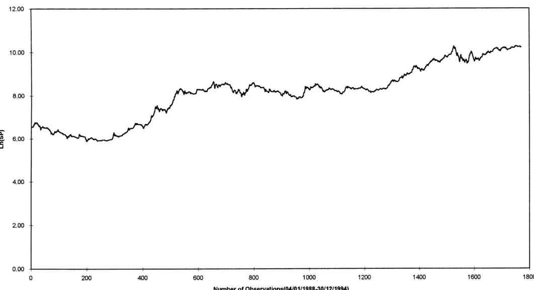
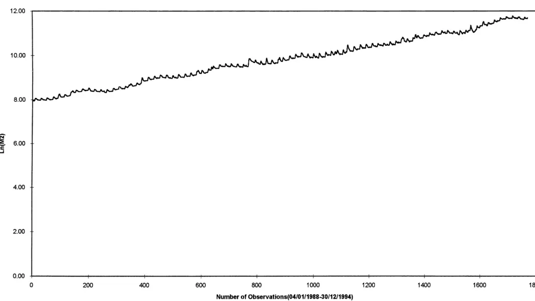
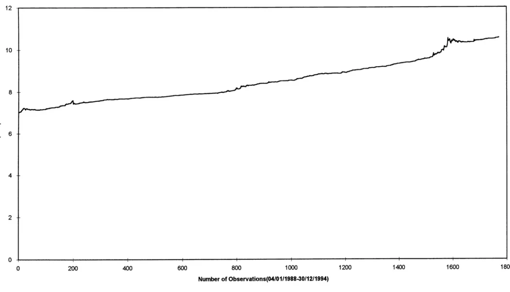
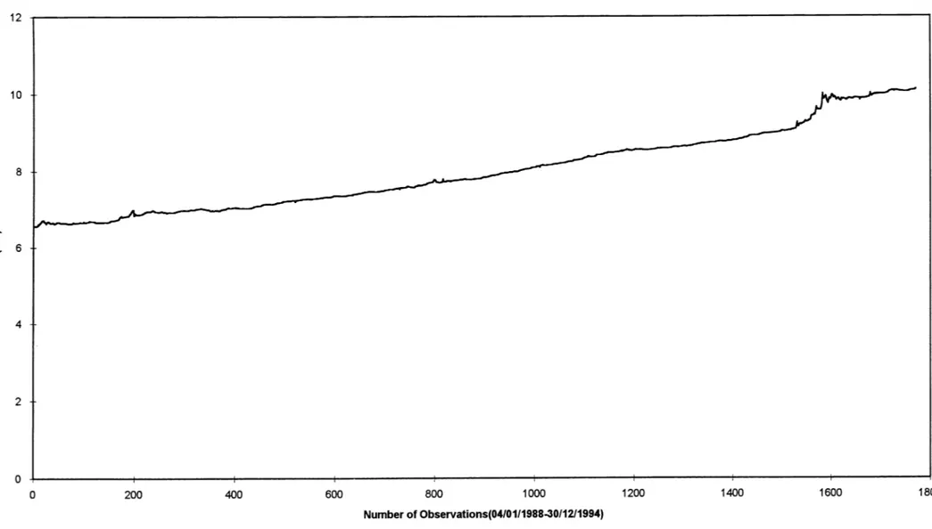
4. DATA

In this study, the data used consists o f the daily values o f a number o f macroeconomic

variables including the composite stock price index o f Istanbul Stock Exchange, to

represent stock prices, the money stock(M2), the interbank overnight interest rates. Central

Bank exchange rates, including German Mark and United States Dollar over the period

beginning in January 4,1988 and ending in December 30,1994. The graphs o f all the time

series are submitted in Appendix 1.

The data set is divided into three sub-periods according to the different developmental

phases o f the stock market, considering large shifts in volume o f trade. The first period

(1988-1989) represents the initial phase o f the market. In this period, the firm-specific

information flow is poor, market participants few and volume o f trade is low. In the second

sub-period( 1990-19920, the volume o f trade increased mainly by foreign and domestic

institutional investors. In the third sub-period (1993-1994), market expansion reached to a

high level by the increase in both the individual and institutional investors.

Natural logarithmic data in levels is used while employing the tests. One o f the reasons for

using natural logarithmic transformations is the non-linearity o f the economic time series.

As it can be seen in most o f the economic time series, the growth is with a roughly constant

percentage, rather than an absolute rate and this can be handled with logarithmic

transformations. An other reason for using logarithmic data is that, when using logarithms,

the efficiency o f the estimates is increased because the heterocedasticity in regression

analysis is reduced as the data is smoothened, therefore in the case o f time series analysis,

stationarity in variance can be achieved (Virtanen & Yli-Olli, 1987). The graphs o f all

4. EMPIRICAL RESULTS

In this chapter, the stationarity properties o f the macroeconomic variables and stock prices

data and the causal model between the stock prices and macroeconomic variables is

discussed.

4.2. Stationarity

Dickey-Fuller unit root tests are run for checking the presence o f a unit root in the stock

prices and macroeconomic variables. Before conducting the Augmented Dickey-Fuller

tests, the appropriate lag order to be included in the test should be calculated for all o f the

time series.

4.2.1 Determining the Lag Order(for ADF tests)

In determining the appropriate lag length for the time series, the following method is used;

First, the autoregression Yt = a + Pi Sj Yt.i + St is run for the time series upto lag 10. The t-

statistic is computed for each lag and the insignificant lags at 95% confidence level are

discarded. Then, an autoregression is run with the remaining lags for the series, the

insignificant lags are again excluded from the model. This procedure is repeated till all the

significant lags in one step, come out to be significant in the next step. The highest

significant lag is chosen as the lag order for the Augmented Dickey-Fuller test.

As an example, the procedure for determining the appropriate lag order for the interest rate

series at log level between the years 1988-1994 is illustrated in Appendix 3. The same

algorithm is applied to all the time series in each period and the results are summarized in

Table-2.

Table-2. Number o f lags for Augmented Dickey-Fuller tests (significance level = 5%) Period ISE Index Money

Stock(M2) Interbank Interest Rates US Dollar German Mark 1988-1994 3 7 8 9 9 1988-1989 3 7 10 1 3 1990-1992 2 7 11* 7 1 1993-1994 3 7 1 4 4

is ran including the next 5 lags, this time the last lag that is significant at 5% level com e out to be 11

4.2.2. Augmented Dickey-Fuller Tests

Augmented Dickey-Fuller Tests are applied to the logarithmic stock price series and

macroeconomic data for two alternative unrestricted models, with constant and no-trend &

Table-3a. Results o f Dickey-Fuller Tests at Log Levels constant, no trend constant, trend

Period Lag

Order

t-statistic F-statistic t-statistic F-statistic

sig.lcvcl= l% sig.lcvcl= l% sig.lcvel= l% sig .lcv cl= l%

crit, val.=-3.43 crit. val.=6.43 crit. val.=-3.96 crit. val.=8.27

1988-1994— Ln(SP) 3 -0.07o013 2.8411 -1.8269 T .8689 Ln(M2) ~1 -0.36401 7.2127* -5.5016* 15.138* Ln(INT) 8 -4.2317* 8.9718* -4.9174* 12.129* Ln(USD) 9 2.0661 23.o91* -0.56559 2.6808 Ln(DM) 9 2.4464 25.571* -0.84o02 "3.9177---1988-1989 Ln(SP) 3 1.3623 2.0007 -0.35297 5.0197---Ln(M2) 7 -0.54093 2.o532 -2.9025 ”4.2214---Ln(INT) 10 -3.1493* 5.0323 -4.6328* 10.789*---Ln(USD) 1 -0.80747 ■0;82566 -2.0979 2.2648 Ln(DM)--- 3 -3.2917* 5.4292 -3.4894* 6.1308 1990-1992— Ln(SP)--- 2 -3.6374* 0.7408* -3.6584 6.9890 Ln(M2) 7 -1.0148 2.7124 -5.1698* 13.377* Ln(INT) 11 -2.6180 3.6414 -2.5584 3.5707 Ln(USD)--- 7 0.74044 T 9.961* “^ .1 7 8 4 --- 2.9093 Ln(DM) 1 0.19129 27.067* -2.5637 3.3820 1993-1994 Ln(SP) 3 -2.0147 4.1394 -2.5338 3.8451 Ln(M2) 7 -0.85993 3.03 84 -3.0813 4.7754---Ln(INT) 1 -3.8562* 7.4462* -3.9512* 7.8157 Ln(USD) 4 -0.24466 6.1303 -1.6124 1.3136 Ln(DM)--- 4 -0.082963 6.6786* -1.6347

1.3957---♦ indicates statistics which arc significant at 1% significance level.

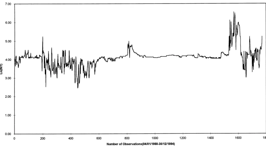
The results justify existence o f a unit root in interest rate series, when referring to the test

statistics for the constant and trend specification. In one o f their recent studies, Muradoglu

and Metin(1996) found that all these series have unit roots for a similar period. The graphs

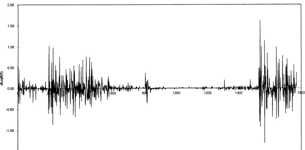
o f all time series(Appendix 2) are examined and it is detected that all the series except

interest rate series show a growing characteristics with respect to time, which is an

indication o f non-stationarity. The interest rate series seem not to be growing through time,

however they show high fluctuations in some periods, which causes non-stationarity by

variance. At this step, all series including stock prices and macroeconomic variables are

subjected to first differencing and the first-differenced series are again tested for unit roots

with the help o f augmented Dickey-Fuller tests. The results are illustrated below(Table-3b)

Table-3b.Results o f Dickey-Fuller Tests at Log Differences constant, no trend constant, trend

Period Lag

Order

t-statistic F-statistic t-statistic F-statistic

sig.lcvel= l% sig.Icvcl= l% sig.lcvcl= l% sig .lcv cl= l%

crit. val.=-3.43 crit. val.=6.43 crit. val.=-3.96 crit. val.=8.27

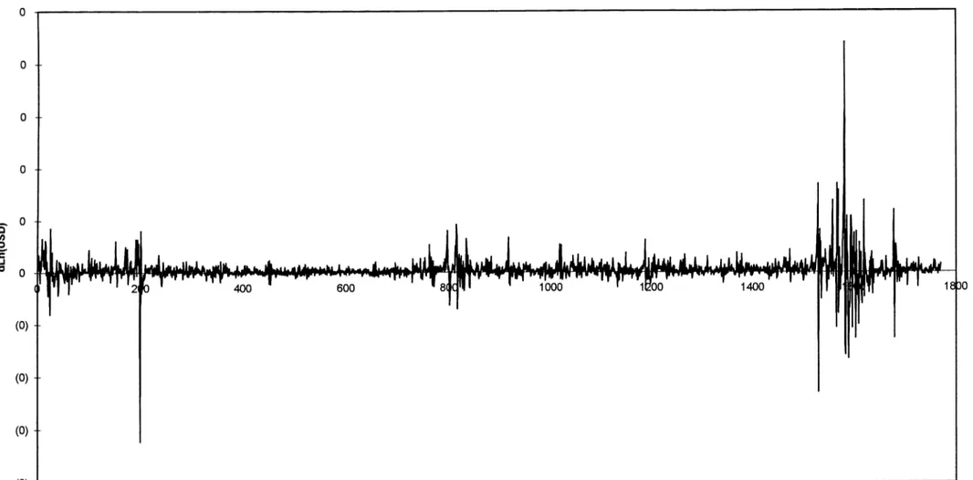
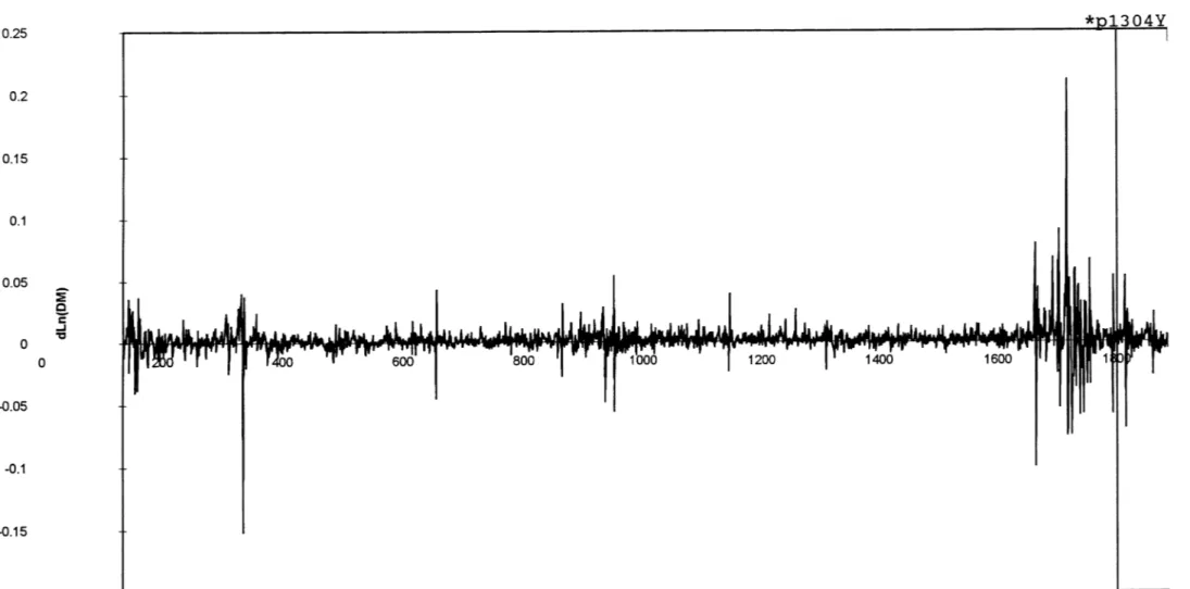
1988-1994 Ln(SP) 3 -22.773’" 259.31’" -22.778’" 259.42=" Ln(M 2) 1 -20.972* 219.92’" -20.966’" 219.92=" T n [I N T ) 8 -20.U55’" 201.11’" -20.050’" 201.03=" L n(U SD ) 9 -15.325* 117.43’" -15.510’" 120.30=" L n(D M ) 9 -15.261* 116.45’" -15.502’" 120.15=" 1988-1989"" Ln(SP) 3 -1 1 .8 9 P 70.757’" -1 2 .4 0 P 76.912=" Ln{M 2) “ 7 -10.839* 58.753’" 1-10.829’" 58.666=" L n d N T ) 10 -9.4U2l’^ 44.204’" -9.400’" 44.192=" Ln(UST5) 1 -15.890* 126.25’" “ 15.880’" 126.09=" L n(D M ) 3 -14.435’*' 104.20’" -14.422··" 104.405=" 1990-1992“ Ln(SP) 2 18.944* 179.45’" " 18.955’" 179.66=" Ln(M21 7 -13.873’*' 96.243’" -1 3 .8 6 P 96.105=" L n d N 'll 11 -13.979’*' 97.76 P -13.984’" 97.941=" LndJST^ 7 -11.388’*' ‘ 64.850’" -11.433’" 65.360=" L n(D M ) 1 -29.577’*' 437.41’" -29.564’" 437.03=" 1993-1994 Ln(SP) 3 -11.532’" 66.495’" -11.587=" 67.130=" Ln(M 2) 7 -11.155’" 62.225’" -11.143=" 62.109=" L n(lN T ) 1 -1 9 .7 5 P 195.10’" :i9.723="--- 194.67=" Ln(USD'5 4 -12.211’" 74.560’" -12.200=*= 74.422=" L n(D M ) 4 -12.U91’" 73.091’" -1 2 .08 5 * 73 022="

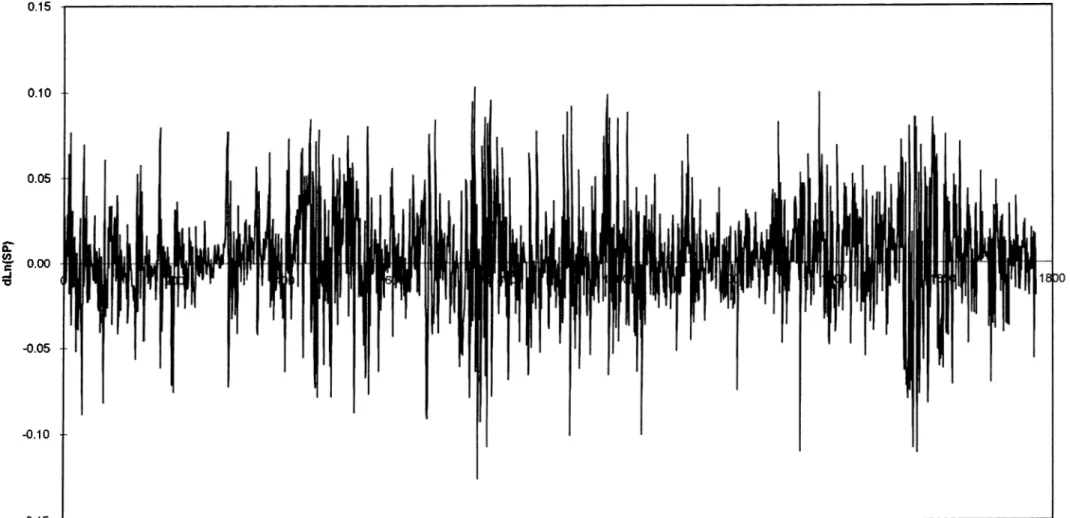
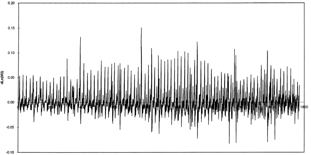
For all o f the first-differenced series, the null hypothesis o f a unit root is rejected at 1%

significance level, as the F-statistics are all greater and the t-statistics are all smaller than

the critical values, therefore stationarity is reached at log differences. The graphs o f the log

differenced series can be seen in Appendix 4.

4.3. Distributional Properties o f the Log Differenced Series

At the next step, the autocorrelation structures o f the log differenced stock prices and

macroeconomic variables is inspected and tests for detecting non-normality o f the series are

held. The autocorrelation coefficients and Ljung-Box Q Statistics are computed for the log

differenced series and submitted in Appendix 5. As an example, the autocorrelation analysis

o f stock price series at log differences can be seen below:

Table-4. Autocorrelation Analysis for the Log Differenced Stock Price Series for the Period 1988-1994

Lag Autocorrelation Coefficient Box-Ljung Q Statistic P-Value 1 0.01 0.30 0.587 2 0.00 0.30 0.861 3 0.00 0.30 0.960 4 0.00 0.30 0.990 5 0.00 0.32 0.997 6 0.00 0.35 0.999 7 0.00 0.36 8 0.01 0.53 9 0.00 0.55 10 0.00 0.59 33

It can be seen that the autocorrelation coefficients are aproximately zero. The joint

hypothesis that all autocorrelation coefficients are zero can not be rejected, as the Ljung-

Box Q Statistics are not significant at 1% level.

Next, the basic statistical properties for the log differenced series are examined. The data is

investigated for skewness and kurtosis.

Table-5. Basic Statistical Properties for the Stock Prices and Macroeconomic Data at Log Differences between 1988-1994

iSE index Money Stock interest Rate US Doilar German Mark Coefficient of Skewness -0.02914 1.323895 1.03686 1.841946 1.732843 Coefficient of Kurtosis 1.26446 3.172812 19.30945 81.94585 65.46721 Mean 0.002078 0.002098 0.00064 0.002002 0.002012 Median 0.000773 -0.00281 0 0.001202 0.0013 Mode 0 0 0 0 0 Standard Deviation 0.030274 0.025587 0.158248 0.012505 0.012689 Maximum 0.102681 0.150518 1.61222 0.219859 0.210777 Minimum -0.12591 -0.08254 -1.29541 -0.16089 -0.15138

Table-5a. Basic Statistical Properties for the Stock Prices and Macroeconomic Data at Log Differences between 1988-1989

iSE Index Money Stock Interest Rate US Dollar German Mark Coefficient of Skewness 0.077741 1.681056 0.682826 -7.58632 -5.85743 Coefficient of Kurtosis 1.148332 5.134055 5.266224 128.496 89.12363 Mean 0.001946 0.002067 -0.00105 0.001067 0.001028 Median 0.000448 -0.0018 0 0.000768 0.000961 Mode 0 0 0 0 0 Standard Deviation 0.027268 0.0197 0.19886 0.010194 0.010509 Maximum 0.084156 0.131817 1.014722 0.042396 0.03959 Minimum -0.08826 -0.04295 -0.86069 -0.16089 -0.15138