Full Terms & Conditions of access and use can be found at
https://www.tandfonline.com/action/journalInformation?journalCode=hbhf20
The Journal of Behavioral Finance
ISSN: 1542-7560 (Print) 1542-7579 (Online) Journal homepage: https://www.tandfonline.com/loi/hbhf20
A Behavioral Approach To Efficient Portfolio
Formation
Yaz Gulnur Muradoglu , Aslihan Altay-Salih & Muhammet Mercan
To cite this article: Yaz Gulnur Muradoglu , Aslihan Altay-Salih & Muhammet Mercan (2005) A Behavioral Approach To Efficient Portfolio Formation, The Journal of Behavioral Finance, 6:4, 202-212, DOI: 10.1207/s15427579jpfm0604_4
To link to this article: https://doi.org/10.1207/s15427579jpfm0604_4
Published online: 07 Jun 2010.
Submit your article to this journal
Article views: 122
A Behavioral Approach To Efficient Portfolio Formation
Yaz Gulnur Muradoglu, Aslihan Altay-Salih,
and Muhammet Mercan
This paper investigates the portfolio performance of subjective forecasts given in dif-ferent forms. In constructing the efficient frontier, we base the expectation formation processes on subjective forecasts and human behavior, rather than on past prices. We construct the efficient portfolios first, using point, interval, and probabilistic fore-casts. Next, we compare their performance to portfolios constructed using the stan-dard time series data approach. Subjective forecasts are provided by actual portfolio managers who forecast stock prices on a real-time basis. Our first contribution is to show that the portfolio performance of subjective forecasts is superior to those of standard time series modeling. Our second contribution lies in the fact that we use ex-perts as forecasters, professional fund managers with substantive expertise. Our third contribution is that we investigate the expert subjects’ forecasts using point, interval, and probabilistic forecasts, which renders our findings robust to the task format.
Investment decisions center around two important questions: selection of assets, and allocation of assets. Markowitz’s original [1959] study answered both questions in an intuitive way. His technique, known as mean-variance portfolio analysis, is based on the basic trade-off between risk and return. A portfolio is said to be efficient if it yields the maximum expected return given the level of expected risk. Investors choose among a set of efficient portfolios, called the efficient frontier, according to their risk and return preferences.
This technique requires a straightforward maximi-zation procedure. So far, the efficient frontier has been estimated using the means and standard devia-tions from past returns to represent expected returns and expected risk. In its standard form, the expecta-tion formaexpecta-tion process is assumed to be raexpecta-tional in the sense that expected price is calculated assuming a random walk model.
On the other hand, however, various expectation formation processes might be used to calculate the in-puts to the efficient frontier. One possibility is to use the subjective forecasts of investors to represent the expected prices and related variance-covariance
ma-trix. The literature on stock price forecasts is mainly concerned with the accuracy of such forecasts. Re-search up until now on the performance of financially sophisticated investors has primarily examined expert managed funds (e.g., Ippolito [1989]). Their perfor-mance is explained relative to market behavior. But one must also be concerned that “each of the mea-sures that you do use is appropriate for the task” (Fildes [1992, p. 108]).
In this paper, we investigate the portfolio perfor-mance of subjective forecasts given in different forms. In constructing the efficient frontier, we base the ex-pectation formation processes on subjective forecasts and human behavior, rather than on past prices, as they are integrated into financial modelling. First, we con-struct the efficient portfolios using point, interval, and probabilistic forecasts. We then compare their perfor-mance to those constructed using the standard of time series data approach. The subjective forecasts are pro-vided by actual portfolio managers who forecast stock prices in real time. This choice provides us with a real-istic representation of investors in an experimental set-ting and also increases ecological validity.
Our first contribution is the context in which sub-jective forecasts are evaluated. We are not interested in accuracy or biases in these forecasts (see Yates, McDaniel, and Brown [1991], Onkal and Muradoglu [1994], and Muradoglu and Onkal [1994]). Rather, just like an investor, we are interested in portfolio performance.
Our next contribution lies in the fact that we use ex-perts as forecasters, professional fund managers with substantial expertise. Former studies investigating var-ious dimensions of subjective forecasts have used
ei-2005, Vol. 6, No. 4, 202–212 The Institute of Behavioral Finance
Yaz Gulnur Muradoglu is a Reader in Finance at City
Univer-sity in London.
Aslihan Altay-Salih is an Assistant Professor at Bilkent
Univer-sity in Ankara, Turkey.
Muhammet Mercan works in the Research Department at Yapi
Kredi Yatirim.
Requests for reprints should be sent to: Gulnur Muradoglu, Reader in Finance, City University London - Sir John Cass Business School, 106 Bunhill Row, London EC1Y 8TZ, United Kingdom. Email: [email protected]
ther student subjects, or simply assumed that any sub-ject given a financial forecasting task (De Bondt [1993]) or an investment task (Andreassen [1990]) is representative of a typical investor.
Our third contribution is that we investigate point, interval, and probabilistic forecasts of expert subjects in a portfolio context. Experts are accustomed to using point estimates and related intervals in their daily rou-tine, but they are not used to probabilistic forecasts. The robustness of our findings may be examined by re-ferring to the task format.
Research Design and Procedure
Our subjects were thirty-one experts working at var-ious bank-affiliated brokerage houses. We reached stock market professionals at a company-paid twenty-hour training program on portfolio manage-ment and financial forecasting in Istanbul. All the ex-perts had broker licenses. Their job descriptions in-cluded preparing research reports and databases, managing investment funds, and giving investment ad-vice to corporate and/or private customers.
No monetary or non-monetary bonuses were of-fered to the participants. The study was depicted as giving participants an opportunity to forecast stock prices and describe their uncertainty by giving forecast intervals or probabilistic forecasts. Participants were given a folder containing three separate forms. The first form contained information about the purpose of the study; the subjects were then given forms contain-ing response sheets for real-time forecasts. Finally, the participants were asked to complete a questionnaire designed to provide information about their previous and current experience in stock market trading and its duration, and information sources used in making their forecasts.
We asked the subjects to give point, interval, and probabilistic forecasts for the composite index, as well as to predict the prices of twenty-five stocks for a forecast horizon of one week. The twenty-five com-panies were all listed on the Istanbul Stock Exchange (ISE), and had the highest trading volume during the preceding year. We chose these stocks to make it easy to follow them, thereby reducing the task’s complex-ity.
We chose the short forecast horizon of one week by considering the maturity structures of alternative in-vestments. These rarely go beyond three months (Selcuk [1995]) due to the high uncertainties imposed by structurally high inflation in Turkey. In addition, stock price volatility in Turkey is almost four times larger than in the U.S., and eight times larger than in the U.K.
The first task was to give point and interval fore-casts. Subjects were asked to predict Friday closing
prices of the ISE index and the thirty stocks one week later. They gave interval estimates for each price pre-diction so that ±2 standard deviations would be cov-ered. They also gave the price levels for which they would assign a 2.5% probability that the actual price would be higher or lower than their Friday closing price estimates. Assuming normal distribution, this covers the 2-standard deviation area.
Participants completed the following response form for the ISE index and for each stock:
•
I estimate the Friday closing price one week fromnow as TL.1
•
The probability that the Friday closing price oneweek from now is greater than TL is 2.5%.
•
The probability that the Friday closing price oneweek from now is less than TL is 2.5%.
Their second task was to give probabilistic fore-casts. The subjects forecasted the weekly price change for the ISE index and the stocks using a mul-tiple interval format. They were asked to give their forecasts as subjective probabilities conveying their degree of belief in the actual price change falling into the designated percentage change categories in the re-sponse form. We chose the range of stock price changes by considering the average weekly change in the ISE 100 index during the previous fifty weeks. In-terval (5) captures the average price change, inIn-terval (6) captures the maximum price change and intervals, and intervals (7) and (8) capture stocks with higher volatilities. Intervals (1) through (4) are prepared symmetrically. The subjects completed the following response form for the ISE 100 index and each stock:
We gave the subjects the experiment after the ISE closed on Friday. Subjects were allowed to take the folders home with them and complete their forecasts on company premises or at home in order to duplicate real forecasting settings. However, they had to submit the completed forms by 9:00am on Monday, before the ISE opened for the day. Subjects were permitted to use any source of information except for the other study participants. One week later, after the actual prices
Weekly Price Change Interval (%) Probability
(8) Increase of 15% or more ___________ % (8) Increase of 10% to 15% ___________ % (8) Increase of 5% to 10% ___________ % (8) Increase up to 5% ___________ % (8) Decrease of 0% to 5% ___________ % (8) Decrease of 5% to 10% ___________ % (8) Decrease of 10% to 15% ___________ % (8) Decrease of 15% or more ___________ %
were realized, each participant used his/her forecasts to calculate and interpret several forecast performance measures.
Methodology
We collected the subjects’ price distribution esti-mates for each stock in three different forms: 1) their best point estimates for the one-week-ahead closing prices, 2) their interval estimates for the same forecast horizon (again, we defined the intervals so that the 2-standard deviation area would be covered, assuming normal distributions), and 3) their probabilities for the return intervals they were given.
We estimated the efficient frontier from three sets of data representing three different sets of expectation formation processes. The historical efficient frontier uses the historical prices of stocks as the data set, and assumes expectations are formed on the basis of the historical distribution of stock returns. The best
mate efficient frontier uses the point and interval
esti-mates of subjects as the data set, and assumes expec-tations are formed on a subjective basis, represented by the best estimates of the first moment (mean) and the interval estimates giving the implied second mo-ment (standard deviation). The probabilistic efficient
frontier uses the probabilistic forecasts of the subjects
as the data set, and assumes that expectations are formed subjectively and are represented by the proba-bility distributions assigned by subjects.
Historical Efficient Frontier
We estimate the historical efficient frontier by using the standard Markowitz procedure, represented as:
Minσ2(R H)
subject to
E(RH) = K (1)
whereσ2(R
H) and E(RH) are the variance and mean of
the historical values of the stock portfolios, and K cor-responds to different levels of the mean return. The standard deviation and mean for a portfolio of N assets are calculated as:
where R′ is the (1 × N) row vector of expected returns,
W is the (N × 1) column vector of weights held in each asset so that the sum of weights adds up to 1 and
nega-tive weights are not allowed, andΣ is the (N × N)
vari-ance-covariance matrix. The inputs to the optimization program are the expected returns and the vari-ance-covariance matrix.
For the historical efficient frontier, expected returns and the variance-covariance matrix were calculated us-ing the Friday closus-ing prices from the last twenty-four weeks. We adjusted the price data for dividend bonus issues and rights offerings. We calculate the expected historical return for each stock as:
where Pitis the Friday closing price of stock i in week t,
and Ritis the return on stock i in week t. E(Ri) is the
his-torical expected return for stock i. Hishis-torical variances and covariances are calculated as follows, respectively:
Best Estimate Efficient Frontier
We estimate the best estimate efficient frontier for each forecaster using the same procedure:
[
]
1 2 1 2 ( ) ( ) ( ) ( ) (2) H N N E R w w E R E R E R w = é ù ê ú ê ú ê ú ê ú ê ú ê ú ë û ¢ = R W L M[
]
11 12 1 2 1 2 1 2 ( ) (3) N H N N R w w w w w w σ σ σ σ é ù ê ú ê ú ê ú ê ú = ê ú ê ú ê ú ê ú ê ú ë û é ù ê ú ê ú= ¢å ê ú ê ú ê ú ê ú ë û W W L L L M 1 1 (4) it it it it P P R P -= 1 ( ) (5) N it t i R E R N = =å
2 1 [ ( )] (6) 1 N it i t ii R E R N σ = -=-å
1 [ ( )][ ( )] (7) 1 N it i jt j t ij R E R R E R N σ = - -=-å
Minσ2(R B)
subject to
E(RB) = K (8)
whereσ2(R
B) and E(RB) are the variance and mean
cal-culated from the experts’ point and interval forecasts as described below.
We calculate the expected return for stock i for
fore-caster j [E(Rij)] as the difference between the point
forecast of forecaster j for stock i (PFijt) and the last
ob-served price of stock i (Pit-1), divided by the last
ob-served price.
For variance(σii) calculations, we used the distance
between the upper (UIFijt) and lower (LIFijt) interval
forecasts. UIFijtis the price level for which forecaster j
assigned a 2.5% probability that the actual price of stock i would be higher than the time t price estimate,
and LIFijtthat it would be lower. Again, the experiment
is designed so that this distance corresponds to 2 stan-dard deviations, assuming the distribution of returns implied by forecasters is normal. This assumption is standard for estimating the Markowitz efficient fron-tier. Off-diagonal covariance terms in Equation (3) are calculated from historical returns, as explained in Equation (7).
We also estimated a consensus best estimate
effi-cient frontier using Equation (8). In the consensus
fore-cast, expected return E(Ri) and variances (σii) are
cal-culated as follows:
where
and
Probabilistic Efficient Frontier
We estimate the probabilistic efficient frontier using the same procedure:
Minσ2(R P)
subject to
E(RP) = K (13)
whereσ2(R
p) and E(Rp) are the variance and mean
cal-culated from the experts’ probabilistic forecasts. As mentioned earlier, Markowitz analysis assumes nor-mally distributed returns. However, from simple visual inspection of the individual probabilistic forecasts, we can see it would be difficult to assume normality here. We formed a consensus distribution by averaging the probabilities assigned to each interval by different forecasters for each stock as follows.
where CPFIjiis the consensus probability forecast for
stock i in interval j, and PFIjinis forecaster n’s
proba-bility forecast for stock i in interval j.
Although the consensus distribution is closer to a normal distribution, we again cannot assume normal-ity. We defined the risk based on losses rather than gains, and assumed that forecasters are more con-cerned with large losses than large gains. Therefore, we used intervals (j = 1) and (j = 2) that correspond to losses larger than 3% on a weekly basis in the probabil-istic forecast response form. Finally, we formed the implied consensus normal distribution for each stock
using the following optimization procedure:2
Subject to 1 1 ( i j) ijt it (9) it PF P E R P -= 1 1 1 1 [( ) ] [( ) ] (10) 2 ii ijt it it ijt it it UIF P P LIF P P σ - - - -= - - -( ) ( ) (11) ij j i E R E R J =
å
1 1 1 1 [ ) ] [( ) ] 2 ii it it it it it it AUIF P P ALIF P P σ - - - -= - - -ijt j it UIF AUIF J =å
(12) ijt j it LIF ALIF J =å
1 (14) N ji jin n CPFI PFI = =å
( Pi) ii Max E R +σwhere E(Rpi) is the expected return for stock i and (iiis
the variance of returns for stock i, obtained from the experts’ consensus probabilistic forecasts. F(.) stands for the normal cumulative distribution. For example, F(–6) is the probability of losses larger than 6% if the
distribution is normal, the mean is E(Rpi), and the
stan-dard deviation isσii. The off-diagonal covariance terms
in Equation (3) are again calculated from historical re-turns, as explained in Equation (7).
We estimated the historical, best estimates, and probabilistic efficient frontiers using Equations (1), (8), and (11), respectively, with the Ibbotson Associ-ates’ Encorr optimization program. This program de-livers the efficient frontier in each case so that one can report the names and weights of the stocks in the port-folio at each risk level.
For our analysis, we recorded the minimum-risk, maximum-risk, and four medium-risk portfolios from each estimation. We also recorded the return and stock composition of the portfolio that matches the standard deviation of the actual market portfolio. This is the ISE 100 index tracking portfolio, which we use as the benchmark.
Performance measurement is made from the week after the forecast, which corresponds to the forecast horizon used with the professional forecasters. We concentrate on two aspects of performance: 1) the ex-pectation formation processes revealed by the differ-ence between the historical and the best estimates and the probabilistic efficient frontiers at each expected risk level, and 2) a comparison of expected and real-ized returns for each expectation formation process to measure actual investment performance. We then measure performance at various risk levels and
com-pare it to the performance of portfolios based on his-torical data.
Findings
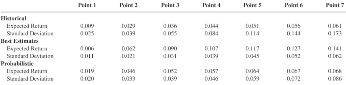
Table 1 and Figure 1 report expected returns for portfolios at different risk levels. The historical effi-cient frontier is estimated using Equation (1). We use returns over the past twenty-four weeks to calculate ex-pected returns and the variance-covariance matrix. The minimum-risk portfolio has a standard deviation of 2.5% and an expected return of 0.9%; the maxi-mum-risk portfolio has a standard deviation of 17.3% and an expected return of 6.1%.
We estimate the consensus best estimates efficient frontier by using Equation (8). We calculate the ex-pected returns and construct the variance-covariance
matrix using the market professionals’
one-week-ahead point and interval forecasts. The min-imum-risk portfolio has a standard deviation of 2.1% and an expected return of 0.4%; the maximum-risk portfolio has a standard deviation of 13.7% and an ex-pected return of 14.1%.
We estimate the consensus probabilistic efficient frontier by using Equation (11). We calculate expected returns and construct the variance-covariance matrix using the market professionals’ one-week-ahead probabilistic forecasts. The minimum-risk portfolio has a standard deviation of 2% and an expected return of 1.9%; the maximum-risk return portfolio has a stan-dard deviation of 8.6% and an expected return of 6.8%. The optimizer we use selects the risk levels for the minimum and maximum return portfolios given the raw data. We also calculate the expected return for a portfolio with a standard deviation of 3.9% for each ex-pectation formation process, based on historical data, point and interval forecasts, and probabilistic
fore-Table 1. Efficient Frontier Estimates
The historical efficient frontier is calculated by Markowitz optimization using the last twenty-four weekly returns of twenty-five high-volume ISE companies. Using Markowitz optimization, we calculate the consensus best estimates efficient frontier using professionals’
one-week-ahead point and interval price forecasts of twenty-five high-volume ISE companies. The professionals’ consensus probabilistic efficient frontier is calculated using Markowitz optimization, using their one-week-ahead probabilistic price forecasts of twenty-five high-volume ISE companies. Table columns report the seven data points along the efficient frontier. Point 1 is the minimum-risk portfolio, Point 7 is the maximum-risk portfolio, and other portfolios are selected evenly along the efficient frontier. The portfolio with a standard deviation of 0.0389 is the ISE 100 index tracking portfolio.
Point 1 Point 2 Point 3 Point 4 Point 5 Point 6 Point 7
Historical Expected Return 0.009 0.029 0.036 0.044 0.051 0.056 0.061 Standard Deviation 0.025 0.039 0.055 0.084 0.114 0.144 0.173 Best Estimates Expected Return 0.006 0.062 0.090 0.107 0.117 0.127 0.141 Standard Deviation 0.011 0.021 0.031 0.039 0.045 0.052 0.062 Probabilistic Expected Return 0.019 0.046 0.052 0.057 0.064 0.067 0.068 Standard Deviation 0.020 0.033 0.039 0.046 0.059 0.072 0.086 1 2 ( 6) ( 3) ( 6) (15) i i F CPFI F F CPFI - = - - - =
casts, respectively. This portfolio matches the histori-cal standard deviation of the index tracking portfolio. The expected return for this portfolio is 2.9% when past prices are the basis of the expectation formation process.
When we base our expectations on experts’ proba-bilistic forecasts, expected return increases to 5.2%. When we base our expectations on their point and in-terval estimates, expected return increases further to 5.8%. Similar rankings are depicted at all risk levels above 3.9%, which corresponds to the standard devia-tion of the index. At risk levels lower than the market risk, expected returns are highest when based on probabilistic forecasts.
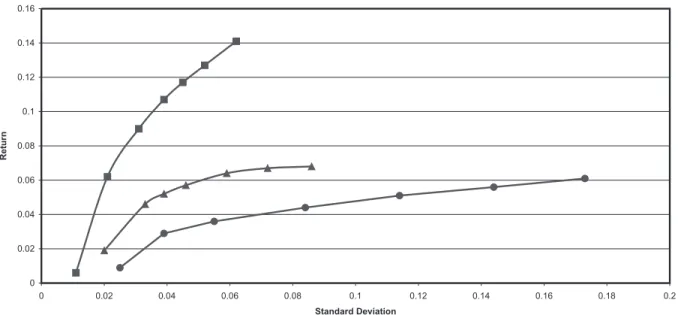
Figure 1 illustrates that expected returns are based on point and interval estimates at all risk levels except for the minimum-risk portfolio. Expected returns cal-culated using historical price series are the lowest at all risk levels. Expected returns based on probabilistic forecasts and point and interval forecasts are higher than those based on historical prices at all comparable risk levels. Expected returns based on point and inter-val forecasts are systematically higher than those based on probabilistic forecasts at all comparable risk levels, except again for the minimum-risk portfolio. Note here that the range of risk levels is largest for the historical efficient frontier, from a standard deviation of 2.5% to 13.7%, and smallest for the consensus best estimates frontier.
Table 1 and Figure 1 indicate that the consensus best estimates frontier, which is based on market profes-sionals’ point and interval forecasts, is the best in terms
of expected return per unit of risk at all risk levels. This may be misleading, however. Investors are concerned primarily with realized returns, not expected returns. It’s quite possible that realized returns will be consid-erably different from expected returns. Therefore, we next investigate the actual performance of the portfo-lios we have constructed so far, by comparing their re-alized returns with expected returns at all risk levels.
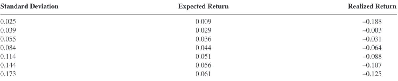
In Table 2 and Figure 2, we present realized versus expected returns at all risk levels for the historical effi-cient frontier. At all risk levels, realized returns are negative and well below expected returns. The mini-mum-risk portfolio (sd = 2.5%) realizes a huge loss of 18.8%, and the maximum-risk portfolio (sd = 17.3%) loses 12.5% in one week. The market tracking portfo-lio (sd = 3.9%) yields the minimum loss, 0.3%. Compared to expected returns that are positive at all risk levels, portfolios constructed using historical price data perform rather poorly.
For the minimum-risk portfolio, the discrepancy be-tween expected and realized returns is highest, 19.7%. This discrepancy is at a minimum for the market track-ing portfolio and increases systematically for portfo-lios with higher risk levels. For the maximum-risk portfolio, the discrepancy between expected and real-ized returns reaches 18.6%.
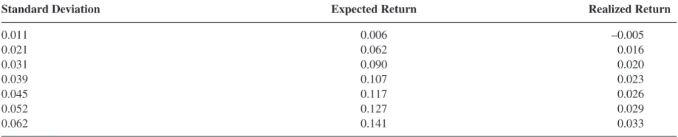
In Table 3 and Figure 3, we present realized versus expected returns at all risk levels for the best estimates efficient frontier. In this case, the expectation forma-tion process is based on experts’ point and interval forecasts. Realized returns are lower than expected re-turns at all risk levels, which is similar to what we
ob-FIGURE 1
served for the historical efficient frontier. However, this time, realized returns are positive at all risk levels except for the minimum-risk portfolio. The mini-mum-risk portfolio realizes a loss of 10.9%, with a standard deviation of 2.1%.
Realized returns increased consistently but gradu-ally as portfolio risk increased. The realized return for the maximum-risk portfolio (sd = 13.7%) reaches 3.3%. Realized returns are 11.3% lower than expected
returns for the minimum-risk portfolio (sd = 2.1%), 4.4% lower for the market tracking portfolio (sd = 3.9%), and 10.8% lower for the maximum-risk portfo-lio (sd = 13.7%).
Figure 4 and Table 4 report realized versus expected returns at all risk levels for the probabilistic efficient frontier. Similarly to what we found for the best esti-mate efficient frontier, realized returns are below ex-pected returns at all risk levels. At low-risk levels,
real-Table 2. Comparison of One-Week-Ahead Historical Efficient Frontier Portfolios and their Realized Returns
Column 1 reports the portfolios’ weekly standard deviations along the efficient frontier. Standard deviations are calculated from historical returns and the weight vectors obtained from the Markowitz optimization procedure using Equation (3). Column 2 reports the expected returns of the portfolios along the efficient frontier, which are calculated from historical returns and weight vectors obtained from the Markowitz optimization procedure using Equation (2). Column 3 calculates the realized returns for the portfolios using the weekly realized rates of returns following the estimation period and the weight vector obtained from the Markowitz optimization procedure using Equation (2). For example, the first row depicts the minimum-risk portfolio for the historical efficient frontier. Standard deviation is 0.025, expected return for the portfolio is 0.9%, and realized return the following week is –18.8%. The second row depicts the ISE 100 index tracking portfolio. Standard deviation is 0.039, expected return is 2.9%, and the realized return the following week is –0.3%.
Standard Deviation Expected Return Realized Return
0.025 0.009 –0.188 0.039 0.029 –0.003 0.055 0.036 –0.031 0.084 0.044 –0.064 0.114 0.051 –0.088 0.144 0.056 –0.107 0.173 0.061 –0.125 FIGURE 2
ized returns are negative, but improve consistently and become positive at high risk levels. The minimum-risk portfolio (sd = 2%) incurs a loss of 10.9%, making the discrepancy between expected and realized returns 12.8%. The realized return on the maximum-risk port-folio (sd = 8.6%) is 1.2%, still well below the expected return. The discrepancy between the two is 5.6%.
Figure 5 plots the realized returns from the three ef-ficient frontiers constructed on different expectation
formation processes using historical prices, point and interval forecasts, and probabilistic forecasts, respec-tively.
We find that if investors construct portfolios based on a standard expectation formation process that uses past price series, they would incur considerable losses. Moreover, the maximum loss, a huge 18.8%, would be realized for the minimum-risk portfolio, while the min-imum loss of 0.3% would be realized by the index
Table 3. Comparison of One-Week-Ahead Best Estimates Efficient Frontier Portfolios and their Realized Returns
Column 1 reports the weekly standard deviations of the portfolios along the consensus best estimates efficient frontier. Standard deviation for each stock is calculated from professionals’ consensus estimates by using Equation (12). Standard deviation for the portfolios is calculated using each stock’s standard deviation and the weight vector obtained from the Markowitz optimization procedure using Equation (3). Column 2 reports the expected returns of the portfolios along the best estimates efficient frontier. Expected returns for the portfolios are calculated from professionals’ consensus estimates using Equation (11) and the weight vector obtained from the Markowitz optimization procedure using Equation (2). Column 3 calculates the realized returns for the portfolios using the weekly realized rates of returns following the estimation period and the weight vector obtained from the Markowitz optimization procedure using Equation (2). For example, the first row is the minimum-risk portfolio for the consensus best estimates efficient frontier. Weekly standard deviation is 0.011, expected return is 0.6%, and realized return the following week is –0.5%. The fourth row depicts the ISE 100 index tracking portfolio. Standard deviation is 0.039, expected return is 10.7%, and realized return the following week is 2.3%.
Standard Deviation Expected Return Realized Return
0.011 0.006 –0.005 0.021 0.062 0.016 0.031 0.090 0.020 0.039 0.107 0.023 0.045 0.117 0.026 0.052 0.127 0.029 0.062 0.141 0.033 FIGURE 3
tracking portfolio. As portfolio risk increases, portfo-lio returns would deteriorate further, and the maxi-mum-risk portfolio would incur a loss of 12.5%.
If we invested in efficient portfolios constructed us-ing market professionals’ subjective expectations about stock prices, represented in the form of probabil-istic forecasts, we would improve portfolio perfor-mance at all comparable risk levels except for the
mar-ket tracking portfolio. We would incur milder losses at low risk levels and modest gains up to 1.2% at higher risk levels.
If we invested in efficient portfolios constructed us-ing market professionals’ subjective expectations about stock prices, represented in the form of point and interval forecasts, we would improve portfolio perfor-mance further at all comparable risk levels. In addition,
Table 4. Comparison of One-Week-Ahead Probabilistic Efficient Frontier Portfolios and their Realized Returns
Column 1 reports the weekly standard deviations of the portfolios along the consensus probabilistic efficient frontier. Standard deviation for each stock is calculated from professionals’ consensus probabilistic estimates by using Equation (15). Standard deviations for the portfolios are calculated using each stock’s standard deviation and the weight vector obtained from the Markowitz optimization procedure using Equation (3). Column 2 reports the expected returns of the portfolios along the probabilistic efficient frontier. Expected returns are calculated from professionals’ consensus probabilistic estimates using Equation (15) and the weight vector obtained from the Markowitz optimization procedure using Equation (2). Column 3 calculates the realized returns for the portfolios using the weekly realized rates of returns following the estimation period and the weight vector obtained from the Markowitz optimization procedure using Equation (2). For example, the first row depicts the minimum-risk portfolio for the consensus probabilistic efficient frontier. Weekly standard deviation is 0.020, expected return is 1.9%, and realized return the following week is –10.9%. The third row depicts the ISE 100 index tracking portfolio. Standard deviation is 0.039, expected return is 5.2%, and realized return the following week is –0.6%.
Standard Deviation Expected Return Realized Return
0.020 0.019 –0.109 0.033 0.046 –0.007 0.039 0.052 –0.006 0.046 0.057 –0.003 0.059 0.064 0.002 0.072 0.067 0.008 0.086 0.068 0.012 FIGURE 4
at all risk levels we would enjoy gains, except for the minimum-risk portfolio, which is still at a loss. In this case, portfolio performance improves considerably and systematically as the risk borne by the investor in-creases. It would be possible to earn weekly returns ranging from 1.4% to 3.3% using the best estimates ef-ficient frontier, which is clearly superior to returns from the probabilistic efficient frontier and the histori-cal efficient frontier at all risk levels.
Conclusions
This study has investigated two domains not cap-tured by previous research. First, we used expectation formation processes based on subjective forecasts in constructing the efficient frontier alternative. This choice helped us integrate human behavior into finan-cial modeling. We compared the performance of port-folios constructed using point, interval, and probabilis-tic forecasts to those constructed using the standard of time series data approach. We used actual portfolio managers as forecasters, and gave them a real-time, real-world assessment task. This increased ecological validity.
In a portfolio context, our results reveal that sub-jective forecasts, whether point, interval, or probabil-istic, perform better than the standard approach using past price series. The realized returns from portfolios constructed using subjective forecasts revealed a better understanding of the direction of market
move-ments. Investors were therefore better off construct-ing efficient portfolios based on subjective forecasts than using the standard Markowitz approach. Despite the immense literature on the poor forecast accuracy of subjective forecasts compared to econometric methods using past series, what counts is the actual portfolio performance of these forecasts. This is an example of better-performing financial models that use human judgment.
We expect further research in this field to investi-gate the expectation formation process. Possible biases in subjective forecasts must be explored so that the re-lated expected returns, expected standard deviations, and expected covariances can be calculated accord-ingly. For example, as long as the distributions given by forecasters are skewed, the point forecasts may rep-resent median rather than mean returns. Appropriate procedures must be developed and used to handle the
asymmetry in the dispersion. Dispersion and
comovements could be measured with metrics to cap-ture the biases in the forecast formation process. We hope that studies combining actual investor behavior and financial models will help us understand financial markets better and result in practitioners working with better models.
Acknowledgments
We would like to acknowledge the helpful com-ments of Werner DeBondt, Mezienne Lesfer and Roy
FIGURE 5
Batchelor on this and earlier versions of the paper. We would like to thank the anonymous fund managers who supplied the experimental data used in this study for their time and devotion.
Notes
1. TL = Turkish lira.
2. We thank Emre Berk for suggesting this procedure.
Reference
Andreassen, P.B. “Judgmental Extrapolation and Market Overreac-tion: On the Use and Disuse of News.” Journal of Behavioral
Decision Making, 3, (1990), pp. 153–174.
Basci, S., E. Basci, and G. Muradoglu. “Do Extreme Falls Help Fore-casting Stock.” CUBS Faculty of Finance Working Papers, No. 06, 2001.
De Bondt, W.F.M. “Betting on Trends: Intuitive Forecasts of Finan-cial Risk and Return.” International Journal of Forecasting, 9, (1993), pp. 355–371.
Fildes, R. “Efficient Use of Information in the Formation of Subjec-tive Industry Forecasts.” Journal of Forecasting, 10, (1991), pp. 597–617.
Fildes, R. “The Evaluation of Extrapolative Forecasting Methods.”
International Journal of Forecasting, 8, (1992), pp. 108.
Ippolito, R.A. “Efficiency with Costly Information: A Study of Mu-tual Fund Performance, 1965–1984.” Quarterly Journal of
Eco-nomics, 104, (1989), pp. 1–23.
Markowitz, H.M. Portfolio Selection. New York: John J. Wiley & Sons, 1959.
Markowitz, H.M. Portfolio Selection: Efficient Diversification of
In-vestments, 2nd ed. Cambridge, MA: Blackwell Publishers,
1991.
Muradoglu, G., and D. Onkal. “An Exploratory Analysis of Portfolio Managers’ Probabilistic Forecasts of Stock Prices.” Journal of
Forecasting, 13, (1994), pp. 565–578.
Önkal, D., and G. Muradoglu. “Evaluating Probabilistic Forecasts of Stock Prices in a Developing Stock Market.” European Journal
of Operations Research, 74, (1994), pp. 350–358.
Selcuk, F. “Is There a Term Structure of Interest Rates in Turkey?” Paper presented at the EEA meeting, New York, March 1995. Yates, J.F., L.S. McDaniel, and E.S. Brown. “Probabilistic Forecasts
of Stock Prices and Earnings: The Hazards of Nascent Exper-tise.” Organizational Behavior and Human Decision