Square root central difference-based FastSLAM approach improved by differential evolution

c

⃝ T¨UB˙ITAK

doi:10.3906/elk-1307-55 h t t p : / / j o u r n a l s . t u b i t a k . g o v . t r / e l e k t r i k /

Research Article

Square root central difference-based FastSLAM approach improved by differential

evolution

Haydar ANKIS¸HAN1,∗, Fikret ARI2, Emre ¨Oner TARTAN1, Ahmet G¨ung¨or PAKF˙IL˙IZ2

1

Department of Biomedical Equipment Technology, Vocational School of Technology, Ba¸skent University, Ankara, Turkey

2

Department of Electrical and Electronics Engineering, Faculty of Engineering, Ankara University, Ankara, Turkey

Received: 09.07.2013 • Accepted/Published Online: 29.01.2014 • Final Version: 23.03.2016

Abstract: This study presents a new approach to improve the performance of FastSLAM. The aim of the study is to

obtain a more robust algorithm for FastSLAM applications by using a Kalman filter that uses Stirling’s polynomial interpolation formula. In this paper, some new improvements have been proposed; the first approach is the square root central difference Kalman filter-based FastSLAM, called SRCD-FastSLAM. In this method, autonomous vehicle (or robot) position, landmarks’ position estimations, and importance weight calculations of the particle filter are provided by the SRCD-Kalman filter. The second approach is an improved version of the SRCD-FastSLAM in which particles are improved by a differential evolution (DE) algorithm for reducing the risk of the particle depletion problem. Simulation results are given as a comparison of FastSLAM II, unscented (U)-FastSLAM, SRCD-Kalman filter-aided FastSLAM, SRCD particle filter-based FastSLAM, FastSLAM, and DE-FastSLAM. The results show that SRCD-based FastSLAM approaches accurately compute mean and precise uncertainty of the robot position in comparison with FastSLAM II and U-FastSLAM methods. However, the best results are obtained by DE-SRCD-FastSLAM, which provides significantly more accurate and robust estimation with the help of DE with fewer particles. Moreover, consistency of the DE-SRCD-FastSLAM is more prolonged than that of FastSLAM II, U-FastSLAM, and SRCD-FastSLAM.

Key words: Simultaneous localization and mapping, square root central difference Kalman filter, Stirling’s polynomial

interpolation, differential evolution

1. Introduction

SLAM is a method for building a map of unknown environment using the position data of a robot or an autonomous vehicle in simultaneous processes [1,2]. In SLAM applications, classical methods generally use Kalman filter (KF)-based applications. However, a particle filter and its variants have been recently proposed for the solution of the SLAM problem [3–10].

FastSLAM applications are well-known methods as a solution for the SLAM problem [3–6]. FastSLAM can present the desired performance for large-scale map calculations in real-time applications due to its parallelized structure. Variations of FastSLAM methods are as follows: FastSLAM I, FastSLAM II, and U-FastSLAM

and improved versions that have previously been applied in the literature [3–10]. Some of them estimate

paths of vehicles by using Rao-Blackwellized particle filters [11] and positions of the features (landmarks) by ∗_{Correspondence: hankishan@baskent.edu.tr}

using an extended KF (EKF) or unscented KF (UKF). Besides their good performances, FastSLAM methods can also be used in non-Gaussian environments in real-time applications [3–6]. One of the most important abilities of the FastSLAM methods is the accurate estimation of uncertainty. Additionally, this algorithm gives information about the entire path history of the vehicle and its associated map. Another advantage of the FastSLAM algorithm is the success of data association, which is carried out by the advantage of the sampling distribution of each particle [12]. Each particle can have different numbers of feature (landmark) observations. In this algorithm, a novel approach is implemented for solving decision problems and is associated with different particles for different features. This is one of the characteristics of FastSLAM, which is the motivation of interest in multiple-hypothesis problems [12]. This has some advantages: vehicle motion noise does not affect the data association. If the data association is accurate for a particle and the other particles are incorrect, then incorrect particles have lower probabilities and they are removed in the next step [12]. Thus, the method eliminates incorrect associations.

There are some problems in FastSLAM applications. One of them is the degeneration problem, which is also a particle filter problem where weights of particles converge to zero in the resampling stages. Consequently, this phenomenon results in degeneration in EKF-based FastSLAM [13–15]. Another problem in EKF-FastSLAM is computational complexity of particles due to the number of particles. Selecting a large number of particles causes long computation time, and moreover the results converge to the real position of the robot or autonomous vehicle. On the contrary, in the case of using an insufficient number of particles, the performance is not good as desired.

In previous studies, unscented transformation (UT)-based filter approaches have been proposed for the

solution of the linearization problem of EKF-FastSLAM approaches [5,6]. These studies have shown that

the degeneration problem can be solved by using the UKF in the position estimation of vehicles and maps of the features (landmarks). Moreover, it was claimed in [6] that UKF-based FastSLAM can also solve the computational complexity of particle filter. However, there are some drawbacks in UKF-based (U)-FastSLAM, as follows:

- Adjusting three scaling parameters for calculating optimal sigma points is required at filter initialization. - Computational complexity of the particle filter is still a problem in U-FastSLAM that is needed to be

improved by any optimization algorithm.

- Covariance matrix is required to be positive semidefinite in each time step.

- Additional time is required due to the square root calculation of the covariance matrix.

There are some Kalman-based filters that can solve these kinds of problems in the literature. One of them is central difference-based Kalman filters (CDKFs). Square root central difference SR-CDKF shares some similarities with the UKF algorithm, such as pointwise evaluation of nonlinearities and weighted sum calculation. However, SR-CDKF has one important property different from the UKF algorithm. SR-CDKF uses Stirling’s polynomial interpolation formula to approximate the Bayesian integrals, whereas the UKF uses scaled unscented transformation (SUT) [16]. It was shown in [17] that SR-CDKF guarantees the positive semidefiniteness of the state covariance matrix. Moreover, instead of taking the square root of state covariance in the UKF, state covariance will be propagated directly in the SR-CDKF, which avoids the need to refactorize in each time step [18]. Additionally, SR-CDKF has a good advantage over UKF such that SR-CDKF is more adaptive than UKF [19]. In Gaussian distributions, the optimal value of scalar scaling parameters should be appropriately

selected in the UKF for different applications. However, SR-CDKF has only one scaling parameter, h , which

is equal to √3 for all Gaussian random variables. One study [20] used SR-CDKF in the SLAM problem with

the SR-unscented Kalman filter (SR-UKF)-based model. The results showed that SR-CDKF could be a good alternative to address the SLAM problem.

There are some naturally inspired optimization algorithms available for reducing the computational complexity of the particle filter in the literature [21–23]. One of them is the differential evolution (DE) algorithm. DE is a simple and efficient evolutionary optimization algorithm introduced by Storn and Price [24]. In the last decade, DE has been applied in a wide range of optimization problems [24–26] and its superiority has been proven in comparative studies. In this study, unlike previous ones, SRCD-based FastSLAM and its improved version (DE-improved SRCD-FastSLAM) have been used for the SLAM problem. It is able to reduce the computational complexity of particle filters using a minimum number of particles. In the sampling stage, particles can be moved from the low likelihood region to the high likelihood region with the help of DE. It is seen that DE not only improves particles, but also improves the computational efficiency of the SRCD-FastSLAM, and thus is able to obtain more robust results and less mean square error (MSE) than in previous studies.

2. Background of FastSLAM

Before the definition of the FastSLAM algorithm, we should explain the SLAM problem. It can be defined as simultaneous estimation of the vehicle position and building of the map of its observable environment. Recently, particle filters have been proposed for the solution of this problem [3–10]. In applications, joint probability

distribution p(xt_{, Θ|z}t_{, u}t_{, n}t_{) of the model is estimated for the path of the vehicle x}t_{= x}

1, ..., xt and posterior

density of feature maps Θ . The path of the vehicle and map of the environment at time t are calculated using information of the previous state and knowledge of control information at time t – 1 [3,4].

Feature-based mapping methods in SLAM assume that there are N features (landmarks) at t by Θ , and then the posterior is shown as

p(xt, Θ|zt, ut, nt), (1)

where nt= n1, ..., nt represents data association between features and measurement information, zt= z2, ..., zt

is the observation sequence, and ut= u1, ..., ut is the control input. In probabilistic perspective, a nonlinear

motion model for computing the posterior can be given as

p(xt|xt−1, ut), (2)

where xt represents current position, ut is control, and xt−1 is the previous position of the vehicle. However,

the measurement model owing to the probabilistic perspective is given as

p(zt|xt−1, Θ, nt). (3)

In FastSLAM applications, the state of the model is estimated in two stages as the path of the vehicle and the features map. This process is carried out by using a Rao-Blackwellized particle filter [11]. Posterior distribution is given as p(xt_{, Θ|z}t_{, u}t_{, n}t_{) = p(x}t_|zt_{, u}t_{, n}t₎ K ∏ k=1 p(θk|xt, zt, ut, nt), (4)

where θk represents the k th feature at time t . Each particle builds its own map at a particular time. The map

building process is done by parallel EKF in FastSLAM I and II and UKF in U-FastSLAM. Each particle forms the following:

X_ti= < xt,i, µi_1,t, Σi_1,t, ..., µi_N,t, Σi_N,t>, (5)

where i is the particle index xt,i_{, and µ}i

1,t, Σi1,t represent state and mean and covariance of the model,

respectively. In the method, the new position is estimated from the last motion model as given in Eq. (6).

xi_t∼ p(xtxit−1, ut) (6)

Not all FastSLAM approaches use the importance distribution computation and current measurement informa-tion. For example, FastSLAM I computes the posterior distribution by only using the motion model informainforma-tion. However, this approach results in some errors, since the model assumes that observation model noise informa-tion is known, which is not true in practical applicainforma-tions. To solve this problem the FastSLAM II method was proposed in [4]. This approach converges to the new position using both instant measurement and the motion

model, and the new position is given in Eq. (7).

xit∼ p(xtxt−1,i, ut, zt, nt) (7)

In unscented (U)-FastSLAM and FastSLAM II, importance sampling is given as follows.

w_ti= target distribution proposal distribution = p(xt,i_|zt_{, u}t_{, n}t p(xt−1,i|zt−1_{, u}t−1_{, n}t−1_)p(xi t|xt−1,i, zt, ut, nt) (8)

For details on the importance sampling derivation, the reader is referred to [4] and [6].

The map of the environment can be shown as a Gaussian distribution set in FastSLAM, so there is no need to calculate linear and quadratic computations in FastSLAM approaches. It was shown in [4] that this process reduces the computational complexity from M x N to M xlog N . However, this model has some drawbacks despite the improvements. In FastSLAM I and II (EKF-based FastSLAM) applications, due to the linearization, particle weights converge to zero in the resampling stage of the vehicle and feature position estimations, resulting in degeneration problems. Other studies [5,6] overcame this drawback by using SUT in FastSLAM II. In the U-FastSLAM approach, unlike FastSLAM I and II, the unscented Kalman filter (UKF) is used for computing vehicle position estimation, feature (landmark) position estimation, and importance weight calculation.

3. Proposed FastSLAM approach and computational complexity

There are some available studies related to the modified FastSLAM in the literature [3–10]. However, these approaches have some drawbacks. In this study, alternative improved FastSLAM approaches are proposed to overcome these drawbacks. Using the proposed methods to achieve better estimation accuracy and less computation time is the aim.

3.1. DE-based SRCD-FastSLAM

In this study, the proposed approaches perform computations in three stages as in FastSLAM II and U-FastSLAM: 1) vehicle state estimation, 2) feature state estimation, and 3) importance weight calculation.

3.1.1. Vehicle state estimation

Importance weight estimation has a significant role in Rao-Blackwellized particle filters. To achieve the proposal distribution it is required to obtain a correct a posteriori distribution. If the proposal distribution is greater than the statistical distribution, convergence of the proposal to the correct distribution may not be appropriate. There are some studies available in the literature [4,6,12,13] that used heuristic techniques to improve the accuracy of the proposal distribution. One such study [4] proposed the use of EKF-based FastSLAM approaches for the SLAM solutions. It was observed that the degeneration problem of particles in FastSLAM I and II occurred. In [6], the UKF-based FastSLAM approach was used for the solution of the SLAM problem. Instead of linearization, the U-FastSLAM method estimates sigma points using a deterministic approach to compute more accurate means and correct uncertainty of the vehicle. However, SRCD-FastSLAM, similar to U-FastSLAM, uses Stirling’s polynomial formula to calculate sigma points deterministically and propagate these points into the nonlinear function, so it computes a more correct mean and more precise uncertainty of the vehicle (see the Appendix) [19].

Because observations need not be taken in each time step in SLAM, proposal distribution and the vehicle position can occur in two steps: prediction and update steps.

3.1.1.1. SR-CDKF prediction stage

The vehicle state augmented vector and augmented covariance matrix are calculated by using control input and the observation, which are given as

xa,i_t−1 = [ xi_t−1 0 0 ]T = [ xi x,t₋₁ xiy,t₋₁ xiϕ,t−1 0 0 ]T , P_ta,i₋₁ =   P i t₋₁ 0 0 0 Qt 0 0 0 Rt   , (9)

where xa,i_t−1 is the augmented state and xi

t−1 is the state of the i th particle. In SR-CDKF, sigma points are

calculated with the help of the scaling parameter ( h) . This symmetrical set of 2 N + 1 sigma points χa(k),i_t−1 ,

which is similar to the SUT, for the vehicle augmented state vector can be calculated as χa(0),i_t−1 = xa,i_t−1

χa(k),i_t−1 = xa,i_t−1+ (hS_ta,i₋₁)k (k = 1, ..., N )

χa(k),i_t−1 = xa,i_t−1− (hS_ta,i₋₁)k (k = N + 1, ..., 2N )

, (10)

where k represents the k th column of a matrix. In SR-CDKF, each sigma point χa(k),i_t−1 has state, control, and

measurement components, which are given by χa(k),i_t−1 =

[

χ(k),i_t−1 χu(k),i_t χz(k),i_t

]T

. (11)

These sigma points are the same as SUT propagates through to a nonlinear function ( f ) with control information and added noise information.

¯ χ(k),i_t = f (ui t+ χ u(k),i t , χ (k),i t−1) = [ ¯

χ(k),i_x,t χ¯(k),i_y,t χ¯(k),i_φ,t

]T

In SR-CDKF, Stirling’s polynomial interpolation method estimates the posterior mean, covariance, and cross-covariance of vehicles and weighted regression of transformed sigma points, which are given as in [19]:

xi t/t₋₁ = 2N ∑ k=0 w(k)g χ¯(k),it S_t/t−₋₁ = qr         √ w(k)c1 ( ¯χ (k),i t,1:N− ¯χ (k),i t,N +1:2N) √ w(k)c2 ( ¯χ (k),i t,1:N+ ¯χ (k),i t,N +1:2N− 2¯χ (k),i t,0 )         (13)

where weight w(k)g is used to compute the posterior mean, and the other weight w(k)ci is used to compute

covariance and cross-covariance. These weights are calculated as shown below. w(0)g = h 2_−L h , w (k) g = _2h1 w(k)c1 = 1 4h2 , w (k) c2 = h2₋₁ 4h2 , k = 1, ..., 2N (14) 3.1.1.2. SR-CDKF update stage

Sigma points are calculated in the measurement update stage.

χa(k),i_t = [xa(k),i_t , xa(k),i_t ± (hS_ta(k),i₋₁ )k]

¯

χ(k),it = χ

(k),i

t

(15)

If the measurement information is available in SLAM applications, data association will be required to update vehicle state, covariance, and cross-covariance for each feature. The measurement equation is given as shown below. ¯ Z_t(k),i = h( ¯χ(k),i_t , µi ˆ m,t₋₁) + ¯χ z(k),i t ˆ zi t = 2N ∑ k=0 w(k)g Z¯t(k),i (16)

Here, µi_{m,tˆ −1} is the m th previous feature mean, and ˆzti is the predicted measurement. In SR-CDKF,

measure-ment update equations are given as in [18,19].

S_z,t− = qr         √ w(k)c1 ( ¯Z (k),i t,1:N− ¯Z (k),i t,N +1:2N) √ w(k)c2 ( ¯Z (k),i t,1:N− ¯Z (k),i t,N +1:2N− 2 ¯Z (k),i t,0 )         Σxtzt = √ w(k)c1 S − t/t₋₁ [ ¯ Z_t,1:N(k),i − ¯Z_{t,N +1:2N}(k),i ]T (17) K_ti = (Σxtzt/(S − z,t) T_)/S− z,t xit = xit/t−1+ K i t(zt− ˆzit) U = K_tiS_z,t− Si t = cholupdate{Sz,t−, U,−1} (18)

Here, Sz,t− represents innovation covariance and Kti represents Kalman gain. xit and Sti represent the estimated

mean and its covariance at time t , respectively. The mean and its covariance generate a Gaussian for each particle, and the mean is sampled as

xi_t∼ N(xi_t, S_ti). (19)

If there is no feature information, the vehicle state is estimated from the available measurement. However, if

there is feature information, the measurement update equations (Eqs. (16)–(18)) are repeated for each observed

feature. The sigma point χa(k),it is refreshed by Eq. (13).

3.1.2. Feature state estimation

There are some SLAM applications available in the literature that use CDKF [17,19,20]. These studies use CDKF for feature estimations as described in the following subsections.

3.1.2.1. Feature update stage

In FastSLAM applications, the feature update stage defines the sigma points that use the previously registered mean and feature covariance. In the proposed algorithm, sigma points’ calculation and covariance estimation for each feature are given as follows.

χ(0),i _{= µ}i Lt,t−1 χ(k),i = µi_L t,t−1+ (hP i Lt,t−1) , (k = 1, ..., L) χ(k),i _{= µ}i Lt,t−1− (hP i Lt,t−1) , (k = L + 1, ..., 2L) (20)

Here, L is the state dimension ( L = 2 for the landmarks), χ(k),i _{represents sigma points of features, i is the}

index of the i th particle, and Pi

Lt,t−1is a 2 × 2 feature covariance matrix. The weights of features are given in

Eq. (14). Measurement update equations for the features are also given as

¯ Z_t(k),i = h(χ(k),i_{, x}i t) , k = 0, 1, ..., 2L ˆ zi t = 2N ∑ k=0 wg(k)Z¯ (k),i t , (21)

where ˆzti represents the predicted measurement and h (.) is the nonlinear observation model, and ¯Z

(k),i

t is

the transformed sigma points. Owing to Eq. (21), Kalman gain, cross-covariance, and innovation covariance

matrices are calculated as follows.

S_y,t− = qr            √ w(k)c1 (χ (k),i t,1:N− χ (k),i t,N +1:2N)∗ √ w(k)c2 (χ (k),i t,1:N+ χ (k),i t,N +1:2N− 2χ (k),i t,0 )            Pxtyt = 2L ∑ k=0 wc(k)[χ(k),i− µiLt,t−1][χ (k),i_{− µ}i Lt,t−1] T Ki t = (Pxtyt/(S − y,t)T)/Sy,t− (22)

Finally, updated feature mean µi_Lt,t and its covariance P_Li_t,t of the i th particle are calculated. µi_Lt,t = µi_Lt,t−1+ Kti(zt− ˆzti) V = Ki tSy,t− Pi Lt,t = cholupdate{S − y,t, V,−1} (23)

Here, zt is the true measurement. Each feature is updated by Cholesky factorization. As a result of using

this method, the algorithm becomes more stable. Moreover, because of sigma point calculation increasing the computational complexity of model, the SRCD-based model does not calculate the square root of the covariance matrix for each time step directly using it, so some processing time is saved. Feature initialization has an important role in SLAM applications. This process is realized with the available measurement information and noise covariance.

3.1.2.2. Feature initialization stage

In the SRCD-FastSLAM approach, the feature initialization algorithms for each particle is given as follows.

ϕ(0),i _{= z} t ϕ(k),i _{= z} t+ (h √ Rt), (k = 0, ..., L) ϕ(k),i _{= z} t− (h √ Rt), (k = L + 1, ..., 2L) (24) M_t(k),i = h−1(ϕ(k),i_{, ˆχ}i t) , (k = 0, ..., 2L) µi Lt,t = 2L ∑ k=0 w(k)g Mt(k),i Pi Lt,t = qr {[√ w(k)c (M (k),i t − µiLt,t) √ Rt ]} P_Li_t,t = cholupdate { P_Li_t,t, Mt(0),i− µiLt,t, w (0) c } (25)

3.1.3. Calculation of importance weight and resampling

Importance weights corresponding to the last observation are calculated as follows:

Wti = 2πBti −(1/2) exp { −(1/2)(zt− ˆzti )T( Bti )−1( zt− ˆzti )} , (26) where Bi t = ( P_tx,L,i )T( Si t )₋₁ P_tx,L,i+ Si

y,t . The effective numbers of particles in the resampling stage are

calculated as follows:

Tef f = ∑M 1

i=1( ˆWi)2 , (27)

where M is the total number of particles and ˆWi _{is the normalized i th particle. When T}

ef f decreases below

3.2. SRCD-FastSLAM improved by DE

Optimization algorithms are recently used for moving particles from the low likelihood to the high likelihood region in particle filters. In this study, DE, which is a well-known optimization algorithm, was chosen because the DE algorithm has some advantages compared with particle swarm optimization (PSO) and the genetic algorithm (GA). For instance, a small number of parameters need to be set. The algorithm is based on the difference in the population, and so it obtains diversity and converges to the best results. Another advantage of the algorithm is that it has a more robust convergence property to true values than PSO [26]. In comparative studies, it is shown that DE has a more suitable convergence property [25,26]. It is thought that this kind of positive advantages will provide good results for the DE-based FastSLAM model in SLAM applications. The algorithm works in an iterative way in SLAM. The DE algorithm is given in four steps:

Initialization: Like the other population-based algorithms, DE starts with distributing the population

into the search space, which has a predefined size Np. In DE, the population at the g th iteration, Pg, consists

of Np target vectors represented as xg,iwhere i is the vector index. In the first generation target vectors are

initialized as

xj,i,0 = bj,l+ randj[0, 1).(bj,u− bj,l) , (28)

where j = 1,2, . . . ,D represents the dimension number of the vector.

Mutation: To diversify the population, DE uses two operators: mutation and crossover. The mutation operator simplifies the used vector differences to obtain a mutant vector. DE varies according to the used base vector in mutation operation. Variants of DE are represented as DE/x/y/z, where x denotes the base vector, y denotes the number of difference vectors used, and z represents the crossover method. In the classic variant of DE, represented as DE/rand/1/bin, the mutant vector is obtained as

vi,g = xr0,g+ F.(xr1,g− xr2,g) , (29)

where r0, r1, and r2 are randomly chosen distinct indexes and different from target index i . The scale factor,

F ∈ (0, 1+), is a positive number generally selected smaller than 1. In this study we use the best vector as the base vector that yields a faster convergence generally. The mutant vector is then given as

vi,g = xbest,g+ F.(xr1,g− xr2,g) . (30)

Crossover: In crossover, the mutant vector is used to be recombined with the target vector by the crossover operator, which mixes the parameters of two vectors as

ui,g = uj,i,g

{

vj,i,g, if(randj[0, 1)≤ Cr or j = jrand)

xj,i,g otherwise

, (31)

where ui,g is the trial vector .

Selection: Finally, in the selection process, the objective function value of the trial vector is simply compared with the target vectors and the best vector is kept as the target vector for the next generation. This

cycle is repeated for all Np vectors and the updated target population becomes ready for the next one at the

A fitness function must be defined for the particle’s optimization. The recommended fitness function is: Fitness = exp { − 1 2Rvt (zt,new− ˆzit,pred) 2 } , (32) where Rv

t represents vehicle measurement noise variance, zt,new the last obtained measurement, and ˆzt,predi the

estimated measurement. With the help of the calculated fitness function, all particles will move to the optimal particle position. Two scaling parameters that are used for adjusting DE include the mutation scaling factor.

In this study, it is chosen as F = 0.4, and crossover probability is chosen as Cr = 0.8. These values, which are

adjusted optimal values, were obtained from different Cr and F values in the simulations. Updated particles

depending on the fitness function during sampling of particles are reused in the distribution. The optimization process of particles is carried out in the sampling stage of the particle filter.

3.3. Computational complexity of the DE-SRCD-FastSLAM

In this section, the proposed models will be compared with the U-FastSLAM and FastSLAM II methods. As is known, weight importance may converge to zero in time steps, leading to degeneration of particles. Moreover, another important problem is the computational complexity of the particle filter, which causes a negative impact on the system processing time. U-FastSLAM eliminates the degeneration problem of EKF-based FastSLAM approaches [6]. U-FastSLAM is sigma point KF-based SLAM approach. Without linearization, UKF-based SLAM uses a deterministic approach to estimate sigma points from probability, and these points propagate to the nonlinear function. The degeneration problem that is encountered in EKF-based FastSLAM can be solved with this model. However, state error covariance must be positive semidefinite and the calculation time of sigma points is another problem in UKF-based FastSLAM. The time for FastSLAM approaches is O(MN ) with features in FastSLAM I, FastSLAM II, and U-FastSLAM. The SRCD-FastSLAM approach needs less time than FastSLAM II and U-FastSLAM for simulation because the improved version of SRCD-FastSLAM uses a minimum number of particles in simulations. Its results show that while using fewer particles it can provide results as efficient as those of U-FastSLAM and FastSLAM II. In the simulation results, it will be shown that the minimum numbers of particles are selected. The flowchart for the DE-improved SRCD-based FastSLAM approach is given in Figure 1.

4. Results and discussion

Simulation results were carried out in four stages: in the first application, the FastSLAM II, U-FastSLAM, SRCD-Aided FastSLAM, SRCD particle filter-based FastSLAM, and SRCD-FastSLAM methods were compared. In the first simulation, data association was assumed to be known. In the second simulation, U-FastSLAM, SRCD-FastSLAM, and DE-improved (DE)-SRCD-FastSLAM approaches were compared with the new scenario. In this simulation, data association was assumed to be unknown, and the nearest neighbor method was used for the data association problem. The third simulation was examined to calculate filter consistencies for the SLAM problem. The DE-SRCD-FastSLAM results were compared with the U-FastSLAM and FastSLAM II approaches. The data association was assumed to be known for this simulation. The last simulation was applied to the Victoria Park dataset that is an outdoor SLAM application. The results were compared with FastSLAM II, U-FastSLAM, and SRCD-FastSLAM.

SRCD – DE – FastSLAM (z u Xt, ,t t1,Q Rt, t):

L= feature dimension; N= vehicle dimension

Sigma point parameter

Calculate sigma point weights ( ( )k

g

w , ( )k c

w , k=0,…,2L (2N))

A. Initialization Step

a. Particle velocity, position, fitness function b. Initialize first generation target vectors of DE

For all particles

Retrieve X_{t 1}

Predict mean and covariance of the vehicle (13) For all observations

ˆ

k= Compatibility test

End For

For kˆ = known feature

B. Move particles using DE from low likelihood region to high likelihood region that minimizes fitness function

a. Adjust the particles’ best local position with the best fitness value as the global best

b. Updating swarm, According to (20), velocity of particle is calculated and vehicle position is updated (17-18)

c. Process returns to B, pbest and lbest are updated

d. At the end of iteration go e. Refresh sigma points C. Computation of importance weight

a. Calculate importance weight (26)

b. Draw the sample from proposal distribution (19) c. Weight calculation

End For

If kˆ= new feature

Calculate new feature mean and covariance (25) Repeat B and C

Else

Update mean and covariance of feature (22-23)

End if Add ( ) ( ), , , , , , k k i t t i_{L t L t}Pi t t x μ to X_aux End For D. Resampling

Figure 1. Pseudocode of the SRCD-based FastSLAM improved by DE.

4.1. Simulation I

Bailey et al. [1] developed a SLAM simulator and opened it to all SLAM researchers. The different SLAM algorithms can be easily compared with this simulator. Moreover, [1] showed the consistency of the FastSLAM II with this simulator. As the simulator allows the comparison of different algorithms, we chose to use this software. In this simulation, selected parameters are given as vehicle speed of 3 m/s, wheelbase of 4 m, and control frequency of 40 Hz. However, control and observation noise variances are given as:

Q = [ 1.02 ₀ 0 [10× (π/180)]2 ] , (33)

R = [ 1.22 ₀ 0 [12× (π/180)]2 ] . (34)

Observation parameters are maximum laser range of 30 m and vehicle scanning frequency between observations of 5 Hz. In this simulation, data association is assumed to be known. Related scenario results are given in Figure 2, and obtained estimation results are given in Figure 3.

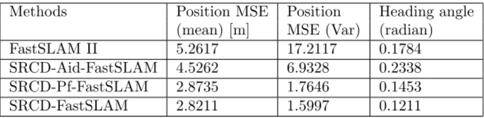
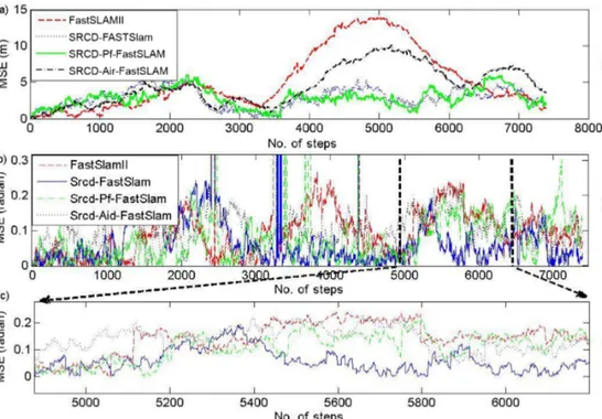
Simulation results have shown that the FastSLAM II approach has the greatest MSE between 3500 and 6000 time steps. It is observed that the position MSE of the vehicle is quite high in comparison with other proposed methods. The reason for this great error is thought to be the fact that the Kalman-based filter (EKF) badly affects the FastSLAM model. Figure 3 and 4 show that the best estimation results are obtained by SRCD-FastSLAM. MSE results of the position and heading angles are given in Table 1.

–100 –50 0 50 –40 –20 0 20 40 x (m) y (m) –100 –80 –60 –40 –20 0 20 40 60 80 –40 –20 0 20 40 x (m) y (m ) (c) (a) –100 –50 0 50 –40 –20 0 20 40 x (m) y (m) –100 –80 –60 –40 –20 0 20 40 60 80 –40 –20 0 20 40 x (m) y (m ) (d) (b)

Figure 2. Estimated and true vehicle paths with estimated and true landmarks. a) FastSLAM II, b) SRCD-Aided

FastSLAM, c) SRCD-Particle Filter Based FastSLAM, d) SRCD-FastSLAM. Green line and blue stars denote the true path and landmarks, respectively. The blue line is the estimated mean of the vehicle position and red dots are estimated landmarks.

Table 1. Average mean square error (MSE) results for Simulation I.

Methods Position MSE Position Heading angle

(mean) [m] MSE (Var) (radian)

FastSLAM II 5.2617 17.2117 0.1784

SRCD-Aid-FastSLAM 4.5262 6.9328 0.2338

SRCD-Pf-FastSLAM 2.8735 1.7646 0.1453

Figure 3. Mean square errors (MSEs) of the methods: a) position errors (m), b) heading angle errors (rad), c) magnified

details of the heading angle errors.

0 2 4 6 8 10 12 14 4 3 2 1

1−FastSLAM II, 2−SRCD−Aid−FastSLAM, 3−SRCD−Pf−FastSLAM, 4− SRCD−FastSLAM

MSE (m)

Figure 4. Boxplot drawing of the algorithms: 1) FastSLAM II, 2) SRCD-Aid-FastSLAM, 3) SRCD-Pf-FastSLAM, and

4) SRCD-FastSLAM.

FastSLAM II results are compared with other methods that have higher MSEs than the SRCD-based FastSLAM approaches. In FastSLAM II, vehicle position, feature position, and importance weights estimations were calculated by EKF. Due to the linearization in the EKF, FastSLAM II has some drawbacks such as risk of particle depletion overtime and the vehicle state mean divergence. Thus, an undesired mapping will be created. The proposed SR-CDKF-based approaches provide feasible results that can be seen in Figure 3. However, there is an important detail in Figures 2 and 3. The SRCD particle filter-based FastSLAM and SRCD-FastSLAM approaches’ results are very close to each other. Despite SRCD-aided FastSLAM results being better than those of FastSLAM II, they are fairly lower than those of the other proposed SRCD-based FastSLAM approaches. It is seen that path estimations of the vehicle are better than position estimations of the features in the SRCD-based

FastSLAM approaches. The results of heading angle errors show that SRCD-aided FastSLAM has the largest MSE. Boxplot drawings of MSE values obtained by different SLAM algorithms are given in Figure 4.

4.2. Simulation II: performance comparison of U-FastSLAM and SRCD-based FastSLAM

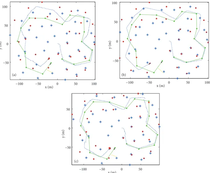
In this simulation, it is assumed that the data association is unknown and the nearest neighbor method is used for the association. DE-SRCD-FastSLAM results are compared with SRCD-FastSLAM and U-FastSLAM. A scenario was created by making use of the software developed in [1]. The chosen particle number for the U-FastSLAM and SRCD-FastSLAM methods is 30; however, for DE-SRCD-FastSLAM it is 3. The system and observation parameters have been adjusted similar to Simulation I and the knowledge of control and

measurement noise is the same as in Simulation I. DE algorithm crossover probability ( Cr) is 0.8 and mutation

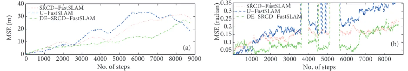
scale factor ( F ) is 0.4. The results are given in Figure 5, MSE results are given in Figure 6, and numeric values of the MSE of position and heading angles are given in Table 2.

−100 −50 0 50 100 −50 0 50 100 x (m) y (m) −100 −50 0 50 −50 0 50 x (m) y (m) −100 −50 0 50 100 −50 0 50 100 x (m) y (m) (a) (b) (c)

Figure 5. Estimated and true vehicle paths with the landmarks. a) U-FastSLAM, b) SRCD-FastSLAM, c)

DE-SRCD-FastSLAM. Here, green lines and blue stars denote the true path and landmarks, respectively. The blue lines represent the estimated mean of the vehicle position and red dots are estimated landmarks.

Table 2. Average mean square error (MSE) results for Simulation II.

Methods U-FastSLAM SRCD-FastSLAM DE-SRCD-FastSLAM

Position MSE (mean, m) 18.4513 16.5021 11.2039

Position MSE (Var) 120.0046 95.3682 42.8834

Heading Angle (rad) 0.5669 0.5156 0.4157

It is seen that the most suitable results are obtained by DE-SRCD-FastSLAM in Figure 6 because DE improves each particle and moves particles from the low to the high likelihood region. This leads to improvement in the performance of the approach, so in terms of MSE better results are obtained for the path of the vehicle. In Figure 6, the MSE and variance values have grown at the about same rate for SRCD-FastSLAM and U-FastSLAM methods. However, DE-SRCD-U-FastSLAM position MSE and heading angle errors are lower than in the other methods and they do not grow in parallel with them.

0 1000 2000 3000 4000 5000 6000 7000 8000 9000 0 10 20 30 40 No. of steps MSE (m) SRCD−FastSLAM U−FastSLAM DE−SRCD−FastSLAM 1000 2000 3000 4000 5000 6000 7000 8000 0.05 0.1 0.15 0.2 0.25 0.3 0.35 No. of steps MSE (rad

ian) SRCD−FastSLAMU−FastSLAM DE−SRCD−FastSLAM

(b) (a)

Figure 6. Mean square errors (MSEs) of U-FastSLAM, SRCD-FastSLAM, and DE-SRCD-FastSLAM: a) position errors

(m), b) heading angle errors (rad).

As seen in the simulation the SRCD-based FastSLAM performances are good in comparison with both EKF- and UKF-based FastSLAM approaches. The first advantage of the methods is to solve the depletion problem of particles. In addition, the computational complexity of particle filters could be reduced by using a minimum number of particles with the help of DE. It is shown in Table 2 that U-FastSLAM must calculate the square root of the covariance matrices for the requirement of being positive semidefinite, and scaling parameters such as α , β , and λ must be adjusted depending on the Gaussian distribution at filter initialization. However, SRCD-based FastSLAM approaches only used one scaling parameter ( h) . The optimal h parameter is equal to the kurtosis values of the a priori random variable. Although Kim et al. [5,6] said that U-FastSLAM reduced the computational complexity of FastSLAM in comparison with EKF-based FastSLAM approaches, we can see that U-FastSLAM is still insufficient to solve these problems, and it needs to be improved by using an optimization algorithm. For this reason, in this study, we have used DE for optimization of particles.

4.3. Simulation III: evaluation of DE-SRCD-FastSLAM consistency

In this section we try to evaluate the filters’ consistency depending on the average normalized estimation error squared (NEES) being used as a measure. We performed thirty Monte Carlo simulations for each filter with the two-sided 95% probability region. The related acceptance interval was between 2.19 and 3.93.

Vehicle wheelbase was set as 0.26 m with 0.8 m/s vehicle velocity. The control frequency was 40 Hz and

sensor frequency was 5 Hz. Control noises were 0.4 m/s in velocity and 4◦ in steering angle, and measurement

noises were 0.2 m/s in range and 2◦ in bearing. The maximum sensor range was 5 m, with 180◦ frontal field

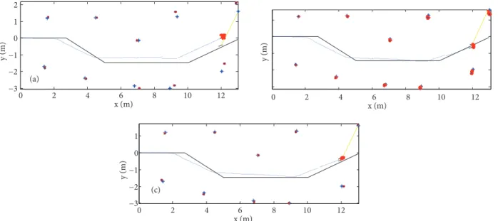
0 2 4 6 8 10 12 −3 −2 −1 0 1 2 x (m) y (m) y (m) (a) 0 2 4 6 8 10 12 −3 −2 −1 0 1 x (m) 0 2 4 6 8 10 12 x (m) y (m) (c)

Figure 7. Estimated and true vehicle paths with the landmarks: a) FastSLAM II, b) U-FastSLAM, and c)

DE-SRCD-FastSLAM. The black lines represent the true path, and blue asterisks represent true landmark positions. The blue line and red asterisks represent estimated mean of the vehicle and landmarks positions, respectively. These cases were used for 100 particles for FastSLAM II and U-FastSLAM and 10 particles for DE-SRCD-FastSLAM.

100 200 300 400 500 600

0 2 4

FastSLAMII NEES results

No. of steps A. NEES ove r 30 M.C.R. 100 200 300 400 500 600 0 1 2 3 4

U−FastSLAM NEES results

No. of steps A. N E E S ov er 30 M.C.R. 100 200 300 400 500 600 0 1 2 3 4

DE−SRCD−FastSLAM NEES results

No. of steps A. NE E S ove r 30 M. C.R. (a) (b) (c)

Figure 8. Consistency of a) FastSLAM II with 100 particles, b) U-FastSLAM with 100 particles, and c)

DE-SRCD-FastSLAM with 10 particles. M.C.R. = Monte Carlo runs.

Figure 7 gives all estimation results of the methods. It is seen from Figure 7 that the best results are obtained by DE-SRCD-FastSLAM. With the help of DE particle distribution is improved, and consequently minimum variances are obtained in landmarks and the estimated vehicle path becomes the closest one to the true path. In other words, the desired accuracy is obtained due to the particles’ correct distribution around the posterior.

As seen in Figure 8, the best results are again obtained by DE-SRCD-FastSLAM. DE-SRCD-FastSLAM maintains consistency in the required interval and its result is more prolonged than the FastSLAM II and

U-FastSLAM approaches’ results. In this simulation, DE-SRCD-U-FastSLAM used 10 particles; however, U-FastSLAM II and U-FastSLAM used 100 particles.

4.4. Simulation IV: outdoor SLAM application

In this simulation, an outdoor SLAM application is carried out. The SRCD-FastSLAM method was compared to FastSLAM II and U-FastSLAM using the Sydney Victoria Park dataset, which is a popular dataset in the SLAM community. A Victoria Park image with GPS data represented by an intermittent yellow line is given in Figure 9.

The used vehicle information is a wheelbase of 2.83 m equipped with the SICK laser range finder with

a 180◦ frontal FOV. The velocity and the steering angle were obtained by encoders. While measuring the

information, some undesired errors occurred due to wheel slippage and vehicle movement. Therefore, the

odometry information coming from the encoder is poor.

We thank Guivant and Nedot [27] for generating the Victoria Park dataset. In the park, although

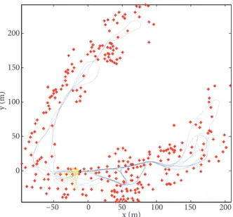
the vehicle was equipped with GPS, the sensor gave intermittent information owing to the limited satellite information. However, ground true position of the vehicle was enough to estimate the vehicle state of the filter. Estimation results of the SRCD-FastSLAM algorithm with 3 particles is given in Figure 10, and comparative estimation results of FastSLAM II, U-FastSLAM, and SRCD-FastSLAM algorithms are given in Figure 11.

−50 0 50 100 150 200 0 50 100 150 200 x (m) y (m)

Figure 9. Victoria Park, Sydney, Australia, with GPS

data.

Figure 10. Victoria Park, Sydney, Australia. SRCD-FastSLAM-based estimation results for vehicle path (blue line) and estimated landmarks (red asterisks) with 3 par-ticles.

It is seen that the performance of SRCD-FastSLAM with 3 particles is better than the results of the other approaches. The best estimated path result, which is compatible with the GPS data, was obtained by SRCD-FastSLAM. Since the used SR-CDKF provides better estimation results compared with others with GPS data, the uncertainties are propagated well and the accuracy of the vehicle state estimation has been improved with the proposed method. As seen, the U-FastSLAM result being better than that of FastSLAM II is owing to the used unscented-based Kalman filter.

Figure 11. Victoria park estimation results of a) FastSLAM II with 3 particles, b) U-FastSLAM with 3 particles, and

c) SRCD-FastSLAM with 3 particles. In all figures, the thick green line denotes GPS data and the solid blue line is the estimated path. The red asterisks are the estimated positions of the landmark. The control noises in the simulation are σv = 0.4 m/s and σγ = 1.4◦, and measurement noises are σv= 0.5 m/s and συ = 1.5◦. In this simulation it is assumed that data association is unknown and nearest neighbor method was used with the 2 σ acceptance region.

5. Conclusions

In the literature, EKF- and UKF-based approaches are generally examined in FastSLAM applications. These ap-proaches have some drawbacks, such as EKF-based apap-proaches leading to the particles undergoing degeneration over time. This problem may lead to some undesired results in the case of building the map of the environment and obtaining vehicle position. In addition, the computational complexity of EKF-based FastSLAM is another problem. However, it is clear in the literature that UKF-based approaches can also solve the degeneration problem, but the sigma point calculation of the UKF-based FastSLAM increases the computational complexity

and the a posteriori covariance matrix needs to be positive semidefinite. The tuning of the scaling parameters, which are important for calculation of sigma points, is the other difficulty. SRCD-based approaches use only one scaling parameter ( h) for estimating the sigma points in Gaussian distribution. Moreover, SRCD-based FastSLAM approaches are also able to solve the degeneration problem. Simulation results show that the desired method improves the vehicle position estimation and the building of the map of the environment according to the previous methods. The other contribution of the proposed method is the reduced computational complexity of the covariance matrix, which is directly calculated in the SRCD-based FastSLAM. Simulation results show that the best performances in terms of both the position and the heading angle errors are obtained by the DE-SRCD-FastSLAM approach.

References

[1] Durrant-Whyte H, Bailey T. Simultaneous localization and mapping: Part I. IEEE Robot Autom Mag 2006; 2: 99–108.

[2] Bailey T, Durrant-Whyte H. Simultaneous localization and mapping: Part II. IEEE Robot Autom Mag 2006; 3: 108–117.

[3] Montemerlo M, Thrun S, Koller D, Wegbreit B. FastSLAM: A factored solution to the simultaneous localization and mapping problem. In: Proceedings of the Eighteenth National Conference on Artificial Intelligence; 2002; Menlo Park, CA, USA. Palo Alto, CA, USA: AAAI. pp. 593–598.

[4] Montemerlo M, Thrun S, Koller D, Wegbreit B. FastSLAM2.0: An improved particle ?ltering algorithm for simultaneous localization and mapping that provably converges. In: Proceedings of the 18th International Joint Conference on Artificial Intelligence; 2003; Acapulco, Mexico. pp. 1151–1156.

[5] Kim C, Sakthivel R, Chung WK. Unscented FastSLAM: A robust algorithm for simultaneous localization and mapping problem. In: Proceedings of the IEEE International Conference on Robotics & Automation; 2007; Rome, Italy. New York, NY, USA: IEEE. pp. 2439–2445.

[6] Kim C, Sakthivel R, Chung WK. Unscented FastSLAM: a robust and efficient solution to the SLAM problem. IEEE T Robot 2008; 24: 808–820.

[7] Havangi R, Teshnehlab M, Nekoui MA. A neuro-fuzzy multi swarm FastSLAM framework. Journal of Computing 2010; 3: 83–94.

[8] Song Y, Li Q, Kang Y, Yan D. Square root cubature FastSLAM algorithm for mobile robot simultaneous localization and mapping. In: International Conference on Mechatronics and Automation; 5–8 August 2012; Chengdu, China. New York, NY, USA: IEEE. pp. 1162–1167.

[9] Wang X, Zhang H. A UPF-UKF framework for SLAM. In: Proceedings of the IEEE International Conference on Robotics and Automation; 2007; Rome, Italy. New York, NY, USA: IEEE. pp. 1664–1669.

[10] Dongbo L, Guorong L, Miaohua Y. An improved FastSLAM framework based on particle swarm optimization and unscented particle filter. Journal of Computational Information Systems 2012; 7: 2859–2866.

[11] Murphy K. Bayesian map learning in dynamic environments. In: NIPS Proceedings; 1999; Cambridge, MA, USA. pp. 1015–1021.

[12] Montemerlo M, Thrun S. Simultaneous localization and mapping with unknown data association using FastSLAM. In: IEEE International Conference on Robotics and Automation; 2003; Piscataway, NJ, USA. New York, NY, USA: IEEE. pp. 1985–1991.

[13] Bailey T, Nieto J, Nebot E. Consistency of the FastSLAM algorithm. In: Proceedings of the IEEE International Conference on Robotics and Automation; 2006; Orlando, FL, USA. New York, NY, USA: IEEE. pp. 424–429.

[14] Bailey T, Nieto J, Guivant J, Stevens M, Nebot E. Consistency of the EKF-SLAM algorithm. In Proceedings of the IEEE/RSJ International Conference of Intelligent Robots Systems; 2006; Beijing, China. New York, NY, USA: IEEE. pp. 3562–3568.

[15] Huang S, Dissanayake G. Convergence and consistency analysis for extended Kalman filter based SLAM. IEEE T Robot 2007; 5: 1036–1049.

[16] Julier S. The scaled unscented transformation. In: Proceedings of the American Control Conference; 2002. New York, NY, USA: IEEE. pp. 4555–4559.

[17] Norgaard M, Poulsen N, Ravn O. New developments in state estimation for nonlinear systems. Automatica 2000; 36; 1627–1638.

[18] Van Der Merwe R. Sigma-point Kalman filters for probabilistic inference in dynamic state-space models. PhD, OGI School of Science & Engineering at Oregon Health & Science University, Portland, OR, USA, 2004.

[19] Zhu J, Zheng N, Yuan Z, Zhang Q, Zhang X, He Y. A SLAM algorithm based on central difference Kalman filter. In: 2009 IEEE Intelligent Vehicle Symposium; 2009; Xi’an, China. New York, NY, USA: IEEE. pp. 123–128.

[20] Ankı¸shan H, Efe M. E¸szamanlı konum belirleme ve harita olu¸sturmaya Kalman filter yakla¸sımları. Dicle ¨Universitesi M¨uhendislik Fak¨ultesi Dergisi 2010; 1: 13–20.

[21] Ji C, Zhang Y, Tong M, Yang S. Particle filter with swarm move for optimization. Lect Notes Comp Sci 2008; 5199: 909–918.

[22] Yanan W, Jie C, Minggang G. Improved differential evolution-based particle filter algorithm for target tracking. In: 30th Chinese Control Conference; 2011; Yantai, China. New York, NY, USA: IEEE. pp. 3009–3014.

[23] Kwok NM, Fang G, Zhou W. Evolutionary particle filter: re-sampling from the genetic algorithm perspective. In: 2005 IEEE/RSJ International Conference on Intelligent Robots and Systems; 2005. New York, NY, USA: IEEE. pp. 2935–2940.

[24] Storn R, Price K. Differential Evolution – A Simple and Efficient Adaptive Scheme for Global Optimization over Continuous Spaces. Technical Report TR-95-012. Berkeley, CA, USA: International Computer Science Institute, 1995.

[25] Das S, Suganthan PN. Differential evolution: a survey of the state-of-the-art. IEEE T Evolut Comput 2011; 15: 4–31.

[26] Vesterstrom J, Thomsen R. A comparative study of differential evolution, particle swarm optimization, and evo-lutionary algorithms on numerical benchmark problems. In: Congress on Evoevo-lutionary Computation; 2004. New York, NY, USA: IEEE. pp. 1980–1987.

[27] Guivant J, Nedot E. Simultaneous Localization and Map Building: Test Case for Outdoor Applications. Sydney, Australia: Australian Centre for Field Robotics, Department of Mechanical and Mechatronic Engineering, The University of Sydney, Australia, 2006.

Appendix

A. Motion model due to the sigma points

In this study, for explaining the motion model, we introduce an easily understandable notation. Each state of the k th sigma points is formed in three components as follows:

χk,i_t−1 =    χk,i_x,t−1 χk,i_y,t−1 χk,i_φ,t−1    . (35)

Due to the Ackerman model, the control inputs [ Vt, Gt]T can be shown in the additive control noise component

χu(k),i_t [5,6]: [ Vn Gn ] = [ Vt + χu(k),i_V,t Gt + χu(k),i_G,t ] , (36) Where χu(k),i_t = [ χu(k),i_V,t χu(k),i_G,t ] . (37)

In this study, sigma point components are propagated through the Ackerman model, which is as follows:

¯ χk,i_t = χk,i_t−1 +   Vn ∆t cos( Gn + χ k,i φ,t−1 ) Vn ∆t cos( Gn + χk,iφ,t−1 ) Vn ∆t (sin(Gn)/wheelbase)   . (38)

B. Feature update augmentation

In the feature update stage of the SRCD-FastSLAM application, the augmented state of the feature is updated by using the previous feature mean and its covariance [5,6]:

µa,i_L t,t−1= [ µi Lt,t−1 0 ] , Σa,i_L t,t−1= [ Σi Lt,t−1 0 0 Rt ] (39) where µi

Lt,t−1 represents the mean of the L th feature, Σ

i

Lt,t−1 represents its covariance matrix, and Rt

represents the measurement noise covariance.

In the SRCD-based FastSLAM, sigma points are calculated by using these augmented states and Kalman

gain ¯Ki

t, which is calculated by Eq. (22). While calculating the Kalman gain, Rt is not used in the innovation