c
⃝ T¨UB˙ITAK
doi:10.3906/elk-1112-26 h t t p : / / j o u r n a l s . t u b i t a k . g o v . t r / e l e k t r i k /
Research Article
Shifted-modified Chebyshev filters
Metin S¸ENG ¨UL∗Faculty of Engineering and Natural Sciences, Kadir Has University, Cibali, Fatih, ˙Istanbul, Turkey
Received: 07.12.2011 • Accepted: 17.04.2012 • Published Online: 12.08.2013 • Printed: 06.09.2013
Abstract: This paper introduces a new type of filter approximation method that utilizes shifted-modified Chebyshev
filters. Construction of the new filters involves the use of shifted-modified Chebyshev polynomials that are formed using the roots of conventional Chebyshev polynomials. The study also includes 2 tables containing the shifted-modified Chebyshev polynomials and the normalized element values for the low-pass prototype filters up to degree 6. The transducer power gain, group delay, and impulse and step responses of the proposed filters are compared with those of the Butterworth and Chebyshev filters, and a sixth-order filter design example is presented to illustrate the implementation of the new method.
Key words: Butterworth filters, Chebyshev filters, filters, network
1. Introduction
There are numerous types of filters and design procedures [1–13], and in the design of low-pass filters, the amplitude approximation to the ideal normalized amplitude response is the most commonly used method. The ideal normalized amplitude response can be described as follows:
|H(jω)|2
= 1,|ω| < 1
= 0,|ω| > 1. (1)
This expression can be approximated by the following amplitude function:
|H(jω)|2
= 1
1 + ε2P2
n(ω)
, (2)
where n is the filter order, Pn(ω) is a polynomial of degree n , and ε is a filter parameter.
If a filter has a maximally flat amplitude characteristic, then it is referred to as a Butterworth filter, for which Pn(ω) = ω2n. However, if a filter has the maximum possible attenuation for the given variation in the
pass-band for the amplitude function, then Pn(ω) = Tn2(ω) , where Tn(ω) is the Chebyshev polynomial of degree
n [14]. If a linear phase response is desired, a Bessel filter is known to be the best choice [15]. In this case, Pn(ω) is based on the Bessel polynomials of degree n . If the greatest possible cutoff rate for the monotonically
decreasing amplitude is desired, then L -filters must be used [16]. For L -filters, Pn(ω) = Ln(ω2) , where Ln(x)
is a polynomial of degree n obtained from a linear combination of Legendre polynomials.
None of the filters mentioned above provide strong results in terms of the amplitude, phase, impulse and step responses. In choosing a filter, these 4 responses must be taken into consideration. For example, the Chebyshev filter has poor phase, impulse, and step responses, but has a good amplitude response. On the other hand, the Bessel filter is not suitable as a low-pass filter, but its phase response is optimum. The phase response of the Butterworth filter is better than that of the Chebyshev filter, and the amplitude response is better than that of the Bessel filter. On the other hand, the Chebyshev amplitude response and the Bessel phase response are much better than those of the Butterworth filter [17].
For equiripple pass-band and maximally flat stop-band response, Chebyshev filters are used. They have very sharp insertion loss characteristics around the cutoff frequency and the Chebyshev approximation has the lowest complexity and the steepest cutoff outside of the pass-band. No other polynomial has these optimum properties [18]. As a result, it is still the most common amplitude approximation used by filter designers, although the Butterworth approximation is much simpler mathematically.
The proposed filters can be considered as a new kind of transitional Butterworth–Chebyshev filter [19,20], since the properties lie between those of the conventional Butterworth and Chebyshev filters, as can be seen in Section 3. The poles of a transitional Butterworth–Chebyshev filter are a mixture of the poles of the conventional Butterworth and Chebyshev filters. However, in our approach, we utilize a new polynomial set, which is based on the roots of the conventional Chebyshev polynomials for chained-function filters [21]. This approach can result in various transfer functions having the same order, but different steady-state and transient characteristics. This filter type has practical advantages in rectangular waveguide and microstrip technologies [21–23].
The next section first explains the rationales for the proposed approach. After providing tables that present shifted-modified Chebyshev polynomials and element values for low-pass shifted-modified Chebyshev filter prototypes up to degree 6, this section draws comparisons between the transducer power gain, group delay, and impulse and step responses of the proposed filters with those of the Butterworth and Chebyshev filters. This section also describes a model for a prototype filter.
2. Rationales of the new approach
The proposed filter type can be considered as a compromise between the Butterworth and Chebyshev approxi-mations.
In the proposed approach, the polynomial Pn(ω) in Eq. (2) is formed using the roots of lower-order
conventional Chebyshev polynomials. For instance, to be able to obtain a polynomial of degree 6, the roots of the conventional Chebyshev polynomial of degree 3 can be used with a multiplicity of 2. Clearly there are numerous possibilities to obtain a new polynomial of degree 6, and naturally all of these polynomials have conventional Chebyshev polynomial roots. The mathematical details can be found in [21].
For instance, let us form a polynomial of degree 6 using the roots of the conventional Chebyshev polynomial of degree 3, which is T3(ω) = 4 ω3− 3 ω , with a multiplicity of 2. The roots of this polynomial
are 0, 0.866, and –0.866. If these roots are used, the following polynomial of degree 6 is obtained: Pm,6(ω) =
ω6− 1.5 ω4+ 0.5625 ω2 (which is the fourth modified Chebyshev polynomial of degree 6 seen in Table 1). The conventional Chebyshev polynomial of degree 6 is T6(ω) = 32 ω6− 48 ω4+ 18 ω2− 1 [24].
3. Filter characteristics
There are several characteristics that describe a filter’s performance. The insertion loss and group-delay re-sponses are the most important steady-state frequency domain rere-sponses. Moreover, there are several important transient responses, such as the impulse and step responses.
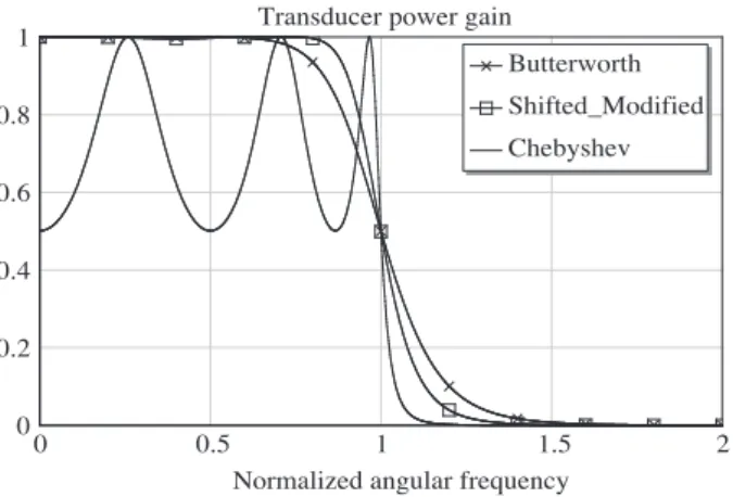
If the magnitude-squared frequency responses of the proposed filters are drawn, it is seen that at the cutoff frequency ( ω = 1) , |H(jω)|2̸= 0.5, while for the Chebyshev and Butterworth approximations, it is 0.5. An example can be seen in Figure 1 for n = 6 .
To be able to obtain a similar response, the coefficients of the polynomials formed via conventional Chebyshev polynomial roots must be scaled. A shifted-modified new polynomial set can be obtained by the substitution ω→ ω · ωx. Here, ωx is the frequency where the magnitude-squared frequency response is 0.5. For
the given example, using Eq. (2) with Pn(ω) = Pm,6(ω) , ω = 1 , and ε = 1 , ωxis 1.246 (see Figure 1), and then
the following shifted-modified polynomial is obtained: Ps−m,6(ω) = 3.7423 ω6− 3.6156 ω4+ 0.8733 ω2 (which
is the fourth shifted-modified Chebyshev polynomial of degree 6 seen in Table 1). If the magnitude-squared frequency response is drawn again, the curve seen in Figure 2 is obtained.
0 0.5 1 1.5 2
Normalized angular frequency Transducer power gain
0 0.2 0.4 0.6 0.8 1 Butterworth Modified Chebyshev 0 0.5 1 1.5 2
Normalized angular frequency Transducer power gain
0 0.2 0.4 0.6 0.8 1 Butterworth Shifted_Modified Chebyshev
Figure 1. Magnitude-squared frequency responses for a
sixth-order Butterworth, modified Chebyshev, and con-ventional Chebyshev filter.
Figure 2. Magnitude-squared frequency responses for a
sixth-order Butterworth, shifted-modified Chebyshev, and conventional Chebyshev filter.
It is clear from Figure 2 that the obtained filter response has no ripple in the pass-band and stop-band, as in Butterworth filter. It can be concluded that the magnitude-squared frequency response of the shifted-modified Chebyshev filter is better than that of the Butterworth (it is close to unity in a wider band in the pass-band) and the Chebyshev filter in the pass-band (there is no ripple in the pass-band). On the other hand, in the stop-band, it is better than that of the Butterworth filter, but worse than that of the Chebyshev filter. In the transition region, the Chebyshev filter has the sharpest response, and the proposed filter has a better transition response than that of the Butterworth filter.
As mentioned earlier, different n -order shifted-modified polynomials can be formed using lower-order conventional Chebyshev polynomial roots. Some of the combinations will give a quasi-equiripple pass-band response, while others will not. However, it should be mentioned that for all of the combinations, this ripple level is always less than or equal to that of the conventional Chebyshev approximation.
The pole locations of the transfer functions for a sixth-order Butterworth, shifted-modified Chebyshev, and conventional Chebyshev filter can be seen in Figure 3. The left-most poles, the right-most poles, and the middle poles belong to the Butterworth, conventional Chebyshev, and proposed filter, respectively.
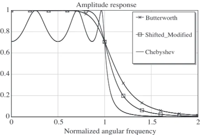
The amplitude and phase responses for a sixth-order Butterworth, shifted-modified Chebyshev, and conventional Chebyshev filter are given in Figures 4 and 5, respectively.
-1 -0.9 -0.8 -0.7 -0.6 -0.5 -0.4 -0.3 -0.2 -0.1 0 -1 -0.8 -0.6 -0.4 -0.2 0 0.2 0.4 0.6 0.8 1 Pole locations Real axis Im agi na ry a xi s 0 0.5 1 1.5 2
Normalized angular frequency Amplitude response 0 0.2 0.4 0.6 0.8 1 Butterworth Shifted_Modified Chebyshev
Figure 3. Pole locations for a sixth-order Butterworth,
shifted-modified Chebyshev, and conventional Chebyshev filter.
Figure 4. Amplitude responses for a sixth-order But-terworth, shifted-modified Chebyshev, and conventional Chebyshev filter.
As can be seen in Figures 4 and 5, the amplitude and phase response of the proposed filter is between those of the Butterworth filter and the conventional Chebyshev filter.
The group delay of the filters can be calculated by differentiating its phase response with respect to the angular frequency. It is known that the larger the ripple level of a conventional Chebyshev filter, the greater the group-delay around the cutoff frequency. As a result, signals with frequencies around the cutoff frequency stay within the filter for a longer duration, and naturally the output signal of the filter will be distorted.
The group-delay performance of the proposed filter is found between those of the Butterworth and conventional Chebyshev responses, as can be seen in Figure 6.
0 0.5 1 1.5 2
Normalized angular frequency Phase response (degrees)
-600 -500 -400 -300 -200 -100 0 Butterworth Shifted_Modified Chebyshev 0 0.5 1 1.5 2
Normalized angular frequency Group delay (s) 0 10 20 30 Butterworth Shifted_Modified Chebyshev
Figure 5. Phase responses for a sixth-order Butterworth,
shifted-modified Chebyshev, and conventional Chebyshev filter.
Figure 6. Group-delay responses for n = 6 .
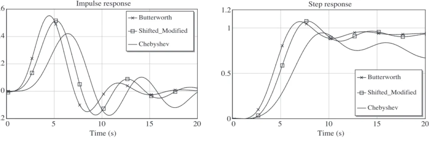
The impulse and step responses for a sixth-order conventional Chebyshev, a Butterworth, and the proposed filter can be seen in Figures 7 and 8, respectively.
Once again, the proposed filter responses are found between the Butterworth and conventional Chebyshev approximations.
0 5 10 15 20 Time (s) Impulse response -0.2 0 0.2 0.4 0.6 Butterworth Shifted_Modified Chebyshev 0 5 10 15 20 Time (s) Step response 0 0.5 1 1.2 Butterworth Shifted_Modified Chebyshev
Figure 7. Impulse responses for n = 6 . Figure 8. Step responses for n = 6 .
In Table 1, all of the possible modified and shifted-modified Chebyshev polynomials and frequency scaling factors ( ωx) are given from degrees 1 to 6.
Table 1. Modified and shifted-modified Chebyshev polynomials ( n = 1to6 ).
Degree (n) Modified Chebyshev polynomials ωx Shifted-modified Chebyshev polynomials
1 ω 1 ω 2 ω 2 1 ω2 ω2− 0.5 1.2247 1.5 ω2− 0.5 3 ω 3 1 ω3 ω3− 0.5 ω 1.1654 1.5828 ω3− 0.5827 ω 4 ω4 1 ω4 ω4− 0.75 ω2 1.2012 2.0819 ω4− 1.0822 ω2 ω4− 0.5 ω2 1.1317 1.6403 ω4− 0.6404 ω2 5 ω5 1 ω5 ω5− ω3+ 0.125 ω 1.2141 2.6380 ω5− 1.7896 ω3+ 0.1518 ω ω5− ω3+ 0.25 ω 1.1902 2.3884 ω5− 1.6860 ω3+ 0.2975 ω ω5+ 0.75 ω3 1.1714 2.2055 ω5− 1.2055 ω3 ω5− 0.5 ω3 1.1098 1.6834 ω5− 0.6834 ω3 ω5− 1.25 ω3+ 0.375 ω 1.2379 2.9069 ω5− 2.3712 ω3+ 0.4642 ω 6 ω6 1 ω6 ω6− 1.25 ω4+ 0.3125 ω2 1.2209 3.3111 ω6− 2.7769 ω4+ 0.4658 ω2 ω6− 1.5 ω4+ 0.625 ω2− 0.0625 1.2416 3.6640 ω6− 3.5650 ω4+ 0.9635 ω2− 0.0625 ω6− 1.5 ω4+ 0.5625 ω2 1.2460 3.7423 ω6− 3.6156 ω4+ 0.8733 ω2 ω6− ω4+ 0.125 ω2 1.1885 2.8189 ω6− 1.9955 ω4+ 0.1766 ω2 ω6− 0.75 ω4 1.1498 2.3109 ω6− 1.3110 ω4 ω6− 0.5 ω4 1.0943 1.7169 ω6− 0.7169 ω4 ω6− 1.5 ω4+ 0.75 ω2− 0.125 1.2247 3.3750 ω6− 3.3750 ω4+ 1.1250 ω2− 0.125 ω6− 1.25 ω4+ 0.375 ω2 1.2089 3.1221 ω6− 2.6702 ω4+ 0.5481 ω2 ω6− ω4+ 0.25 ω2 1.1654 2.5049 ω6− 1.8444 ω4+ 0.3395 ω2
For all of the degrees, the first possibility is formed using the root of the conventional Chebyshev polynomial of degree 1 with a multiplicity of n . For instance, the first possibility for n = 6 is Pm,6(ω) = ω6,
which is formed using the root of the conventional Chebyshev polynomial of degree 1 with a multiplicity of 6. As can be seen from Table 1, there is no modification for the first possibilities between the modified and shifted-modified Chebyshev polynomials ( ωx= 1) . It can also be noted that these first possibilities are the same
as the polynomials used for the Butterworth filters. Namely, it can be concluded that the polynomials used to obtain the Butterworth filters also have conventional Chebyshev polynomial roots; namely, the Butterworth polynomials of degree n have the root of the conventional Chebyshev polynomial of degree 1 with a multiplicity of n .
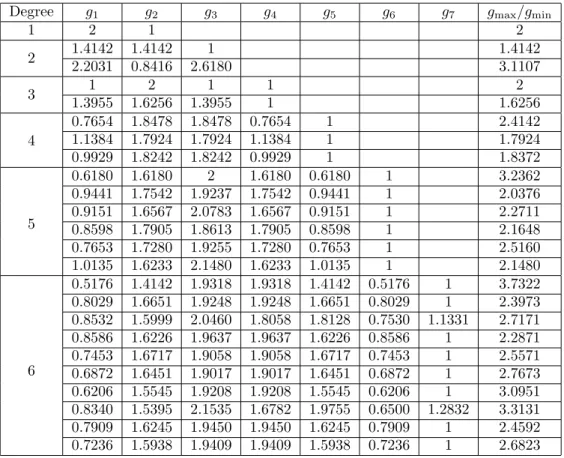
In Table 2, the element values for the low-pass inductor-capacitor (LC) ladder shifted-modified Chebyshev filter prototypes (3 dB ripple) are given from degrees 1 to 6, where g0 and ωc are the normalized source
resistance and normalized cut-off frequency, respectively. The first element ( g1) can be a series inductor or a
parallel capacitor.
Table 2. Element values for the low-pass LC ladder shifted-modified Chebyshev filter prototypes ( g0 = 1, ωc= 1, n = 1
to 6 3 dB ripple).
Degree g1 g2 g3 g4 g5 g6 g7 gmax/gmin
1 2 1 2 2 1.4142 1.4142 1 1.4142 2.2031 0.8416 2.6180 3.1107 3 1 2 1 1 2 1.3955 1.6256 1.3955 1 1.6256 4 0.7654 1.8478 1.8478 0.7654 1 2.4142 1.1384 1.7924 1.7924 1.1384 1 1.7924 0.9929 1.8242 1.8242 0.9929 1 1.8372 5 0.6180 1.6180 2 1.6180 0.6180 1 3.2362 0.9441 1.7542 1.9237 1.7542 0.9441 1 2.0376 0.9151 1.6567 2.0783 1.6567 0.9151 1 2.2711 0.8598 1.7905 1.8613 1.7905 0.8598 1 2.1648 0.7653 1.7280 1.9255 1.7280 0.7653 1 2.5160 1.0135 1.6233 2.1480 1.6233 1.0135 1 2.1480 6 0.5176 1.4142 1.9318 1.9318 1.4142 0.5176 1 3.7322 0.8029 1.6651 1.9248 1.9248 1.6651 0.8029 1 2.3973 0.8532 1.5999 2.0460 1.8058 1.8128 0.7530 1.1331 2.7171 0.8586 1.6226 1.9637 1.9637 1.6226 0.8586 1 2.2871 0.7453 1.6717 1.9058 1.9058 1.6717 0.7453 1 2.5571 0.6872 1.6451 1.9017 1.9017 1.6451 0.6872 1 2.7673 0.6206 1.5545 1.9208 1.9208 1.5545 0.6206 1 3.0951 0.8340 1.5395 2.1535 1.6782 1.9755 0.6500 1.2832 3.3131 0.7909 1.6245 1.9450 1.9450 1.6245 0.7909 1 2.4592 0.7236 1.5938 1.9409 1.9409 1.5938 0.7236 1 2.6823
For the conventional Chebyshev approximation, none of the elements of the even-order filters have the same value, i.e. they are asymmetric, but the odd-order approximations are symmetric. On the other hand, for the proposed filters, the even-order filters can be designed to be symmetrical if both of the terminations are equal. However, the conventional Chebyshev filters with even orders have unequal termination impedances.
ratio must be kept as small as possible. As can be seen from Table 2, different root combinations result in different gmax/gmin ratios.
4. Example
Here a sixth-order low-pass shifted-modified Chebyshev filter prototype will be designed using the element values given in Table 2, where it can be seen that 10 different sixth-order filter prototypes can be designed and 2 of them have different terminations.
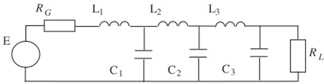
Figure 9 presents 1 of the possible low-pass shifted-modified Chebyshev filter prototypes of degree 6. Moreover, the element values for the Butterworth and conventional Chebyshev filter prototypes of degree 6 are given in Figure 9. The frequency and time domain characteristics of the filters are given in Section 3, in Figures 2 and 4–8. C2 C1 C3 L3 L R G R Ê L1 L2 E
Figure 9. The obtained proposed low-pass shifted-modified Chebyshev filter prototype: L1= C3= 0.8586, C1 = L3=
1.6226, L2= C2 = 1.9637, RG= RL= 1 ; Butterworth: L1 = C3= 0.5176, C1 = L3 = 1.4142, L2= C2 = 1.9318, RG=
RL= 1 ; and Chebyshev: L1= 3.5045, C1 = 0.7685, L2= 4.6061, C2= 0.7929, L3= 4.4641, C3= 0.6033, RG= 1, RL=
5.8095 .
The low-pass filter prototypes are normalized designs having a source impedance of RG= 1 and a cutoff
frequency of ωc = 1 . These designs must be scaled in terms of their impedance and frequency, and must
be converted to produce high-pass, band-pass, or band-stop characteristics. The details of the scaling and transformation can be found in [24].
5. Conclusion
In this paper, a new type of filter approximation method has been presented. Based on the conventional Chebyshev polynomial roots, new polynomials called modified Chebyshev polynomials have been defined, and then these polynomials have been shifted. These final polynomials are here referred to as shifted-modified Chebyshev polynomials, to be utilized for the designing of new types of filter prototypes.
This study has shown that these new filters have higher roll-off characteristics than Butterworth filters and a much lower ripple in the pass-band than conventional Chebyshev filters. In addition, they have impulse and step responses between those of the Butterworth and Chebyshev filters. Such shifted-modified Chebyshev filters can thus serve as a bridge between the Butterworth and conventional Chebyshev filters.
References
[1] B.A. Shenoi, Introduction to Digital Signal Processing and Filter Design, Hoboken, NJ, USA, Wiley, 2006. [2] D. Baez-Lopez, V. Jimenez-Fernandez, “Modified Chebyshev filter design”, Canadian Conference on Electrical and
Computer Engineering, Vol. 2, pp. 642–646, 2000.
[3] T. Zhi-hong, C. Qing-Xin, “Determining transmission zeros of general Chebyshev lowpass prototype filter”, Inter-national Conference on Microwave and Millimeter Wave Technology, pp. 1–4, 2007.
[5] A.V. Oppenheim, R.W. Schafer, Discrete-Time Signal Processing, 2nd ed., Upper Saddle River, NJ, USA, Prentice Hall, 1999.
[6] P.P. Vaidyanathan, Multirate Systems and Filter Banks, Upper Saddle River, NJ, USA, Prentice Hall, 1993. [7] N.K. Bose, Digital Filters: Theory and Application, New York, Elsevier, 1985.
[8] M.E. Van Valkenburg, Analog Filter Design, New York, Rinehart and Winston, 1982. [9] W.D. Stanley, Digital Signal Processing, Reston Publishing, Reston, VA, USA, 1975.
[10] M.F. Aburdene, T.J. Goodman, “The discrete Pascal transform and its applications”, IEEE Signal Processing Letters, Vol. 12, pp. 493–495, 2005.
[11] T.J. Goodman, M.F. Aburdene, “Pascal filters”, IEEE Transactions on Circuits and Systems I: Regular Papers, Vol. 55, pp. 3090–3094, 2008.
[12] H.G. Dimopoulos, “Optimal use of some classical approximations in filter design”, IEEE Transactions on Circuits and Systems II: Express Briefs, Vol. 54, pp. 780–784, 2007.
[13] U. C¸ am, S. ¨Olmez, “A novel square-root domain realization of first order all-pass filters”, Turkish Journal of Electrical Engineering & Computer Sciences, Vol. 18, pp. 141–146, 2010.
[14] P. Richards, “Universal optimum-response curves for arbitrarily coupled resonators” Proceedings of the IRE, Vol. 34, pp. 624–629, 1946.
[15] L. Storch, “Synthesis of constant-time delay ladder networks using Bessel polynomials”, Proceedings of the IRE, Vol. 42, pp. 1666–1675, 1954.
[16] A. Papoulis, “Optimum filters with monotonic response”, Proceedings of the IRE, Vol. 46, pp. 606–609, 1958. [17] D.E. Johnson, Introduction to Filter Theory, Upper Saddle River, NJ, USA, Prentice Hall, 1976.
[18] A.I. Zverev, Handbook of Filter Synthesis, New York, Wiley, 1967.
[19] A. Budak, P. Aronhime, “Transitional Butterworth–Chebyshev filters”, IEEE Transactions on Circuit Theory, Vol. 18, pp. 413–415, 1971.
[20] C.S. Gargour, V. Ramachandran, “A simple design method for transitional Butterworth-Chebyshev filters”, Journal of the Institution of Electronic and Radio Engineers, Vol. 58, pp. 291–294, 1988.
[21] C.E. Chrisostomidis, S. Lucyszyn, “On the theory of chained-function filters”, IEEE Transactions on Microwave Theory and Techniques, Vol. 53, pp. 3142–3151, 2005.
[22] M. Guglielmi, G. Connor, “Chained function filters”, IEEE Microwave and Guided Wave Letters, Vol. 7, pp. 390–392, 1997.
[23] C.E. Chrisostomidis, M. Guglielmi, P. Young, S. Lucyszyn, “Application of chained functions to low-cost microwave bandpass filters using standard PCB etching techniques” 30th European Microwave Conference, pp. 1–4, 2000. [24] D.M. Pozar, Microwave Engineering, 3rd ed., Hoboken, NJ, USA, Wiley, 2005.