FORECASTING EXCHANGE RATES USING
ARTIFICIAL NEURAL NETWORKS
BELMA DEN Z ONARAN
105664016
STANBUL B LG ÜN VERS TES
SOSYAL B L MLER ENST TÜSÜ
ULUSLARARASI F NANS YÜKSEK L SANS PROGRAMI
PROF. DR. AHMET SÜERDEM
2010
ii
Forecasting Exchange Rates Using Artificial Neural Networks
Yapay Sinir A ları ile Döviz Kuru Tahmini
Belma Deniz Onaran
105664016
Prof. Dr. Ahmet Süerdem :
Prof. Dr. Oral Erdo an :
Ö r.Gör. Kenan Tata :
Tezin Onaylandı ı Tarih: : 22.03.2010
Toplam Sayfa Sayısı:58
Anahtar Kelimeler (Türkçe)
Anahtar Kelimeler ( ngilizce)
1) Yapay sinir a ları
1) Artificial Neural Networks
2) Döviz kurları
2) Exchange Rates
3) Tahmin
3) Forecasting
4) Do rusal olmayan sistemler
4) Non-linear systems
ABSTRACT
The foreign exchange market is one of the largest and most volatile of the financial markets.
As the world globalized, the movement of exchange rates started to affect almost every individual and it became very critical to conjecture the route of the rates.
But foreign exchange rates are affected by many highly correlated economical, political and even psychological factors, and it is therefore very difficult to forecast the changes in exchange rate movements.
In this thesis, artificial neural networks is chosen in order to forecast the exchange rates. The reasons for choosing this model are explained, and a model is built to forecast the USD/TRY rate.
As the neural networks can be used to model both linear and non-linear relationships in data, and can approximate complex functional relationships, it was an accurate tool to work with.
ii
ÖZET
Döviz piyasası, finansal piyasalar arasındaki en büyük ve en de i ken piyasalardan biridir.
Küreselle meyle birlikte döviz kuru hareketleri neredeyse her bireyi etkilemeye ba ladı ve kur hareketlerinin tahmini çok daha kirtik bir hale geldi.
Ancak kur hareketleri birçok yüksek korelasyonlu ekonomik, politik ve hatta psikolojik faktörden etkilenir ve bu nedenle de tahmin edilebilmesi çok zordur.
Bu tezde döviz kuru hareketlerinin modellemesi ve tahmini için yapay sinir a ları kullanılacaktır. Yapay sinir a larının neden seçildi i açıklanacak, ve USD/TRY paritesinin tahmini için bir model olu turulacaktır.
Yapay sinir a ları, hem do rusal hem de do rusal olmayan sistemleri modellemede kullanılabilmesi ve karma ık problemleri çözebilme yetene i nedeniyle bu çalı ma için oldukça uygun bir metod olu turmu tur.
iii
ACKNOWLEDGEMENTS
I would like to express my sincere gratitude and appreciation to my supervisor Prof. Dr. Ahmet Süerdem for his assistance and guidance throughout the preparation of this thesis, and to Prof. Dr. Oral Erdogan for his valuable contributions.
iv
TABLE OF CONTENTS
1. INTRODUCTION...1
2. OVERVIEW OF NEURAL NETWORKS ...2
2.1 What is a Neural Network ...2
2.2 Historical Background ...4
2.3 A Simple Neuron ...5
3. ARCHITECTURE OF NEURAL NETWORKS ...6
3.1 Feed-forward networks ...6
3.1.1 The Back propagation Algorithm...8
3.2 Feedback Networks...9
3.3 Perceptrons...10
4. FORECASTING APPLICATIONS OF NEURAL NETWORKS...11
4.1 Literature Review ...12
5. COMPLEXITY, CHAOS AND NON LINEARITY ...15
5.1. Complexity...15
5.2.Chaos Theory...15
5.3. Linearity and Non-linearity ...16
6.CURRENCY MARKETS ...18
6.1 Money Market...18
6.2 Foreign Money Market ...19
6.3 Foreign Exchange Market...20
6.4. A Brief History of Exchange Rates ...23
6.4.1 The Gold Standard, 1876-1913 ...23
6.4.2 Inter-War Years and World War II, 1914-1944...24
v
6.4.4 The end of the Bretton Woods System (1972–81)...26
6.4.5 Floating Exchange Rate Regime, 1973-Present...27
6.5. The Chaotic Behaviour of Foreign Exchange Rates...28
7. APPLICATION OF ARTIFICIAL NEURAL NETWORKS TO EXCHANGE RATE FORECASTING...30
7.1. Building a Neural Network...31
7.2. Explanations of the Breadboard...35
7.2.1. Input Axon (Prediction) ...35
7.2.2. First Hidden Layer (Prediction) ...35
7.2.3. Output Layer (Prediction) ...36
7.2.4.Criterion ...37
7.3. Training Report...37
7.4. Testing Report...39
7.5. Putting the Network Model for Use...40
8. CONCLUSION ...41
REFERENCES ...42
vi
LIST OF FIGURES
Figure 2.1 A neural network..………...4
Figure 2.2 A simple neuron………..5
Figure 3.1 An example of a simple feed forward network……….……..7
Figure 3.2 An artificial neuron……….8
Figure 3.3 An example of a complicated network………9
Figure 3.4 Perceptrons………10
Figure 6.1 The world in depression……….……...25
Figure 7.1 Problem type selection…………...………...34
Figure 7.2 Inputs of the model………....34
Figure 7.3 Desired vs actual output of the program……...35
Figure 7.4 Input axon ...…...35
Figure 7.5 The synapse………..……….35
Figure 7.6 The tanh axon …….………..36
Figure 7.7 The synapse ...…...36
Figure 7.8 The bias axon ………..……….36
Figure 7.9 The criterion ……….37
LIST OF TABLES Table 7.1 Learning curve ………….………...37
Table 7.2 Mean squared error of training and cross validation sets ………...38
Table 7.3 Output vs. desired plot ………...39
Table 7.4 Test report ……….40
1
1. INTRODUCTION
After the collapse of the Bretton Woods System and the rise of floating exchange rate system, it became more and more difficult, but also more critical to understand and forecast the exchange rate movements. Many forecasting models have been built to correctly guess the trajectory of the rates.
Due to the chaotic behaviours, complex and non-linear characteristics of exchange rates, artificial neural networks is an optimal tool for modelling and forecasting exchange rates. The “learning from data or experience” feature of ANN is highly desirable in our case, where past data is easy to collect, but the underlying data-generating mechanism is not known or pre-specifiable.
In the second chapter of this thesis, the characteristics and advantages of artificial neural networks are briefly described. In chapter 3, the structure and types of ANNs are explained. Chapter 4 is devoted to the forecasting applications of neural networks and in chapter 5, the concepts of complexity, chaos and non-linearity are introduced.
In chapter 6, i began to introduce the currency markets in which foreign exchage market takes place. The brief history of exchange rates is explained in order to provide a better undestanding of today’s complex system of flexible exchange rates. The chaotic behaviours of exchange rates are also discussed in this chapter.
Chapter 7 is the section which covers all the application phase. A software called “Neurosolutions” is used in order to model and forecast the USD/TRY parity one week from now. The model is explained, and the results are discussed.
2
2. OVERVIEW OF NEURAL NETWORKS 2.1 What is a Neural Network
Artificial neural networks (ANNs) are computing models which are inspired by the biological nervous systems, such as the human brain. They are composed of large number of highly interconnected processing elements (neurons or cells) working together to solve specific problems. (Stergiou, Siganos, 1996)
If we consider human brain, many inputs are received via eyes, ears and so on. The brain processes all these inputs and sends signals (output) to the muscles. Unlike modern computers, human brain doesn’t work serially; but in parallel. By this way, many inputs can be processed at the same time to generate an appropriate output. The artificial neural networks try to mimic this perfect system.
In ANN, “Each neuron performs the simple task of information processing by converting received inputs into processed outputs.” (Zhang, Peter, 2003) Through the connections between these neurons, knowledge can be achieved and stored.
Artificial Neural Networks, like people, learn by example. An ANN is designed for a specific application, such as pattern recognition or data classification, through a learning process. Learning in biological systems involves adjustments to the synaptic connections that exist between the neurons. This is the same also for the ANNs. In more practical terms neural networks are non-linear statistical data modeling or decision making tools that are used to model complex relationships between inputs and outputs or to find patterns in data.
One of the major application areas of ANNs is forecasting. Forecasting the future properly is very critical in many disciplines that involve decision making processes such as planning, scheduling, purchasing and finance. In this thesis, ANNs will be used for forecasting in finance.
3 The non-linear characteristics of ANNs provide a promising alternative for forecasting. Although linear methods are easy to develop and understand, they have many limitations in capturing non-linear relationships in data. In 1980s, Makridakis (1982) organized a large-scale forecasting competition (often called M-competition) where commonly used linear methods were tested with more than 1,000 real time series. The results showed that no single linear model was globally the best, which may be interpreted as the failure of linear modeling in accounting as a varying degree of nonlinearity is common in real world problems.
According to Zhang and G.Peter (2003), the advantages of ANNs in forecasting over linear methods can be listed as below:
• ANNs can capture the complex underlying relationships in real world problems
• They don’t only find the non-linear structures in problems, but can also model linear processes.
• They are data-driven nonparametric methods that do not require many restrictive assumptions on the underlying process from which data are generated.
• “Learning from data or experience” feature of ANNs is highly preferred in various forecasting situations where data are usually easy to collect, but the underlying data-generating mechanism is not known or pre-specifiable.
• Neural Networks have the universal functional approximating capability in that they can accurately approximate many types of complex functional relationships
4
Figure 2.1 A neural network (http://www.wikipedia.org)
2.2 Historical Background
Neural network simulations appear to be a recent development. However, this field was established before the advent of computers, and has survived at least one major setback and several eras.
The first artificial neuron was produced in 1943 by the neurophysiologist Warren McCulloch and the logician Walter Pits.
In the 1950's, Rosenblatt's work resulted in a two-layer network, the perceptron, which was capable of learning certain classifications by adjusting connection weights. Although the perceptron was successful in classifying certain patterns, it had a number of limitations. The perceptron was not able to solve the classic XOR (exclusive or) problem. Such limitations led to the decline of the field of neural networks. However, the perceptron had laid foundations for later work in neural computing.
5 In the early 1980's, researchers showed renewed interest in neural networks. Recent work includes Boltzmann machines, Hopfield nets, competitive learning models, multilayer networks, and adaptive resonance theory models. (Russell, 1996)
.
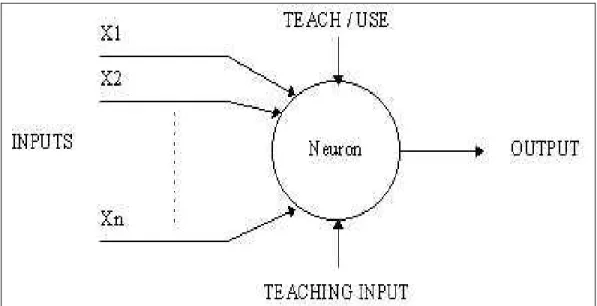
2.3 A Simple Neuron
An artificial neuron is a device with many inputs and one output. The neuron has two modes of operation; the training mode and the using mode. In the training mode, the neuron can be trained to fire (or not), for particular input patterns. In the using mode, when a taught input pattern is detected at the input, its associated output becomes the current output. If the input pattern does not belong in the taught list of input patterns, the firing rule is used to determine whether to fire or not.
6
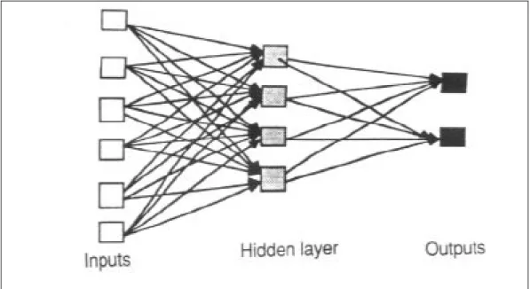
3. ARCHITECTURE OF NEURAL NETWORKS 3.1 Feed-forward networks
In feed forward ANNs as shown in figure 3.1, the information flow is one directional from the input layer to the hidden layer then to the output layer. There is no feedback from the output layer.
These networks are extensively used in pattern recognition.
• Inputs (x): Independent or predictor variables
The input neurons or variables are very important in ANN modeling as the success of an ANN depends to a large extent on the patterns represented by the input variables. What and how many variables to use should be determined carefully. For a forecasting problem, we need to specify a set of appropriate predictor variables and use them as the input variables. On the other hand, for a time series forecasting problem, we need to identify a number of past lagged observations as the inputs. In either situation, it is very critical to determine the best number of input neurons. (Zhang, G. Peter, 2003)
• Hidden layer:
Neurons in the hidden layer are connected to both input and output neurons and are key to learning the pattern in the data and mapping the relationship from input variables to the output variable. With nonlinear transfer functions, hidden neurons can process complex information received from input neurons and then send processed information to the output layer for further processing to generate forecasts. (Zhang, G. Peter, 2003)
7
Figure 3.1 An example of a simple feed forward network
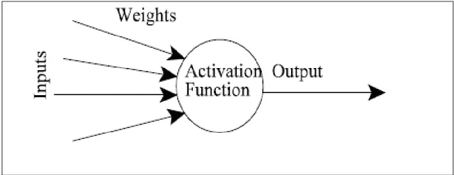
The inputs are multiplied by weights (strength of the respective inputs), and then computed by a mathematical function that determines the activation of the neuron. Another function (which can be the identity=1) computes the output of the neuron. ANNs combine these artificial neurons to process information.
The higher the weight of the neuron is, the stronger the relative input. If the weight is negative, we can say the signal is inhibited by the negative weight. By adjusting these weights, the required output can be obtained. In order to adjust the weights of the ANN of hundreds or thousands of neurons, an algorithm should be set up, which is called “learning” or “training” algorithm.
Although the estimation process of the weights is similar o the one in linear regression where the sum of squared errors is minimized, the ANN training process is more complicated due to the non-linear optimization involved.
8 There are many different training algorithms, but “back propagation algorithm” is the most common one. (Gershenson, 2003)
Figure 3.2 An artificial neuron
3.1.1 The Back propagation Algorithm
The back propagation algorithm (Rumelhart and McClelland, 1986) is used in layered feed-forward ANNs. The neurons are organized in layers which send their signals forward; and the errors are propagated backwards.
The network is fed with the inputs and the desired outputs. Then, the error between actual and desired outputs is calculated. The aim of the algorithm is to reduce this error by adjusting the weights, until ANN learns the training data.
The training process starts with random weights and ends when the weights are adjusted so that the error (actual output minus desired output) is at minimum.
9
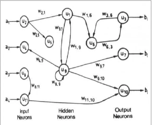
3.2 Feedback Networks
Feedback networks (figure 3.2) can have signals travelling in both directions by introducing loops in the network. Feedback networks are very powerful and can get extremely complicated. Feedback networks are dynamic; their 'state' is changing continuously until they reach an equilibrium point. They remain at the equilibrium point until the input changes and a new equilibrium needs to be found. Feedback architectures are also referred to as interactive or recurrent, although the latter term is often used to denote feedback connections in single-layer organizations. (Stergiou,Siganos,1996).
10
3.3 Perceptrons
The perceptron is a type of artificial neural network invented in 1957 at the Cornell
Aeronautical Laboratory by Frank Rosenblatt. It can be seen as the simplest kind of feedforward neural network: a linear classifier. There is no hidden layer.
Using the simple two-layer perceptron as an example, there is one layer of input nodes (layer 1) and one layer of output nodes (layer 2). Each layer is fully connected between the other, but no connections exist between nodes in the same layer. When layer 1 sends a signal to layer 2, the associated weights on the connections are applied and each receiving node on layer 2 sums up the incoming values. If the sum exceeds a given threshold, that node in turn fires an output signal. (Estebon, 1997)
11
4. FORECASTING APPLICATIONS OF NEURAL NETWORKS
Prediction is a special type of dynamic filtering where past values are used to predict future ones. It is commonly used in forecasting where one has a time series that extends to the present and one wants to predict the time series for future samples.
One typical example of forecasting is for instance predicting the behavior of the stock market or forex market.
Predicting the future output of very complex systems is a difficult task. Adaptive systems however have shown themselves, trained on the right data, quite capable of producing good predictions. They are consistently better than more traditional methods. (peltarion.com, applications of adaptive systems)
A wide range of business forecasting problems have been solved by neural networks. Some of these application areas include:
• Accounting (forecasting accounting earnings, earnings surprises; predicting bankruptcy and business failure),
• Finance (forecasting stock market movement, indices, return, and risk; exchange rate; futures trading; commodity and option price; mutual fund assets and performance),
• Marketing (forecasting consumer choice, market share, marketing category, and marketing trends),
• Economics (forecasting business cycles, recessions, consumer expenditures, GDP growth, inflation, total industrial production, and US Treasury bond),
• Production and operations (forecasting electricity demand, motorway traffic, inventory, new product development project success, IT project escalation, product demand or sales, and retail sales),
• International business (predicting joint venture performance, foreign exchange rate), real estate (forecasting residential construction demand, housing value),
12
• Tourism and transportation (forecasting tourist, motorway traffic, and international airline passenger volume),
• Environmental related business (forecasting ozone level and concentration, air quality).
(Zhang, G. Peter, 2003)
4.1 Literature Review
The exchange rate market, together with the stock market, have been widely used as the forecasting object in a various forecasting studies. This is driven by their nonlinear structures, which make them difficult to predict, and also the profit opportunities that arise from the successful prediction of the markets’ future movement.
There are three main ideas in terms of the predictability of the exchange rate market and financial markets in general. First one is efficient-market hypothesis (EMH) (Fama, 1970, 1991), which asserts that financial markets are "informationally efficient". There are no profit opportunities that could arise from forecasting the exchange rate market and no models could outperform random walk (RW) model.
The other two schools of thought attempt to contradict the above argument, claiming that the market is not always efficient and that by using relevant fundamental variables (fundamental analysis) or chartist approaches (technical analysis) researchers can outperform the RW model.
In Fundamental analysis, which focuses on the economic forces of supply and demand that causes price movement, there are two main shortcomings. First, as most fundamental variables are available in a monthly or annual basis, they are mainly applicable to long-term forecasting rather than short-term forecasting. And secondly research evidence suggest that they are inadequate to beat the RW model in out of sample data sets (Meese and Rogoff, 1983).
13 Technical analysis, which is the analysis of a financial market by charting its performance using historical patterns and focusing on trends, have shown that issuing buy and sell signals which are generated by technical indicators can outperform the out of sample performance of the RW model as well as that of other popular econometric approaches (i.e. GARCH model) (Brock et al.,1992; Gencay, 1996).
Despite their success, the above models do not possess a solid statistical background. This inefficiency led the researchers to apply statistical models with the Box and Jenkins modelling approach (i.e. ARIMA model) (Box et al., 1994),
Due to the high volatility of the market, researchers developed more advanced statistical tools in order to capture the market’s volatility by designing models that can forecast the conditional variance of the series (i.e. GARCH model) rather than the conditional mean (ARMA models) (Bollerslev, 1986; Engle, 1982). Hsieh (1989) combined both AR and GARCH models by firstly estimating an AR model and then applying a GARCH model on the residuals. The GARCH model was able to outperform the RW model in three out of the five exchange rates under investigation. However, diagnostics tests revealed that there was still some form of nonlinear information in the residuals. Statistical models still have their limitations like any other forecasting methods. Hu, Zhang, Jiang, and Patuwo (1999) suggest that the failure of these models is not only due to their linear structure, as nonlinear statistical approaches such as GARCH models also failed to outperform the RW model; but their a priori assumption of the model’s structure. Yao and Tan (2000) have also argued that the nature of financial data which have high volatility, complexity, noisy environments, etc. cannot be described by simple linear structural models, autoregressive and moving average processes, or even simple white noise processes. Based on that Neural Networks, as data driven nonparametric modelling approaches that require no a priori assumption about the system’s structure, have been considered as a more appropriate approach for the approximation of the nonlinear and complex functions including the financial systems (Zhang et al., 1998). (Anastasakis, Mort, 2009)
Gunter (1989) suggested that it may be more beneficial to combine different sets of combined forecasts rather than picking one of them. He used N-step combinations of
14 forecasts which involves recombinations of the different combinations of the original forecasts of a time series and concluded that two-step combinations improve upon one-step combinations and original forecasts of GNP (gross national product).
Bellgard and Goldschmidt (1999) also examined the forecasting accuracy and trading performance of several forecasting techniques including exponential smoothing, random walk, ARMA models and Neural Networks. Their study was based on Australian Dollar/ US Dollar exchange rate and they concluded that foreign exchange time series show non-linear patterns that are better exploited by neural network models.
Also, Dunis and Williams (2002) showed that Neural Network models can add value to the forecasting process, and that for the EUR/USD exchange rate prediction; Neural Network models outperform the more traditional modeling techniques.
Gradojevic and Yang (2000) combined artificial neural networks and market microstructure to exchange rate determination to explain short-run exchange rate movements. They included a variable from the field of microstructure, order flow in a set of macroeconomic variables such as interest rate and crude oil price to explain Canada/U.S.Dollar exchange rate movements. Their results showed that ANN models never performed worse than linear models, and always better than random walk model. There are many other researches on various different cases that show the success of Neural Networks in different application areas from business to tourism and marketing.
15
5. COMPLEXITY, CHAOS AND NON LINEARITY
5.1. Complexity
A complex system is a system composed of interconnected parts that as a whole exhibit
one or more properties (behavior among the possible properties) not obvious from the properties of the individual parts.(http://www.wikipedia.org)
A complex system is fundamentally non-deterministic. It is impossible to anticipate precisely the behavior of such systems even if we completely know the function of its constituents. It has a dynamic structure. It is therefore difficult to study its properties by decomposing it into functionally stable parts. The relationships that exist within the elements of a complex system are short-range, non linear and contain feedback loops. (http://www.irit.fr)
5.2. Chaos Theory
The Greek word of chaos, that can be translated as disorder and lawlessness shows ancient Greek understanding of the universe. According to this point of view, although world’s entities seem to be chaotic, random and as a result unpredictable, they are at the same time in order and deterministic. (Torkamani et al., 2007)
Chaos theory attempts to explain the fact that complex and unpredictable results can and will occur in systems that are sensitive to their initial conditions. A small change in the initial conditions can drastically change the long-term behavior of a system.
Unstable aperiodic behavior is highly complex as it never repeats in time. A chaotic system is very sensitive to initial conditions.
This sensitivity to initial conditions is popularly known as the "butterfly effect", so called because of the title of a paper given by Edward Lorenz in 1972 entitled
16 Predictability: Does the Flap of a Butterfly’s Wings in Brazil set off a Tornado in Texas?
In his study on climate, he showed that atmospheric events are highly unpredictable; all forecasts are valid only for a few days and very sensitive to initial conditions. Tiny changes that would even not be noticed might lead to extensively different states of behaviors. However, this unpredictability is limited within specific boundaries. (in February, a temperature in Siberia can be anything but not as high as 400C). This phenomena, in fact, is described as “instability within stability” or a “mixture of order and disorder” and represents the main characteristic of chaos.
The flapping wing represents a small change in the initial condition of the system, which causes a chain of events leading to large-scale phenomena. Had the butterfly not flapped its wings, the trajectory of the system might have been vastly different. (http://www.wikipedia.org)
The same principles characterizing chaotic behavior and instability are applicable to the model of the economy. Healthy capital markets and money markets are characterized by turbulence and volatility, rather than by efficiency and fair price. Like any dynamic system, a healthy economy does not tend to equilibrium but is, instead, in steady change. That is why economists who are currently using equilibrium theories to model market systems are likely to produce dubious results. (Dimitris, 1994)
5.3. Linearity and Non-linearity
Linear system: Linear system is a system in which the variables plot a straight line.
Predictable changes occur and a small change has a small effect. E.g thermostat
Non-linear system: In non-linear systems, variables are represented by curvilinear
patterns, and feedback loops have unpredictable effects, yet can be replicable. E.g. Starling’s curve for the heart, weather systems, presidential elections, financial systems.
17 Historically, economists have always tried to use linear equations to model economic phenomena; whenever possible. Because linear models are easy to manipulate and they give unique solutions. However, it is not possible to ignore the fact that the economic world; such as many other systems show nonlinear patterns.
There is a strong belief in economics for both the significance of linear models, and the advantages of nonlinear models. But nonlinear models clearly outperform linear models. As the economic world is nonlinear, it would appear that focusing on linear dynamics is of limited interest. However economists have typically found nonlinear models to be so difficult and intractable that they have adopted the technique of linearization to deal with them.
Important phenomena for which linear models are not appropriate include depressions and recessionary periods, stock market price bubbles and corresponding crashes, persistent exchange rate movements and the occurrence of regular and irregular business cycles. Therefore, economic theorists are turning to the study of non-linear dynamics and chaos theory as possible tools to model these and other phenomena. The most exciting feature of nonlinear systems is their ability to display chaotic dynamics. Much economic data has this random-like behavior, but it comes from agents and markets that are presumably rational and deterministic. (Torkamani et al., 2007)
As Neural Networks can be used to model non-linear relationships in data, it will be a perfect tool to use to forecast the exchange rates.
18
6.CURRENCY MARKETS
6.1 Money Market
An individual who has a checking account can be defined as a participant in the money market. The instrument which is bought and sold in this market is called “money” or “near money”.
‘Money is anything that is generally accepted as payment for goods and services and repayment of debts. The main uses of money are as a medium of exchange, a unit of account, and a store of value.’(http://www.en.wikipedia.org)
Near money is a term used to describe highly liquid assets that can easily be converted into cash. (http://www.en.wikipedia.org)
The main actors in the money market are:
• Commercial Banks
• Large Corporations
• Other Financial Instutions
19
6.2 Foreign Money Market
In foreign money market, market instruments are bought and sold outside the country where their currency of denomination is legal tender.
The actors in foreign money market are mainly commercial banks and corporations.
• Commercial Banks
The objectives of commercial banks in foreign money market, as described by Heinz Riehl and Rita M.Rodriguez (1977) are:
-To maintain the liquidity, and therefore the solvency of the bank -To use excess funds so that they produce the highest possible return -To borrow required funds at the lowest possible cost
• Large Corporations
The objectives of large corporations are similar to commercial banks. They have liquidity positions to maintain, but they also have to make sure that their money is invested at the highest possible return.
• Central Banks
Central banks also play an important role in the foreign money markets when they decide to invest their foreign exchange reserves. But this should be noted that no central bank exercises a supervisory or controlling function in foreign money markets. Individuals generally do not participate in foreign money markets as the markets generally show a wholesale nature, that is too large for an average individual and small transactions are too costly.
20
6.3 Foreign Exchange Market
Heinz Riehl and Rita M.Rodriguez (1977) describe foreign exchange market as a market where financial paper denominated in a given currency with a relatively short maturity is traded against paper denominated in another currency.
It can easily be told that if all countries used the same currency, foreign exchange market would not exist.
Exchange rates (or foreign exchange rates) between two currencies can be defined as the value of a foreign nation’s currency in terms of the home nation’s currency
In money market, currency provides immediate purchasing power while a treasury bond for example provides this power at a specified date in future. This “time” elements shows itself in foreign exchange market by dividing the market into spot and forward markets.
In spot market, foreign exchange is delivered within two business days.
In forward market, foreign Exchange is delivered at some specified date in future.
This date in future is called the “value date.” (Riehl and Rodriguez ,1977)
If we consider Turkey exporting goods to United States; Turkey should pay to his employees TL. On the other hand; USA people have USD . Turkey bills the American either in USD or in TL. In either cases; foreign exchange market is necessary to sell USD and purchase TL.
It does sometimes happen that transactions between two countries are settled in a third currency; which is neither the exporter’s nor the importer’s currency. In this case also; where a populer currency is used; exchange market is needed.
21 The actors in foreign exchange (Forex) market are:
• Commercial banks:
The aims of the commercial banks are:
-to give best possible service to customers such as importers or exporters,
-to manage to keep the bank’s inventory of each currency at the desired level; -to make profit while accomplishing the first two objectives.
• Non-financial businesses:
Nonfinancial businesses exist in foreign exchange market through two primary sources: international trade and direct investment.
International trade involves either the payment or the receipt of a foreign currency. And the businesses desire to make the transactions at the most advantageous price of foreign exchange possible.
Foreign direct investment involves the acquisition of an asset or generation of a liability in a foreign currency. In either situation, fluctiations in the value of the foreign currency will affect the value of the company’s foreign operations. To avoid these risks; businesses will keep dealing in the foreign exchange market.
• Central banks
Central Banks are responsible for maintaining the value of the domestic currency against the foreign currencies. This is certainly true under the system of fixed exchange rates. Even within the system of floating exchange rates, the central banks have usually felt compelled to intervene in the foreign exchange market at least to maintain orderly markets.
22 Under a system of floating exchange rates, the external value of a currency is determined, like the price of any other good in a free market: by the forces of supply and demand. If more domestic currency is offered than demanded; that is if more foreign currency is demanded than offered (for example if imports were to exceed exports), then the value of the domestic currency in terms of foreign currency will tend to decrease. This means, it will take fewer units of foreign currency to acquire one unit of domestic currency. The role of the central bank should be minimum unless it has certain preferences for what the foreign exchange rate should be. For example, if the central bank desires to protect the local export industry, it will try to make the domestic currency cheaper relative to foreign currencies by selling its local currency on exchange markets.
Under a system of fixed exchange rates, the central bank is obliged to maintain the value of the domestic currency within a narrow band of fluctiations. Whenever the transactions of financial and nonfinancial institutions do not produce a balance between supply and demand for exchange rate, the central bank should absorb the difference.
If there’s excessive supply of local currency in the market, central bank has to absorb the surplus by selling out its stock of foreign exhange, probably at rising prices. It will purchase local currency and sell foreign currencies. This results in an outflow of foreign currency, decrease in foreign exchange reserves, and the need to devaluate the local currency or deflate the domestic economy.
If there’s excessive demand for local currency, the central bank has to provide the shortfall by accumulating foreign Exchange and providing local currency at rising prices. It will sell local curreny and buy foreign currencies. This results in an inflow of foreign currency, increase in country’s foreign exchange reserves, and pressure to upvalue the local currencynor increase domestic prices. Domestic Money supply will
23 thus increase, economy will be fuelled and inflation will be stimulated. (Riehl and Rodriguez , 1977)
6.4. A Brief History of Exchange Rates
6.4.1 The Gold Standard, 1876-1913
The gold standard is a system in which international currencies are fixed to a specific amount of gold. In this system, all participating currencies were convertible to each other based on their gold values.
In theory, all nations should have an optimal balance of payments of zero; they should not have either a trade deficit or trade surplus. For example, if a Brazil had a trade deficit with Australia, Brazil should pay Australia gold. When Australia had more gold, it could issue more paper money since it now had a greater supply of gold. With an increase of money supply in the Australian economy, inflation would occur. This rise in prices would subsequently lead to a drop in exports, because Brazil would not want to buy the more expensive Australian goods. As a result, Australia would then return to a zero balance of payments as its trade surplus would disappear. Likewise, when gold leaves Brazil, the price of goods should decline, making them more attractive for Australia. Consequently, Brazil would experience an increase in exports until its balance of payments reached zero. Therefore, the gold standard would ideally create a natural balancing effect to stabilize the money supply of participating nations.
But in reality, the gold standard had many problems. When gold left a nation, the ideal balancing effect would not occur immediately. Instead, recessions and unemployment were often seen. Instead of changing tax rates or increasing expenditures to stimulate growth - governments chose to not interfere with their nations' economies. Thus, trade deficits would persist, resulting in chronic recessions and unemployment. (Monem, 2007)
24 The gold standard worked until the outbreak of WWI, which interrupted trade flows and free movement of gold thus forcing major nations to suspend operation of the gold standard.
6.4.2 Inter-War Years and World War II, 1914-1944
During WWI, governments took their currencies off the gold standard and simply dictated the value of their money.
In 1934, the US devalued its currency to $35/oz from $20.67/oz prior to WWI.
From 1924 to the end of WWII, exchange rates were theoretically determined by each currency's value in terms of gold.
During WWII and aftermath, many main currencies lost their convertibility. The US dollar remained the only major trading currency that was convertible
6.4.3 Bretton Woods System, 1944-1971
Cooperation and reconstruction (1944–71)
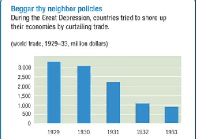
During the Great Depression of the 1930s, countries attempted to support their weakening economies by raising barriers to foreign trade, devaluing their currencies to compete against each other for export markets, and restricting their citizens' freedom to hold foreign exchange. But all these attempts proved to be unsuccessful. World trade declined (figure 6.1), and employment and living standards dropped sharply in many countries.
25
Figure 6.1 The world in depression
This collapse in international monetary cooperation led the IMF's founders to build an institution to manage the international monetary system—the system of exchange rates and international payments that enables countries and their citizens to buy goods and services from each other. The new global entity would ensure exchange rate stability and encourage its member countries to eliminate exchange restrictions that obstructed trade. (www.imf.org)
The Bretton Woods agreement:
In July 1944, representatives of 45 countries met in the town of Bretton Woods, New Hampshire, in the United States, and agreed on a framework for international economic cooperation, to be established after the Second World War. They believed that such a framework was necessary to avoid the repetition of the disastrous economic policies that had contributed to the Great Depression. (http://www.imf.org)
Par value system (Bretton Woods System)
The international monetary system known as the Bretton Woods system was based on stable and adjustable exchange rates. Exchange rates were not permanently fixed, but
26 occasional devaluations of individual currencies were allowed to correct fundamental disequilibrium in the balance of payments. (http://www.econ.iastate.edu)
Under the Bretton Woods system, the world currencies were tied to the dollar, and dollar was convertible into gold at $35 per ounce.
The central banks of countries other than the United States were given the task of maintaining fixed exchange rates between their currencies and the dollar. They did this by intervening in foreign exchange markets. If a country's currency was too high relative to the dollar, its central bank would sell its currency in exchange for dollars, driving down the value of its currency. Conversely, if the value of a country's money was too low, the country would buy its own currency, thereby driving up the price. (http://www.economics.about.com)
6.4.4 The end of the Bretton Woods System (1972–81)
By the early 1960s, the U.S. dollar's fixed value against gold, under the Bretton Woods system of fixed exchange rates, was seen as overvalued. A sizable increase in domestic spending on President Lyndon Johnson's Great Society programs and a rise in military spending caused by the Vietnam War gradually worsened the overvaluation of the dollar. (http://www.imf.org)
End of Bretton Woods system:
The system dissolved between 1968 and 1973. In August 1971, U.S. President Richard Nixon announced the "temporary" suspension of the dollar's convertibility into gold. While the dollar had struggled throughout most of the 1960s within the parity established at Bretton Woods, this crisis marked the breakdown of the system. An attempt to revive the fixed exchange rates failed, and by March 1973 the major currencies began to float against each other. (http://www.imf.org)
27 The resulting system was called “managed float regime," meaning that even though exchange rates for most currencies float, central banks still intervene to prevent sharp changes. As in 1971, countries with large trade surpluses often sell their own currencies in an effort to prevent them from appreciating (and thereby hurting exports). Countries with large deficits often buy their own currencies in order to prevent depreciation, which raises domestic prices (http://www.economics.about.com)
After the collapse of the Bretton Woods system, IMF members have been free to choose any form of exchange arrangement they wish (except pegging their currency to gold): allowing the currency to float freely, pegging it to another currency or a basket of currencies, adopting the currency of another country, participating in a currency bloc, or forming part of a monetary union. (http://www.imf.org)
6.4.5 Floating Exchange Rate Regime, 1973-Present
The dollar was devalued a first time in 1971, a second time in 1973 to eventually started floating. Since 1973, the world has experienced more volatile exchange rates.
A floating exchange rate is determined by the private market through supply and demand. A floating rate is often termed "self-correcting", as any differences in supply and demand will automatically be corrected in the market. If demand for a currency is low, its value will decrease, thus making imported goods more expensive and thus stimulating demand for local goods and services. This in turn will generate more jobs, and hence an auto-correction would occur in the market. A floating exchange rate is constantly changing.
28 In reality, no currency is wholly fixed or floating. In a fixed regime, market pressures can also influence changes in the exchange rate. Sometimes, when a local currency does reflect its true value against its pegged currency, a "black market" which is more reflective of actual supply and demand may develop. A central bank will often then be forced to revalue or devalue the official rate so that the rate is in line with the unofficial one, thereby halting the activity of the black market.
In a floating regime, the central bank may also intervene when it is necessary to ensure stability and to avoid inflation; however, it is less often that the central bank of a floating regime will interfere. (Reem Heakal, 2003)
6.5. The Chaotic Behaviour of Foreign Exchange Rates
The foreign exchange market is the largest and most liquid of the financial markets. Foreign exchange rates are amongst the most important economic indices in the international monetary markets. The forecasting of them poses many theoretical and experimental challenges. Foreign exchange rates are affected by many highly correlated economic, political and even psychological factors. The interaction of these factors is in a very complex fashion. Therefore, to forecast the changes of foreign exchange rates is generally very difficult. Researchers and practitioners have been striving for an explanation of the movement of exchange rates. Thus, various kinds of forecasting methods have been developed by many researchers and experts. Like many other economic time series, forex has its own trend, cycle, season, and irregularity. Thus to identify, model, extrapolate and recombine these patterns and to give forex forecasting is the major challenge. (Torkamani et al.,2007)
As discussed in chapter 5, in many problems, the behaviour of systems are accepted as linear although their true characteristics are non-linear, because of the difficulty in modelling non-linear behaviours. But this trend is changing since powerful computers and new modelling tools such as neural networks are available and usable for tackling
29 complex calculations. Unlike a linear relationship in which a given cause has only one effect, in a non-linear relationship, a cause may have more than one outcomes. Thus non-linear equations can have more than one solution. (Karaguler, 2000)
In the early 1970s, many economists believed that the floating currency exchange rates that were to characterize the post-Bretton Woods period could be well explained by the purchasing power parity theory [see Bilson and Marston, 1984]. As empirical data soon demonstrated, however, the theory was not sufficient to explain the large fluctuations in exchange rates, new theories suggested that a country's exchange rate was the market price of local money in the world market. Among the determinants of this price a key element was seemed to be the supply of and the demand for the local currency. The theories also accounted for the effects of other economic variables, and rational expectations. ( Aczel and Josephy, 1991 )
Foreign exchange rates were only determined by the balance of payments at the very beginning. The balance of payments was merely a way of listing receipts and payments in international transactions for a country. Payments involve a supply of the domestic currency and a demand for foreign currencies. Receipts involve a demand for the domestic currency and a supply of foreign currencies. The balance was determined mainly by the import and export of goods. Thus, the prediction of the exchange rates was not very difficult at that time. Unfortunately, interest rates and other demand} supply factors had become more relevant to each currency later on. On top of this the fixed foreign exchange rates was abandoned and a floating exchange rate system was implemented by industrialized countries in 1973. Recently, proposals towards further liberalization of trades are discussed in General Agreement on Trade and Tariffs. Increased Forex trading, and hence speculation due to liquidity and bonds, had also contributed to the difficulty of forecasting Forex . (Torkamani et al., 2007)
30
7. APPLICATION OF ARTIFICIAL NEURAL NETWORKS TO EXCHANGE RATE FORECASTING
Understanding exchange rate movements has always been an extremely challenging and important task .Many forecasting models have been built to understand the inner mechanism of exchange rate movements.
Artificial neural networks is an optimal tool for modelling the complex and non-linear relationships in exchange rates as also discussed in previous chapters . The “learning from data or experience” feature of ANNs is highly desirable in our case, where past data is easy to collect, but the underlying data-generating mechanism is not known or pre-specifiable. Also, neural networks have been mathematically shown to have the universal functional approximating capability in that they can accurately approximate many types of complex functional relationships. This is an important and powerful characteristic, as any forecasting model aims to accurately capture the functional relationship between the variable to be predicted and other relevant factors or variables.
In this thesis, I will use EUR/USD parity, the interest rate in Turkey, the interest rate in USA, increase in inflation rates in Turkey, GDP changes in Turkey and USA and the current USD/TRY parity as my input variables to forecast the USD/TRY parity in future using the Neuro Solutions program.
31
7.1. Building a Neural Network
To build a neural network, we should first identify the type of problem.
In prediction problems, the goal is to determine an output given a set of inputs and the past history of the inputs. The prediction problems use the current input and previous inputs (the temporal history of the input) to determine either the current value of the output or a future value of a signal.
In our case, the current values of the USD/TRY exchange rate, together with other economical indicators will be used to forecast the USD/TRY exchange rate one week from now.
Our inputs for the model are EUR/USD parity, the interest rate in Turkey, the interest rate in USA, increase in inflation rates in Turkey, GDP changes in Turkey and USA and the current USD/TRY and our desired output is the USD/TRY parity one week from now.
After selecting our input and output variables, we should set aside some percentage of our data for cross-validation and testing.
One of the primary goals in training neural networks is to make sure that the network performs well on data that it has not been trained on; which is called generalization. The standard method of ensuring good generalization is to divide the training data into multiple data sets. The most common data sets are the training, cross validation, and testing data sets.
“Cross-validation is a test of validity for a regression model that involves using comparable data to check the validity of an original estimation.“
32 The cross validation data set is used by the network during training. Periodically, while training on the training data set, the network is tested for performance on the cross validation set. During this testing, the weights are not trained, but the performance of the network on the cross validation set is saved and compared to past values. If the network is starting to overtrain on the training data, the cross validation performance will begin to degrade. Thus, the cross validation data set is used to determine when the network has been trained as well as possible without overtraining (i.e., maximum generalization).
Every 5 epochs, the learning will be turned off and the network will be tested on the cross validation data set. The network is "optimal" when the error in the cross validation set is at its minimum position.
The Generalization Protection panel is used to specify the amount of data to set aside for cross validation. "None" indicates that all of the data in the input and desired files will be used for training. This option is generally only used when you have very little data to work with (e.g., less than 100 rows). "Normal" generalization protection specifies that 20% of your data will be set aside for cross validation. "High" generalization protection will set aside 40% of your data for cross validation. This option should only be used when you have a great deal of data (e.g. 10,000 rows or more).
In our case, normal generalization (20% of the data) will be used for cross validation. And the remaining data will be used for training and testing.
Although the network is not trained with the cross validation set, it uses the cross validation set to choose a "best" set of weights. Therefore, it is not truly an
out-of-33 sample test of the network. For a true test of the performance of the network the testing set is used.
Testing data will not be used during training; so this provides a true indication of how the network will perform on new data.
The Network Complexity panel is used to specify the size of the neural network in
terms of hidden layers and processing elements (neurons). In general, smaller neural networks are preferable over large ones. If a small one can solve the problem sufficiently, then a large one will not only require more training and testing time but also may perform worse on new data. This is the generalization problem -- the larger the neural network, the more free parameters it has to solve the problem. Excessive free parameters may over fit the data, causing the network to overspecialize or memorize the training data. When this happens, the performance of the training data will be much better than the performance of the cross validation or testing data sets.
34
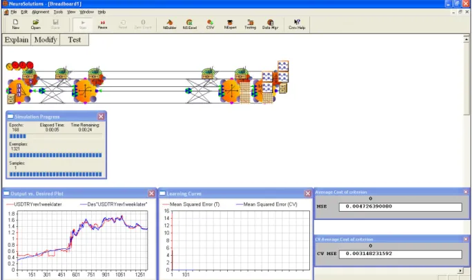
Figure 7.1 The breadboard at the beginning of the simulation
35
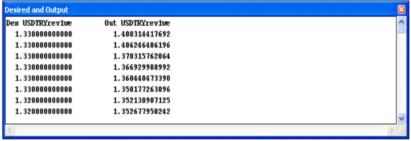
Figure 7.3 Desired vs actual output of the program
7.2. Explanations of the Breadboard 7.2.1. Input Axon (Prediction)
Figure 7.4 Input axon
This component is a Lagurre axon that accepts the inputs to the network, delays and processes them, and passes them on to the network. This element gives the network memory into the past history of the data, allowing the network to extract relationships in time.
7.2.2. First Hidden Layer (Prediction)
36 The synapse makes the connection between each input and each processing element (PE) in the hidden layer. The synapse contains the connections and the trainable weights for each connection.
Figure 7.6 The tanh axon
The second component is the tanh axon. This component has the processing elements for the hidden layer, each of which sums the weighted connections from the inputs.
7.2.3. Output Layer (Prediction)
Figure 7.7 The synapse
The synapse is the first component and provides the connection. The synapse contains the connections and the trainable weights for each connection.
Figure 7.8 The bias axon
The second component is the bias axon. This component has the processing elements for the output layer.
37
7.2.4.Criterion
Figure 7.9 The criterion
This component is the criterion. It accepts the output(s) of the network and the desired output(s) and compares them. It computes the error and passes this error to the backpropagation components which adjust the weights of the network for training.
7.3. Training Report
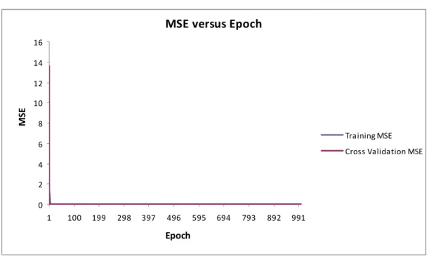
38 This plot shows the mean squared error (MSE) of the network after each epoch of data. The epoch number is shown on the X-axis and the MSE is shown on the Y-axis. The MSE of the training set is shown in red and the MSE of the cross-validation set is shown in blue. A network that is training well should have a constantly decreasing slope of the training MSE (typically an exponential decay); which is the case in our model.
! " "
# " "
Table 7.2 Mean squared error of training and cross validation sets
The epoch when the training error was at its minimum was at 985 during training and 987 during cross validation.
The minimum training error is 0.00085624 and minimum cross validation error is 0.000831683.
The final value of the mean squared error (MSE) of the network using the training set is 0.000856644 and using the cross validation set is 0.000917823.
39 7.4. Testing Report " " " " " " " " $ % &' () * ((+ ( $ % &' () * ((+ (
Table 7.3 Output vs desired plot
This probe plots the output of the network and the desired output of the network on the same plot. When the network is performing well, these two curves should be very similar – implying that the output of your network is very close to the desired output of your network.
40
" mean squarred error
, "
Normalized Mean squared error (MSE/variance of desired output)
- " Mean absolute error
-. " / Minimum absolute error
0 -.
" Maximum absolute error
" Linear correlation coefficient
Table 7.4 Test report
7.5. Putting the Network Model for Use
After building, training and testing our model, we will be able to forecast the USD/TRY parity one week from now.
! ! 1 ( (
2 ! ! ! 3
( ! ! ( * ((+ (
2 ( ( ! ! 3
! "# ! $ "
Table 7.5 Output of the model
41
8. CONCLUSION
Artificial Neural Networks are modeling tools inspired from the human brain. They are capable of handling complex problems and they can process several inputs at the same time to generate an appropriate output. They can learn by example using past data and can be used to model non-linear, complex systems.
Forecasting of exchange rates was a challenging study with many complications because of their chaotic, non-linear behaviors. This is where the idea of using artificial neural networks came to the forefront.
In this thesis, I used artificial neural networks to model and forecast the USD/TRY exchange rate one week from now. The inputs EUR/USD parity, the interest rate in Turkey, the interest rate in USA, increase in inflation rates in Turkey, GDP changes in Turkey and USA and the current USD/TRY parity have been used to forecast the USD/TRY parity in future using the Neuro Solutions program.
When the outputs of the model were compared with the actual outputs after the training phase was completed, the curves showing the desired out put and the actual output looked identical; which proved the success of the model. The final value of the mean squared error (MSE) of the network using the training set was 0.000856644 and using the cross validation set it was 0.000917823. The MSE of the testing set was 0.002068077. The model was able to forecast the USD/TRY with 98% accuracy.
Further studies may be applicable to this thesis using the same data with other modeling and forecasting methods. The results can be compared then, to see which method was superior in our case study.
42
REFERENCES
Amir D. Aczel and Norman H. Josephy. 1991, ‘The Chaotic Behavior of Foreign Exchange Rates’ , American Economist, Vol. 35.
Applications of adaptive systems. 2008. 15 March 2009 http://www.peltarion.com. Artificial Neural Network. 2009. 10 March 2009 http:// www.en.wikipedia.org.
Bellgard, C. and Goldschmidt, P.1999 , Forecasting Across Frequencies: Linearity and Non-Linearity.
Bilson and Marston. 1984, Exchange Rate Theory and Practice.
Bollerslev, T. 1986. ‘Generalised autoregressive conditional heteroskedasticity’ , Journal of Econometrics, 31(3), 307–327.
Box, G. E. P., Jenkins, G. M., and Reinsel, G. C. 1994, Time series analysis: Forecasting and Control, Englewood Cliffs, NJ: Prentice Hall.
Brock, W., Lakonishok, J., LeBaron, B.1992, ‘Simple technical trading rules and the stochastic properties of stock returns’ , Journal of Finance, 47(5), 1731–1764.
Chorafas, Dimitris N. 1994, Chaos Theory in the Financial Markets, Irwin Professional Publishing, United States of America
Christian L. Dunis and Mark Willaims .2002, ‘Modelling and Trading the EUR/USD Exchange Rate: Do Neural Network Models Perform Better?’ , Liverpool Business School and CIBEF.
Cooperation and reconstruction of IMF. 2010. 16 March 2009 http://www.imf.org/external/about/histcoop.htm
43 Engle, R. F. 1982, ‘Autoregressive conditional heteroskedasticity with estimates of the variance of United Kingdom inflation’ , Economertrica, 50(4), 987–1008.
Estebon, Michele D. 1997, ‘Perceptrons: An Associative Learning Network’ , Virginia Tech, CS 3604
Fama, E. F. 1970, ‘Efficient capital markets: A review of theory and empirical work’ , Journal of Finance, 25(2), 383–417.
Gershenson, Carlos. Artificial Neural Networks for Beginners. 2003 10 April 2009 http://arxiv.org/ftp/cs/papers.
Gradojevic, Nikola and Yang, Jing. 2000, ‘The Application of Artificial Neural
Networks to Exchange Rate Forecasting: The Role of Market Microstructure Variables’ , Bank of Canada Working Papers, 00-23.
Gunter, Sevket I. and Aksu, Celal. 1989, ‘N-Step Combinations of Forecasts’ , Journal of Forecasting, Vol. 8, 253-267.
Heinz Riehl and Rita M. Rodriguez. 1977, Foreign Exchange Markets, A Guide to Foreign Currency Operations.
Hu, M. Y., Zhang, G. P., Jiang, C. X., and Patuwo, B.E.1999, ‘A cross-validation analysis of neural network out-of-sample performance in exchange rate forecasting’ , Decision Sciences, 30(1), 197–216.
Karaguler, Turhan. 2000, ‘Chaos Theory and Exchange Rate Problem’ , International Joint Symposium on Bus. Admin. , Haziran 2000, Gökçeada.
Leonidas Anastasakis ,Neil Mort .2009, ‘Exchange rate forecasting using a combined parametric and nonparametric self-organising modelling approach’ , Expert Systems with Applications, 36, 12001–12011.
44 Lorenz, E. N. 1972, ‘Deterministic Non-period Flows’ , Journal of Atmospheric
Sciences, 20.
Makridakis, S., A. Andersen, R. Carbone, R. Fildes, M. Hibon, R. Lewandowski, J. Newton, E. Parzen, and R. Winkler. 1982, ‘The accuracy of extrapolation (time series) methods: results of a forecasting competition’ , Journal of Forecasting, 1, 111–153. Market research glossary.2009. 17 April 2009
http://www.esomar.org/index.php/glossary-c.html.
Meese, R. A., and Rogoff, K. 1983, ‘Empirical exchange rate models of the seventies: Do they fit out of sample?’ , Journal of International Economics, 14(1–2), 3–24.
Meese, R. A., and Rogoff, K. 1988, ‘Was it real? The exchange rate-interest differential relation over the modern floating-rate period.’ , Journal of Finance, 43(4),933–948. Meese, R. A., and Rose, A. K. 1990, ‘Nonlinear, nonparametric, nonessential exchange rate estimation’ , American Economic Review, 80(2), 192–196.
Monem, Tarik Abdel. What is The Gold Standard?. 2009. 2 May 2009 http://www.uiowa.edu/ifdebook.
Neurosolutions 5 Program Tutorial
Nonlinear systems and neural networks, 2010, 15 June 2009, http://www.irit.fr. Reem Heakal, Floating And Fixed Exchange Rates. 2003. 16 May 2009
http://www.investorwords.com/tips/481/floating-and-fixed-exchange-rates.html.
Rumelhart, D. E., and J. L. McClelland. 1986, ‘Parallel Distributed Processing’ , MIT Press, Ch. 8, pp. 318-362.
45 Russell, Ingrid. 1996, ‘Neural Networks Module’ , University of Hartford’s Academic Web Server , http://uhaweb.hartford.edu/compsci/neural-networks-history.
Stergiou , Christos and Siganos, Dimitrios. ‘Neural Networks’ .1996. 15 March 2009 http://www.doc.ic.ac.uk/~nd/surprise_96/journal/vol4/cs11/report.html.
The Bretton Woods System. 2009. 16 May 2009
http://economics.about.com/od/foreigntrade/a/bretton_woods.htm. The Bretton Woods System. 2009. 16 May 2009
http://www.econ.iastate.edu/classes/econ355/choi/bre.htm.
Torkamani, M.A., Mahmoodzadeh, S, Pourroostaei, S. and Lucas, C. 2007, ‘Chaos Theory and Application in Foreign Exchange Rates vs. IRR (Iranian Rial)’ , World Academy of Science, Engineering and Technology, 30 2007.
Yao, J., and Tan, C. L. 2000, ‘A case study on using neural networks to perform technical forecasting of forex.’ , Neurocomputing, Volume 34(1–4), 79–98.
Zhang, G. Peter. 2003, Neural Networks in Business Forecasting, Hershey, PA, USA, Idea Group Inc.
Zhang, G., and Hu, M. Y. 1998, ‘Neural network forecasting of the British Pound/US Dollar exchange rate’ , Omega The International Journal of Management Science, 26(4), 495–506.