EUROPEAN ORGANIZATION FOR NUCLEAR RESEARCH (CERN)
CERN-EP-2018-144 2018/11/01
CMS-TRK-17-001
Precision measurement of the structure of the CMS inner
tracking system using nuclear interactions
The CMS Collaboration
∗Abstract
The structure of the CMS inner tracking system has been studied using nuclear in-teractions of hadrons striking its material. Data from proton-proton collisions at a center-of-mass energy of 13 TeV recorded in 2015 at the LHC are used to reconstruct millions of secondary vertices from these nuclear interactions. Precise positions of the beam pipe and the inner tracking system elements, such as the pixel detector support tube, and barrel pixel detector inner shield and support rails, are determined using these vertices. These measurements are important for detector simulations, detector upgrades, and to identify any changes in the positions of inactive elements.
Published in the Journal of Instrumentation as doi:10.1088/1748-0221/13/10/P10034.
c
2018 CERN for the benefit of the CMS Collaboration. CC-BY-4.0 license ∗See Appendix A for the list of collaboration members
1
1
Introduction
Precision mapping of the material within the tracking volume of the CMS detector [1] is impor-tant for the experiment’s measurement goals. The material affects the reconstruction of events through multiple scattering, energy loss, electron bremsstrahlung, photon conversions, and nuclear interactions (NIs), of the particles produced in proton-proton collisions. The analysis presented here uses reconstructed NIs to precisely measure the positions of inactive elements surrounding the proton-proton collision point, such as the beam pipe and the inner mechanical structures of the pixel detector. This information is needed to validate simulations of the CMS detector and to identify any shifts in the positions of inactive elements. It can also be used in searches for long-lived particles with displaced vertices [2, 3].
An accurate simulation of the effects of inactive material is necessary for a proper reconstruc-tion of all particles produced in a proton-proton collision event. In particular, the material clos-est to the interaction region affects the track position resolution, which, in turn, strongly affects the b tagging performance [4]. Substantial effort has been invested into the implementation of the detailed GEANT4 [5, 6] geometry used to simulate the detector response. Previous studies
have addressed the systematic uncertainties related to the tracker material simulation [7], val-idation of the simulation with early data [8], and more accurate calibrations based on the data to improve the resolution of calorimeter-based observables [9].
Identifying shifts in the positions of inactive elements is important not only for accurate detec-tor response simulation, but also for CMS tracker upgrade designs. Since the pixel detecdetec-tors are installed with the beam pipe already in place, an accurate measurement of the beam pipe position is of paramount importance. As a consequence of the beam pipe mechanical char-acteristics and support structure design, its final position can be different from the nominal one at the millimeter level [10]. For the design of the Phase-1 upgrade of the pixel detector, which was installed in Spring 2017, NI imaging was used to conclude that the sagging of the beam pipe between the supports was small enough to be of no concern. Both the original and new versions of the CMS pixel detector are split into two half-cylinders and inserted by slid-ing these two halves into place by means of appropriate rails. This installation method does not provide accuracy and reproducibility of the pixel detector positioning below the level of a few millimeters. The evaluation and understanding of these position uncertainties, which are comparable with mechanical clearances between the pixel detector and the beam pipe, were important inputs for the design of the new support system and helped to establish reliable installation procedures for the Phase-1 upgrade of the pixel detector. Clearances may change during detector operation because of deformation due to gravity, and variations in vacuum pressure, temperature, and magnetic field [10]. The innermost layer of the Phase-1 upgrade of the pixel detector is even closer to the beam pipe than the previous innermost pixel layer [10], but the clearances were well understood from the NI imaging of the pixel detector support tube.
Nuclear interaction reconstruction has been developed in the past [8, 11–13] as a powerful tool for investigating inactive material in a tracking detector. Reconstructed NIs profit from higher multiplicity and larger scattering angles of secondary tracks emerging from the NI ver-tex, resulting in better vertex position resolution along the direction of the impinging particle compared to photon conversion vertices [8]. Thus, the vertex resolution of reconstructed NIs is typically sub-millimeter, and the large number of NIs leads to a precision of the order of 100 µm in determining the positions of inactive elements of the detector. The position resolution has negligible statistical uncertainties and is limited by systematic uncertainties.
detector layers relative to the outer tracking system [14]. However, the only way to accurately measure the positions of the inactive elements (such as the beam pipe) with respect to the tracking detectors is to use NIs. This paper describes their effective use for a post-installation survey of the critical detector region surrounding the interaction point.
The paper is organized as follows. In Section 2 a brief description of the CMS detector and its coordinate system is given. Section 3 summarizes the data sets used in the analysis and the reconstruction method for the NIs is presented. Section 4 describes the position measurement method, while in Section 5 the actual measurements for the original pixel detector are pre-sented. In Section 6 the systematic uncertainties are addressed. In Section 7 the comparison of these measurements with technical surveys is discussed, followed by a summary in Section 8.
2
CMS detector
The CMS detector is one of two general-purpose detectors operating at the LHC facility at CERN. One of the central features of the CMS detector is a superconducting solenoid of 6 m in-ternal diameter, providing a magnetic field of 3.8 T, which enables the measurement of charged particle momenta by reconstructing their trajectories as they traverse the CMS tracking system. The CMS experiment uses a right-handed coordinate system, with the origin at the nominal interaction point, the x axis pointing to the center of the LHC ring, the y axis pointing up (per-pendicular to the LHC plane), and the z axis along the counterclockwise beam direction. The azimuthal angle φ is measured in the x-y plane, with φ = 0 along the positive x axis, and
φ=π/2 along the positive y axis. The radial coordinate in this plane is denoted by r.
The CMS tracking system, shown in Fig. 1 (upper), consists of two main detectors: the smaller inner pixel detector and the larger silicon strip detector. The original pixel detector had three barrel pixel (BPIX) layers and two endcap disks per side, covering the region from 4 to 15 cm in radius, and spanning 98 cm along the LHC beam axis. The silicon strip tracking system has ten barrel layers and twelve endcap disks per side, covering the region from 25 to 110 cm in radius, and spanning 560 cm along the LHC beam axis. The tracking system acceptance extends up to a pseudorapidity of|η| = 2.5. The silicon strip tracking system has four subsystems. The
innermost four barrel layers comprise the tracker inner barrel (TIB) detector, and the outer six barrel layers form the tracker outer barrel (TOB) detector. The three endcap disks to either side of the TIB detector form the tracker inner disks (TID−and TID+), and the nine endcap disks at each end constitute the tracker endcap (TEC−and TEC+).
The particular structural elements studied in this paper are the inactive elements that surround the BPIX detector, shown in Fig. 1 (lower): the pixel detector support tube, the BPIX detector outer and inner shields, three BPIX detector layers, and the beam pipe. The beam pipe is the innermost structure and, proceeding outward, the next structure is the BPIX detector inner shield. The BPIX detector and its inner shield are composed of two semi-circular halves, which are called ‘far’ for the structure outside the LHC ring (x<0) and ‘near’ for the structure inside of the LHC ring (x > 0). Photographs of one of the halves of the BPIX detector are shown in Fig. 2. The BPIX detector support rails are located on the outer edge of the BPIX detector, and hold its layers in place. The pixel detector support tube encloses the BPIX detector and the support rails.
3
Pixel detector support tube
BPIX detector outer shield
BPIX detector inner shield
43 37 72 214 110 z (mm) r (mm) 266 Beam pipe layer 1 layer 2 layer 3
BPIX
Figure 1: (upper) Schematic view of the CMS tracking detector [1], and (lower) closeup view of the region around the original BPIX detector with labels identifying pixel detector support tube, BPIX detector outer and inner shields, three BPIX detector layers, and beam pipe.
3
Data sample and nuclear interaction reconstruction
The data set used in this analysis was recorded in 2015 from proton-proton collisions at a center-of-mass energy of 13 TeV at the LHC, and corresponds to an integrated luminosity of 2.5 fb−1. Studies were also performed using Monte Carlo (MC) simulations withPYTHIA8 [15–17] based
on single charged pions generated uniformly in η and φ at different fixed momenta. The result-ing sresult-ingle-pion samples are processed through a GEANT4-based detector simulation.
The data sample was selected using two main criteria. First, the density of particles should not be too large because tracks coming from the primary interaction may be mismeasured and the NI reconstruction algorithm may assign them to an NI vertex. These random combinations of primary tracks are the main source of background, and what we label “misreconstructed” NIs. Second, the sample should have a sufficient number of events to compensate for the low efficiency of the NI reconstruction. The set of events obtained using a collection of triggers [18]
4 longitudinal support inner shield layer 1 layer 2 layer 3 "#"$""%&'()*%(+,)-)+./0+1*! (234!5!6!"7! &89:8;<!–!=>?:@<<8A! !
3.1 Distribution of the points on the Far half of the Barrel Pixel
On both end of the Barrel Pixel, 3 points have been measured to calculate the Barrel pixel Far half position w.r.t. the beam line. For each side (Z+/Z-), a survey sticker has been glued (thickness of the survey sticker: 0.5 mm) and then two screws have been measured by angular resection.
Figure 3. Names of the points on the –X+Z side of the Far half of the Barrel Pixel
2002
2001
2003
Figure 2: (left) Photograph of one half of the BPIX detector showing longitudinal support, three layers, and inner shield. (right) Photograph showing an end of the BPIX detector while standing on the installation cassette. Optical targets, indicated by the numbers 2001, 2002, and 2003, are used to locate the BPIX detector within the CMS cavern. Photographs by Antje Behrens, CERN.
that require at least one high pT muon fulfills both of these criteria since these events tend to
have fewer areas of high-density hadronic activity than events triggered only by jets.
Previous studies show that the overall material thickness of the silicon tracking system varies between 0.1–0.5 λI, where λI is the characteristic nuclear interaction length [19]. Simulations
show that approximately 5% of charged pions with transverse momentum pT ≈5 GeV interact
in the tracking system [8]. Each NI can create a displaced vertex within the tracking volume, with an incoming particle and a few outgoing particles. In this analysis we look for NI vertices that have at least three associated charged particles, as discussed in more detail below.
In the methodology used to reconstruct NI vertices, the first step is to find the tracks using the CMS iterative tracking algorithm [20, 21]. This algorithm proceeds with a sequence of ten iterations. For each iteration, a specific seeding pattern is identified requiring two or three hits from pixel detector layers or strip detector stereo layers [20]. Those seeds are forward propagated within the tracking volume and the tracks are retained if quantities such as the total number of hits, pT, quality of the fit, the transverse impact parameter with respect to the
primary vertex, d0, and the number of missing hits, nlost, fulfill certain quality criteria. This last
variable is obtained by extrapolating the track’s trajectory outward toward the calorimeters and inward toward the beam axis. The value of nlost is then the number of strip and pixel detector layers crossed by the trajectory that have no measured hits.
At the end of each iteration, the hits associated with the identified tracks are masked to reduce the combinatorics of the next step. The highest-quality tracks are identified in the earliest iter-ations, while subsequent iterations select tracks with lower quality and larger combinatorics.
5
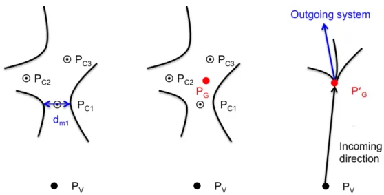
Figure 3: Schematic view of NI vertex reconstruction: (left) a cluster of PC positions (PC1, PC2,
and PC3) with the distance of closest approach dm (labeled dm1), shown for PC1; (center) the
algorithm uses the three PCpoints to identify an aggregate position PG; (right) after refitting the
track helices, the best vertex PG0 is found with indicated incoming direction from the primary vertex position, PV, and outgoing system. Black curves correspond to reconstructed charged
particle tracks.
Tracks considered for NI reconstruction benefit from all ten iterations and are required to have pT > 200 MeV to reduce the number of misreconstructed NIs. They are classified into three
categories according to their position relative to the NI vertex:
• Incoming tracks: we require d0<0.2 cm, and at least three hits, with at most one hit
after the NI vertex.
• Outgoing tracks: we require d0>0.2 cm, at least six hits, with at most one hit before
the NI vertex, and nlost<10.
• Merged tracks: we require d0<0.2 cm, at least four hits, with at least two hits before,
and two after the NI vertex, and nlost <10.
For an NI in the strip detector, the incoming charged particles may be reconstructed as short tracks seeded from pixel detector triplets or pairs of hits. For an NI in the pixel detector the incoming charged particle leaves too few hits to be reconstructed. It can happen, though, that the hits from the incoming charged particle are assigned by the tracking algorithm to an out-going track that is much longer. In that case, a merged track is obtained. The tracking of the outgoing charged particles typically uses strip-only or mixed pixel-strip detector seeding. Fi-nally, in NI cases where most of the momentum of the incoming charged hadron is transferred to an outgoing one, the trajectories of the incoming and outgoing tracks may be assigned by the tracking algorithm to a single merged track.
A vertex reconstructed from the list of selected tracks identifies the position of the NI. For each pair of tracks the points of closest approach are identified. The length of the segment connecting these two points provides the distance of closest approach, dm[20]. If dm<0.5 cm,
we consider the possibility that both tracks come from the same vertex. The center, PC, of
the segment is then considered as the best estimate of the position of this vertex. This step is sketched in Fig. 3 (left).
of vertex candidates. In practice, we start from the innermost PC (labeled PC1) with respect to
the primary vertex position, PV, and look for the presence of points within a cylinder of±5 cm
along the direction of the vector−−−→PVPC and 1 cm in radius. The dimensions of this cylinder are
defined to take into account the resolution of the track parameters. If several points are found, the closest to PC1 is selected, and the barycenter position (PG) between this point and PC1 is
calculated. The algorithm is iterated starting from PG. The search stops when no additional
points are found within the cylinder. This step is sketched in Fig. 3 (center). All points selected during the search are removed from the list of PCvalues and the algorithm is restarted.
Each PGwith its associated tracks is passed to the adaptive vertex fitter (AVF) [20], which refits
the helices of the tracks assuming a point close to PG as the common vertex. An example is
sketched in Fig. 3 (right). The AVF provides a list of vertex candidates with their best position estimates, PG0, as its output.
The set of outgoing tracks from a vertex candidate is referred to as the outgoing system. The Lorentz four-vectors of those tracks, assuming a pion mass for each track, define the kinematic properties of the outgoing system. The incoming or merged track is referred to as the incoming system. It provides the direction and kinematic properties of the impinging particle. In case no incoming or merged track is present, the vector−−−→PVPG0 defines the incoming direction.
This list of vertex candidates is filtered with the following quality criteria designed to select NI vertices and reject conversions, decays in flight, and misreconstructed NI vertices:
• At least three tracks are required, including incoming, merged, or outgoing tracks.
• An NI candidate with more than one incoming and/or merged track is rejected.
• The outgoing system must have an invariant mass of at least 1 GeV and pT >500 MeV.
• The angle between the incoming and outgoing directions shall not exceed 15◦.
• Vertex candidates located well inside the nominal beam pipe radius are removed since there is no material in that region.
With these criteria, 5.40 million events are found with at least one NI and these events yield a total of 5.71 million NIs.
The position resolution of the reconstructed NI vertices is estimated using the single-pion sim-ulation. The positions of the actual NI and its reconstruction are recorded and the differences are compared in different regions of the detector. Within the beam pipe, the typical resolution perpendicular to the direction of the particle’s propagation is of the order of 50 µm. The res-olution degrades at larger radius due to the smaller number of pixel detector hits included in the tracking. Within the pixel detector volume, the resolution is approximately 100 µm, and it increases to 200 µm within the pixel detector support tube. The perpendicular vertex position resolution is the main factor in determining how well the centers of the different structures can be located. The vertex position resolution along the direction of propagation of the incom-ing track is worse than in the perpendicular direction because the combinincom-ing of the individual track locations is less precise in this direction. The resolutions along the track direction are 300 µm within the beam pipe, 500 µm within the pixel detector, and 1000 µm within the pixel detector support tube. These resolutions are smaller than the element thicknesses in the dif-ferent structures under consideration and the impact on the uncertainties associated with the measurement procedure remains limited.
The purity of the NI sample depends on the region under consideration and the signal-over-background ratio is about 1.5, 0.5, and 8 for the beam pipe, BPIX detector inner shield, and pixel
7 BPIX detector support rails Pixel detector support tube BPIX detector longitudinal support BPIX detector outer shield Beam pipe BPIX detector inner shield BPIX detector layer 1, 2, and 3 TIB detector layer 1
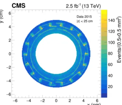
Figure 4: Hadrography of the tracking system in the x-y plane in the barrel region (|z| <25 cm). The density of NI vertices is indicated by the color scale. The signatures of the beam pipe, the BPIX detector with its support, and the first layer of the TIB detector can be observed above the background of misreconstructed NIs.
detector support tube, respectively. The misreconstruction rate decreases as track density de-creases and so it is smaller at higher radius. The misreconstruction rate for each measurement is estimated from data by looking at a region to the side of the structure under consideration, where no material is expected.
The “hadrography” in the x-y plane of the tracking system in the barrel region (|z| <25 cm) is provided in Fig. 4. The signatures of the beam pipe, the BPIX detector with its support, and the first layer of the TIB detector can be seen.
4
Analysis method
In this analysis we focus on the measurement of the positions of the inactive elements within the inner tracking system. All the inactive elements under consideration except for the sup-port rails have a cylindrical geometry with their axes being collinear to the beam axis. For all the structures but the support rails, the axis position is within a few millimeters of(0, 0), the origin of the CMS offline coordinate system, which is discussed in Section 7.1. By design, the thicknesses of the structures do not exceed a few millimeters to keep the amount of material within the inner tracking system to a minimum. These properties of the components under
consideration allow a significant simplification of the fitting technique. Instead of a complex fit of a 3D structure, we fit the parameters of a function in the x-y plane using shapes such as circles, half-circles, or ellipses.
The slight displacement of the structures’ axes with respect to the beam axis induces differences in the azimuthal hadron fluxes seen by different elements of the structure. We correct for that effect locally by reweighting events [8] using a geometric factor for each bin i, Fi, that accounts
for the small flux effect. To a first approximation we can write Fi = 1/r2i,bs, where rbs is the
radial distance calculated with respect to the average over the data-taking period of the beam spot position that was computed using the method from Ref. [20]. For the 2015 data-taking period, the average beam spot position in the transverse plane was xbs = 0.8 mm and ybs =
0.9 mm [22]. The beam spot position varied during the year by distances of less than 0.1 mm. The measurement of each cylindrical structure follows the same steps:
1. The NI vertices are selected within a ring of a few centimeters around the structure and a binned position distribution in i is made in the x-y plane. The chosen bin sizes are smaller than the thicknesses of the objects being studied, but large enough to allow for stable fitting procedures. The two-dimensional (2D) bin size in the x-y plane used for the beam pipe and BPIX detector inner shield measurements is 500×500 µm2. For the pixel detector support tube the bin size is 1700×1700 µm2, and for the BPIX detector support
rails a bin size of 800×800 µm2is used.
2. The resulting distribution is sliced into 40 regions in φ. The slices where additional struc-tures such as cooling pipes or collars, are visible near the main structure are rejected from the analysis.
3. In each slice, the 2D distribution is projected along the φ coordinate and the distribution of ρi(x0, y0)values is considered, where ρi(x0, y0) =
√
(xi−x0)2+ (yi−y0)2 is the
ra-dial position of the center of bin i in the relative coordinates of the structure, with origin
(x0, y0). The signal region is defined using ρmin and ρmax values chosen around the
ex-pected position of the structure. The combinatorial background is estimated using signal sidebands in ρi(x0, y0), which are fit by an exponential function, yielding a value Bi of
background events under the signal in the x-y plane for each bin i. 4. A χ2is defined for a circular shape:
χ2 =
∑
i:ρmin<ρi(x0,y0)<ρmax
max[0,(Ni−Bi−nσ √
Bi)]Fi/Fref(ρi(x0, y0) −R)2
σNI2 , (1)
where σNI = 100 µm is the typical NI vertex resolution, Ni is the number of events in
bin i, nσ is the number of standard deviations above the nominal background, and R is
the radius of the structure. In the case of an ellipse, R becomes dependent on xi and yi
through a relation parametrized by the semi-minor axis (Rx) and semi-major axis (Ry).
The correction factor Fi/Fref is defined to mitigate the small differences in hadron flux
between bins. To keep this factor as close as possible to 1, we take Fref to be the value of
the flux at the expected radius R around the beam spot position. During the minimization procedure we do not recalculate Fref. The overall impact of the flux factor on the final result is small.
5. We subtract the mean background plus twice the expected background uncertainty (using nσ=2) to maximize the signal purity and improve the visibility of the structures.
9
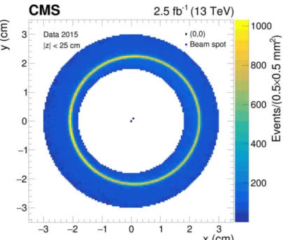
Figure 5: The beam pipe region viewed in the x-y plane for|z| < 25 cm before background subtraction. The density of NI vertices is indicated by the color scale. (0, 0) is the origin of the CMS offline coordinate system, which is discussed in Section 7.1. The blue point in the center of the distribution corresponds to the average beam spot position of xbs = 0.8 mm and ybs=0.9 mm in 2015.
6. A minimization of the χ2 is subsequently performed with R, x0, and y0, as free
parame-ters.
5
Measurements of pixel detector positions
5.1 Measurement of the beam pipe position
The density of NI vertices before background subtraction, reconstructed in the BPIX detector (|z| < 25 cm) in the region of the beam pipe ring, projected onto the x-y plane, is shown in Fig. 5. The section of the pipe observed in the figure is machined as a thin beryllium cylinder, 0.8 mm thick. The pipe is maintained by collars located at z = ±1.5 m, which are outside of the region that is investigated by this analysis. The structure is therefore modeled by a simple circle in the x-y plane. The combinatorial background appears in blue in the figure. Since the axis of the pipe is shifted by approximately 1 mm with respect to the coordinate system, we consider the whole region between ρmin=2.0 and ρmax=2.4 cm for the fit.
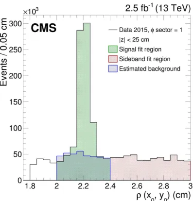
An example of a φ slice is shown in Fig. 6. We clearly see a peak at around ρ(x0, y0) =2.25 cm
that represents the location of the beam pipe. The combinatorial background under the peak is estimated from the right sideband defined by 2.4<ρ(x0, y0) <3.0 cm. An exponential function
is fitted to the sideband region and extrapolated into the signal region.
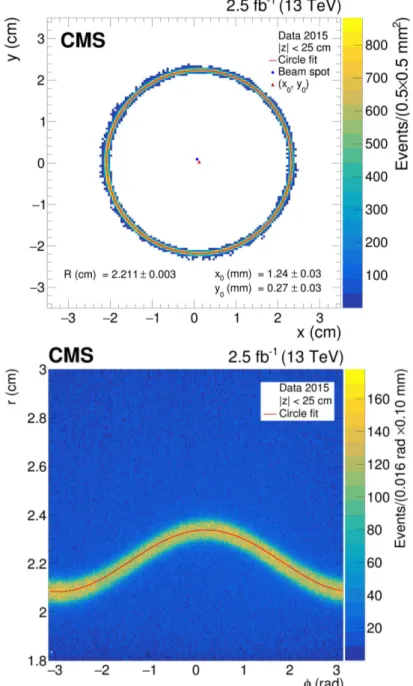
In Fig. 7, the fit results for a circle of radius R and center(x0, y0)are shown in the x-y plane
(upper), and r-φ coordinates (lower). The radius is measured with a precision of 30 µm, well below the thickness of the beam pipe. The radius measurement matches exactly the design value of the beam pipe, which is 22.1 mm [10]. The center of the beam pipe is shifted by 1.24 mm in x and 0.27 mm in y. The effect of this shift is visible in the sinusoidal modulation of the r-φ distribution, which is well modeled by the fit.
Figure 6: The density of NI vertices versus ρ(x0, y0)for a φ slice of the beam pipe located near
φ = 0 (black line) for |z| < 25 cm before background subtraction. The green hatched area
corresponds to the signal region, the red hatched area corresponds to the sideband region used to fit the background, and the blue hatched area corresponds to the estimated background in the signal region.
5.1 Measurement of the beam pipe position 11
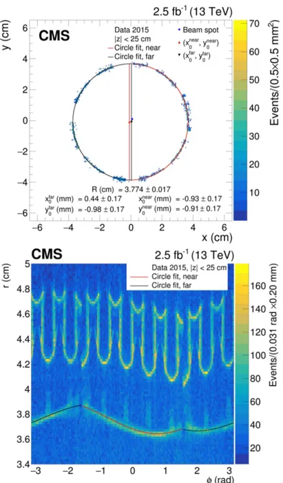
Figure 7: The beam pipe region with the fitted values for a circle of radius R and center(x0, y0)
for|z| < 25 cm. The x-y plane after background subtraction (upper), and the r-φ coordinates before background subtraction (lower), are shown. The density of NI vertices is indicated by the color scale. The red line shows the fitted circle. The blue point in the center of the x-y plane corresponds to the average beam spot position of xbs=0.8 mm and ybs=0.9 mm in 2015.
Figure 8: The BPIX detector inner shield region viewed in the x-y plane for|z| <25 cm before background subtraction and removal of the φ regions with additional structures. The density of NI vertices is indicated by the color scale. The inner shield itself is the visible circle of radius r = 3.8 cm. Modules in the first BPIX detector layer are visible at larger radius. The small bumps that can be seen around the shield correspond to cables connected to the first BPIX detector layer.
5.2 Measurement of the BPIX detector inner shield position
Figure 8 shows the density of reconstructed NI vertices in the region of the BPIX detector inner shield for |z| < 25 cm as projected onto the x-y plane. The inner shield can be identified at around r = 3.8 cm and protects the sensitive modules of the first BPIX detector layer visible in the region around r = 4 cm. The small bumps around the shield that are visible in Fig. 8 correspond to the cables connected to the first BPIX detector layer. The twelve φ sectors that contain the cables are removed from the fit described below.
The background for the remaining φ sectors is estimated from the left sideband defined by 3.00 < ρ(x0, y0) < 3.55 cm. This region between the beam pipe and the BPIX detector inner
shield is empty of any structure, while the region between the inner shield and first BPIX de-tector layer is very small and occupied by cables. The signal-over-background ratio for the BPIX detector inner shield is less favorable than for the beam pipe because the shield has a smaller amount of material.
In Fig. 9, the result of the fit to the BPIX detector inner shield with two half-circles is shown in the x-y plane (upper), and r-φ coordinates (lower). The radii of the halves are assumed to be equal and represented by the parameter R. The possibilities that the radii could be different and that we have two half-ellipses instead of circles were tested and represent the dominant systematic uncertainty, which amounts to 170 µm. The centers of each half-circle, (xfar0 , yfar0 ) and (xnear0 , ynear0 ), are determined from the fit. The fit values for yfar0 and ynear0 show that the halves are vertically aligned to within 100 µm. The geometric shapes of the two half-circles used in the fit overlap, as seen in Fig. 9 (upper). However, each half of the actual BPIX detector inner shield spans less than a half-circle in arc length, resulting in a small gap between the halves that can be seen in Figs. 8 and 9 (lower).
5.2 Measurement of the BPIX detector inner shield position 13
Figure 9: The BPIX detector inner shield with the fitted values for two half-circles of common radius R and centers (xfar0 , yfar0 ) and (x0near, ynear0 ) for|z| <25 cm. The x-y plane after background subtraction (upper), and the r-φ coordinates before background subtraction (lower), are shown. The density of NI vertices is indicated by the color scale. The red and black lines at around r =3.8 cm show the fitted half-circles on the far and near sides, respectively. The blue point at the center of the x-y plane corresponds to the average beam spot position of xbs=0.8 mm and
ybs = 0.9 mm in 2015. Modules in the first BPIX detector layer are visible in (lower) at larger
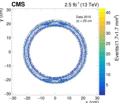
Figure 10: The region of the pixel detector support tube viewed in the x-y plane for|z| <25 cm before background subtraction and removal of the φ regions with additional structures. The density of NI vertices is indicated by the color scale. Two circular structures are visible. The circle with the smaller radius corresponds to the BPIX detector outer shield, while the one with the larger radius is the pixel detector support tube (also visible in Fig. 4).
5.3 Measurements of the positions of the pixel detector support tube and the BPIX detector support rails
The density of NI vertices, reconstructed in the barrel tracking detector (|z| < 25 cm), in the region of the pixel detector support tube, projected onto the x-y plane, is shown in Fig. 10. The BPIX detector is placed within the cylinder of the pixel detector support tube using the top and bottom rails visible at y ≈ ±19 cm. The region around the rails (twelve φ sectors) is removed from the fitting procedure for the pixel detector support tube.
When the pixel detector support tube was manufactured, it was circular, but it was deformed into an ellipse under its own weight after installation. The pixel detector support tube was fitted with an ellipse because of this deformation, and a difference of 1.0 mm is seen between the two semi-axes. In Fig. 11, the result of the fit to the pixel detector support tube is shown in the x-y plane (upper), and r-φ coordinates (lower). The semi-minor axis appears to be aligned with the x axis and the semi-major axis with the y axis. The position of the center of the pixel detector support tube is shifted by a few millimeters with respect to the coordinate system. The method used to measure the positions of the BPIX detector support rails is different than for the other inactive elements since the rails are more complex structures to model. The rails are mounted on support structures that are aligned with the x axis, therefore we can identify the y coordinate (top rail y and bottom rail y) of this support structure. In practice we define top and bottom rail y as the inner coordinate of the support structure, estimated by finding the position with the maximum y derivative in Fig. 12. The measurement is performed separately for the y < 0 and y > 0 sides. Since the support structure is very thin, it is included in a single bin of width 800 µm. The uncertainty for a uniform/flat distribution is 1/√12 of the bin size, i.e., 0.02 cm. This uncertainty includes effects from the fitting procedure and from small structures within the rails. The results are shown in Fig. 12 for the combined tracking
5.3 Measurements of the positions of the pixel detector support tube and the BPIX detector support
rails 15
Figure 11: The pixel detector support tube with the fitted values for an ellipse with semi-minor axis Rx, semi-major axis Ry, and center(x0, y0)for|z| <25 cm. The x-y plane after background
subtraction (upper), and the r-φ coordinates before background subtraction (lower), are shown. The density of NI vertices is indicated by the color scale. The red line shows the fitted ellipse. The blue point in the center of the x-y plane corresponds to the average beam spot position of xbs=0.8 mm and ybs=0.9 mm in 2015.
Figure 12: The BPIX detector support rails after background subtraction in the x-y plane for the combined tracking detector barrel and endcap regions. Horizontal red lines correspond to the fit of the BPIX detector support rails. The density of NI vertices is indicated by the color scale. detector barrel and endcap regions. We also performed separate measurements for the barrel and endcap regions, and the results were consistent with those obtained from the combined regions.
5.4 Results
Table 1 summarizes the results of the fits. The values of the parameters are tabulated for the fits to the beam pipe with a circle, the BPIX detector inner shield with two half-circles, and the pixel detector support tube with an ellipse. Only systematic uncertainties are provided since the statistical uncertainties are negligible (below 10 µm). Table 2 summarizes the final results where the BPIX detector support rails were fitted with a horizontal line. As an estimate of the systematic uncertainty we take half the bin width in y; the statistical uncertainties are once again negligible.
Table 1: Results of the fit to the beam pipe with a circle, the BPIX detector inner shield with two half-circles, and the pixel detector support tube with an ellipse. Only systematic uncertainties are provided since the statistical uncertainties are negligible.
Object R (cm) x0(mm) y0(mm)
Beam pipe 2.211±0.003 1.24±0.03 0.27±0.03
BPIX detector inner shield, far 3.774±0.017 0.44±0.17 −0.98±0.17 BPIX detector inner shield, near 3.774±0.017 −0.93±0.17 −0.91±0.17 Pixel detector support tube Rx: 21.703±0.007 −0.75±0.07 −3.15±0.07
Ry: 21.803±0.007
6
Systematic uncertainties
The precision of the measurements presented in Table 1 is determined by the systematic uncer-tainties. These uncertainties are associated with the procedures for the background subtraction,
17
Table 2: Results of the fitted y coordinate of the bottom and top BPIX detector support rails with a horizontal line. Only systematic uncertainties are provided since the statistical uncertainties are negligible.
Bottom rail y (cm) Top rail y (cm)
−19.72±0.02 19.08±0.02
the shape assumptions, parameter fitting, and NI vertex reconstruction.
Table 3: Systematic uncertainties in the position and radius measurements of three inactive detector elements.
Source of systematic uncertainty Beam pipe BPIX detector Pixel detector (mm) inner shield (mm) support tube (mm)
Background shape 0.02 0.02 0.04
variation
Background subtraction <0.01 0.06 0.01
Average background <0.01 0.02 <0.01
in three neighbor φ bins
Structure shape <0.01 0.07 (position) —
variation 0.14 (Rnear,Rfar)
Fit procedure 0.01 0.01 0.04
Vertex reconstruction resolution 0.01 0.01 0.04
Total 0.03 0.17 0.07
Uncertainties arising from the subtraction and estimation of the background are determined by varying the shape and normalization of the background, and refitting the resulting signal. As a cross-check, instead of using an exponential fit, a simple horizontal line is fit in the sideband region and extrapolated into the signal region to determine the combinatorial background un-der the signal peak. The largest difference seen in the fitted values for each structure is taken as the systematic uncertainty due to the background shape. The normalization of the background was also varied. The number of background events in each bin was varied by two standard deviations in the statistical uncertainty and the resulting signal was refitted. The maximum difference in the fitted values is taken as the systematic uncertainty associated with the esti-mated size of the background subtraction. A third background variation was performed by using the background estimated from neighboring φ bins. Again, the difference in fitted values is taken as a systematic uncertainty. The uncertainties from these variations on the background are listed in Table 3. The combined effect of these three sources does not exceed 60 µm.
The uncertainties in the measurements that were introduced by the assumptions made about the shapes of the beam pipe and BPIX detector inner shield are also estimated by refitting the data using different shapes. The uncertainties in the shapes of the beam pipe and BPIX detector inner shield are estimated by fitting the beam pipe with an ellipse, instead of a circle, and the BPIX detector inner shield with two half-ellipses, instead of two half-circles. In the case of the beam pipe, it is observed that the two semi-axes of the ellipse are equal to within 10 µm, which supports the use of a circular shape, and this difference is added to the systematic uncertainty of the radius measurement. The value of Rx was fixed for the BPIX detector inner shield fits
to the half-ellipse, because otherwise the fit was not stable. The results from the ellipse and half-ellipse fits were compared with the results from the circle and half-circle fits. The largest difference was taken as the systematic uncertainty from the shape of the structure. The pixel detector support tube is already modeled with an ellipse, and therefore no extra systematic uncertainty is assigned to the modeling of its shape. The systematic uncertainties determined
by varying the assumed shapes of the structures are listed in Table 3.
The systematic uncertainties associated with the fit procedure are determined using pseudo-data where the shapes and positions of the objects are fixed from the experimentally measured values. Uncertainties for the fits to a circular shape are measured by generating a beam pipe centered at (0, 0), a beam pipe centered at the measured (x, y), a BPIX detector inner shield generated with the values measured from the near side, and a BPIX detector inner shield gen-erated with the values measured from the far side. The largest difference between the input parameters and the fit results was taken as the systematic uncertainty for the circle fit. The systematic uncertainty from the fit to an elliptical shape was determined similarly. Two pixel detector support tubes were generated. One was centered at(0, 0)with the semi-axes similar to the measured values, and the other was centered at the measured center of the pixel detec-tor support tube with semi-axes similar to the measured values. The uncertainties found from fitting the simulated data are listed in Table 3 in the “Fit procedure” row.
Another source of systematic uncertainty comes from the reconstruction of the secondary ver-tex position for the NI. The finite position resolution of the reconstructed vertices and the fitting procedure itself may introduce biases in the position measurements. The effects of these po-tential biases are estimated by measuring the structure properties in MC simulations based on single pions generated where a cylindrical model is assumed for the beam pipe, BPIX detector inner shield and pixel detector support tubes centered on the beam axis. Pions with momenta of 10 and 100 GeV are simulated. The simulated beam pipe, BPIX detector inner shield, and pixel detector support tube are centered at(0, 0). The largest deviations from (0, 0)in the fits are taken as the systematic uncertainties, and are presented in Table 3 in the “Vertex reconstruc-tion resolureconstruc-tion” row.
The systematic uncertainty in the position measurements for the BPIX detector support rails is conservatively estimated to be 1/√12 of the bin size.
During the 2015 data taking, CMS had cooling problems with its magnet, resulting in the mag-net being cycled on and off several times. Since the changes in magmag-netic field could potentially affect the position of the beam pipe, the data were split into two halves chronologically to see if the position in the later data differed from that in the earlier data. Within the measurement uncertainties, no change in position was observed.
7
Comparison with technical surveys
After the installation of the new CMS central beam pipe [23] during the 2013–2015 LHC shut-down, a number of measurements were taken in order to better understand the position and stability under different supporting configurations of the central beam pipe itself and later also of the BPIX detector. The pixel detector support tube was not surveyed at this time because NI measurements had shown no motion of it with respect to earlier surveys and it is not possible to adjust its position in any case.
7.1 CMS survey coordinate system
The CMS coordinate system used by the surveyors is the same as that described in Section 2. The local geometry of the CMS cavern is a local transformation from the global geometry of the LHC. The coordinate system used for offline analysis in CMS is based on a 3D best fit reconstruction from high pT tracks coming from the interaction region of the TOB centroid.
The reconstructed TOB centroid defines the CMS detector central axis and, based on measure-ments taken by the surveyors at CMS after the installation of the tracking system in 2009 in the
7.2 Central beam pipe 19
CMS coordinate system, is made to coincide with the latter in the offline code via simple rigid translations and rotations. The two coordinate systems (CMS offline system and CMS coordi-nate system) should then coincide within the uncertainties that are domicoordi-nated by the surveyors measurements. The systematic uncertainty is estimated to be±0.75 mm and it should be added to any other quoted uncertainties when comparing results obtained within the two systems.
7.2 Central beam pipe
The CMS central beam pipe spans the central detector region over 6.2 m and is held vertically and horizontally by metal wires attached to collars positioned at±1.6 m from the center and at the two extremities (±3.1 m) by flanges connected to the endcap sections of the beam pipe. Measurements of the position of the beam pipe were taken using a theodolite and measuring four points for each collar and flange. A best fit to a circle gives the position of the center of the beam pipe in the four positions along the z axis. The accuracy of this measurement is estimated to be±0.5 mm. Table 4 summarizes the results of the measurements of the CMS central beam pipe on January 12, 2015 after the re-installation of the original pixel detector (both barrel and endcaps parts) and with all supports in their final configuration.
Table 4: Results from the survey of the CMS central beam pipe positions on January 12, 2015.
Support x ( mm) y ( mm) z ( mm)
Flange+z (+3.1 m) 0.2 0.2 3131.7 Collar+z (+1.6 m) 0.8 0.2 — Collar−z (−1.6 m) 0.7 0.1 — Flange−z (−3.1 m) −0.8 0.2 −3136.9
Although these results should be directly compared with the NI measurements taken shortly thereafter during 2015 data taking, there are several considerations to be made, potentially leading to a somewhat different position of the beam pipe during data taking:
• The CMS endcaps needed to be closed, and in the process, various beam pipe sup-ports are temporarily removed and exchanged.
• The magnetic field was turned on, compressing the endcaps inside the solenoid toward the interaction point (hence the need for various supports along the beam pipe).
• Vacuum was created inside the beam pipe before the beam can circulate.
• The ambient temperature in the tracking system and central beam pipe volume went down to around 0◦C during data taking.
Notwithstanding these differences, the survey coordinates of the center of the beam pipe are compatible with the NI measurements. The x and y coordinates in Table 1 for|z| <25 cm agree within uncertainties with the inner beam pipe (collar) positions given in Table 4.
7.3 BPIX detector
In order to be able to measure the position of the BPIX detector right after installation, optical targets were glued onto the end flanges of the detector, which are visible from outside the pixel detector support tube using a theodolite positioned on the pixel detector installation platform at each end. The BPIX detector is divided into two separate parts labeled far and near as discussed in Section 2. The detector itself spans the interaction region over about 50 cm in the z
direction, but the services, running along the outside surface of the pixel detector supply tube, extend to the end of the pixel detector volume at z= ±3.0 m.
Three survey target points, indicated by the numbers 2001, 2002, and 2003, are visible in Fig. 2 (right): one survey mark and two mechanical flat screws were used to define the plane of the end flange of the detector, and the positions are measured using photogrammetry tech-niques in the laboratory before installation. The three points on each of the four end flanges of the detector (near+z, near−z, far+z, and far−z) were then referenced to the center axis of the BPIX detector with an estimated accuracy of±0.2 mm. The detector was installed on December 11, 2014 and its position measured with the theodolite. The three points at each end define a plane and a center, and the two planes combined define a center line in 3D space. Each side (far and near) is treated independently yielding two center lines in 3D space, one extrapolated from measurements of the far side and one from measurements of the near side. The accuracy of the two extrapolated center lines is estimated to be±1.0 mm. From these measurements the survey determined that the overall detector center is low by 1.1 mm (y= −1.1 mm for both the far and near halves), in good agreement with the y0results shown in Table 1. In the x direction,
the average of the far and near center positions is−0.7 mm in the survey, which agrees within the uncertainties with the average value of−0.2 mm from the NI measurements.
8
Summary
Nuclear interactions have a reputation of being undesirable events that degrade the quality of the reconstruction of charged and neutral hadrons. In this analysis, it has been demonstrated that they can be used to produce a high-precision map of the material inside the tracking sys-tem. Such maps can be useful for validating detector simulations and identifying any shifts in detector elements during operation.
Using a data set that corresponds to an integrated luminosity of 2.5 fb−1 of proton-proton col-lisions at a center-of-mass energy of 13 TeV, a large sample of secondary hadronic interactions was collected. After background subtraction, the positions of the secondary vertices were used to determine the locations of inactive elements with a precision of the order of 100 µm. The po-sitions of the beam pipe and the inner tracking system structures (pixel detector support tube, and BPIX inner shield and support rails) were determined with a precision that depends on the structure under study. No significant position bias was identified through the technique, and statistical uncertainties were negligible. The positions of the structures under consideration were probed with a precision better than the typical installation tolerances and are found to be compatible with previous survey measurements.
Acknowledgments
We congratulate our colleagues in the CERN accelerator departments for the excellent perfor-mance of the LHC and thank the technical and administrative staffs at CERN and at other CMS institutes for their contributions to the success of the CMS effort. In addition, we grate-fully acknowledge the computing centers and personnel of the Worldwide LHC Computing Grid for delivering so effectively the computing infrastructure essential to our analyses. Fi-nally, we acknowledge the enduring support for the construction and operation of the LHC and the CMS detector provided by the following funding agencies: BMWFW and FWF (Aus-tria); FNRS and FWO (Belgium); CNPq, CAPES, FAPERJ, FAPERGS, and FAPESP (Brazil); MES (Bulgaria); CERN; CAS, MoST, and NSFC (China); COLCIENCIAS (Colombia); MSES and CSF (Croatia); RPF (Cyprus); SENESCYT (Ecuador); MoER, ERC IUT, and ERDF (Estonia);
References 21
Academy of Finland, MEC, and HIP (Finland); CEA and CNRS/IN2P3 (France); BMBF, DFG, and HGF (Germany); GSRT (Greece); NKFIA (Hungary); DAE and DST (India); IPM (Iran); SFI (Ireland); INFN (Italy); MSIP and NRF (Republic of Korea); LAS (Lithuania); MOE and UM (Malaysia); BUAP, CINVESTAV, CONACYT, LNS, SEP, and UASLP-FAI (Mexico); MOS (Mon-tenegro); MBIE (New Zealand); PAEC (Pakistan); MSHE and NSC (Poland); FCT (Portugal); JINR (Dubna); MON, RosAtom, RAS, RFBR, and NRC KI (Russia); MESTD (Serbia); SEIDI, CPAN, PCTI, and FEDER (Spain); MOSTR (Sri Lanka); Swiss Funding Agencies (Switzerland); MST (Taipei); ThEPCenter, IPST, STAR, and NSTDA (Thailand); TUBITAK and TAEK (Turkey); NASU and SFFR (Ukraine); STFC (United Kingdom); DOE and NSF (USA). Individuals have received support from the Marie-Curie program and the European Research Council and Hori-zon 2020 Grant, contract No. 675440 (European Union); the Leventis Foundation; the A. P. Sloan Foundation; the Alexander von Humboldt Foundation; the Belgian Federal Science Policy Of-fice; the Fonds pour la Formation `a la Recherche dans l’Industrie et dans l’Agriculture (FRIA-Belgium); the Agentschap voor Innovatie door Wetenschap en Technologie (IWT-(FRIA-Belgium); the F.R.S.-FNRS and FWO (Belgium) under the “Excellence of Science - EOS” - be.h project n. 30820817; the Ministry of Education, Youth and Sports (MEYS) of the Czech Republic; the Lend ¨ulet (“Momentum”) Programme and the J´anos Bolyai Research Scholarship of the Hun-garian Academy of Sciences, the New National Excellence Program ´UNKP, the NKFIA research grants 123842, 123959, 124845, 124850 and 125105 (Hungary); the Council of Science and In-dustrial Research, India; the HOMING PLUS program of the Foundation for Polish Science, cofinanced from European Union, Regional Development Fund, the Mobility Plus program of the Ministry of Science and Higher Education, the National Science Center (Poland), contracts Harmonia 2014/14/M/ST2/00428, Opus 2014/13/B/ST2/02543, 2014/15/B/ST2/03998, and 2015/19/B/ST2/02861, Sonata-bis 2012/07/E/ST2/01406; the National Priorities Research Program by Qatar National Research Fund; the Programa Estatal de Fomento de la Investi-gaci ´on Cient´ıfica y T´ecnica de Excelencia Mar´ıa de Maeztu, grant MDM-2015-0509 and the Programa Severo Ochoa del Principado de Asturias; the Thalis and Aristeia programs cofi-nanced by EU-ESF and the Greek NSRF; the Rachadapisek Sompot Fund for Postdoctoral Fel-lowship, Chulalongkorn University and the Chulalongkorn Academic into Its 2nd Century Project Advancement Project (Thailand); the Welch Foundation, contract C-1845; and the We-ston Havens Foundation (USA); the Hellenic Foundation for Research and Innovation, HFRI; the Fondazione Ing. Aldo Gini.
References
[1] CMS Collaboration, “The CMS experiment at the CERN LHC”, JINST 3 (2008) S08004, doi:10.1088/1748-0221/3/08/S08004.
[2] CMS Collaboration, “Search for long-lived charged particles in proton-proton collisions at√s=13 TeV”, Phys. Rev. D 94 (2016) 112004,
doi:10.1103/PhysRevD.94.112004, arXiv:1609.08382.
[3] CMS Collaboration, “Search for new long-lived particles at√s=13 TeV”, Phys. Lett. B 780(2018) 432, doi:10.1016/j.physletb.2018.03.019, arXiv:1711.09120. [4] CMS Collaboration, “Identification of heavy-flavour jets with the CMS detector in pp
collisions at 13 TeV”, JINST 13 (2018) P05011,
doi:10.1088/1748-0221/13/05/P05011, arXiv:1712.07158.
[5] GEANT4 Collaboration, “GEANT4—a simulation toolkit”, Nucl. Instrum. Meth. A 506 (2003) 250, doi:10.1016/S0168-9002(03)01368-8.
[6] J. Allison et al., “GEANT4 developments and applications”, IEEE Trans. Nucl. Sci. 53 (2006) 270, doi:10.1109/TNS.2006.869826.
[7] CMS Collaboration, “Altered scenarios of the CMS tracker material for systematic uncertainties studies”, Technical Report CMS-NOTE-2010-010, CERN, 2010.
[8] CMS Collaboration, “Studies of tracker material”, CMS Physics Analysis Summary CMS-PAS-TRK-10-003, CERN, 2010.
[9] CMS Collaboration, “Performance of photon reconstruction and identification with the CMS detector in proton-proton collisions at√s=8 TeV”, JINST 10 (2015) P08010, doi:10.1088/1748-0221/10/08/P08010, arXiv:1502.02702.
[10] CMS Collaboration, “CMS technical design report for the pixel detector upgrade”, technical report, CERN, 2012. doi:10.2172/1151650.
[11] ATLAS Collaboration, “A study of the material in the ATLAS inner detector using secondary hadronic interactions”, JINST 7 (2012) P01013,
doi:10.1088/1748-0221/7/01/P01013, arXiv:1110.6191.
[12] ATLAS Collaboration, “A measurement of material in the ATLAS tracker using secondary hadronic interactions in 7 TeV pp collisions”, JINST 11 (2016) P11020, doi:10.1088/1748-0221/11/11/P11020, arXiv:1609.04305.
[13] ATLAS Collaboration, “Study of the material of the ATLAS inner detector for Run 2 of the LHC”, JINST 12 (2017) P12009, doi:10.1088/1748-0221/12/12/P12009, arXiv:1707.02826.
[14] CMS Collaboration, “Alignment of the CMS tracker with LHC and cosmic ray data”, JINST 9 (2014) P06009, doi:10.1088/1748-0221/9/06/P06009,
arXiv:1403.2286.
[15] T. Sj ¨ostrand, S. Mrenna, and P. Z. Skands, “A brief introduction toPYTHIA8.1”, Comput. Phys. Commun. 178 (2008) 852, doi:10.1016/j.cpc.2008.01.036,
arXiv:0710.3820.
[16] T. Sj ¨ostrand et al., “An introduction toPYTHIA8.2”, Comput. Phys. Commun. 191 (2015) 159, doi:10.1016/j.cpc.2015.01.024, arXiv:1410.3012.
[17] CMS Collaboration, “Event generator tunes obtained from underlying event and multiparton scattering measurements”, Eur. Phys. J. C 76 (2016) 155,
doi:10.1140/epjc/s10052-016-3988-x, arXiv:1512.00815. [18] CMS Collaboration, “The CMS trigger system”, JINST 12 (2017) P01020,
doi:10.1088/1748-0221/12/01/P01020, arXiv:1609.02366.
[19] CMS Tracker Collaboration, R. Ranieri, “The simulation of the CMS silicon tracker”, in Proceedings, 2007 IEEE Nuclear Science Symposium and Medical Imaging Conference
(NSS/MIC): Honolulu, Hawaii, p. 2434. 2007. doi:10.1109/NSSMIC.2007.4436649. [20] CMS Collaboration, “Description and performance of track and primary-vertex
reconstruction with the CMS tracker”, JINST 9 (2014) P10009, doi:10.1088/1748-0221/9/10/P10009, arXiv:1405.6569.
References 23
[21] CMS Collaboration, “Particle-flow reconstruction and global event description with the CMS detector”, JINST 12 (2017) P10003, doi:10.1088/1748-0221/12/10/P10003, arXiv:1706.04965.
[22] CMS Collaboration, “Tracking POG plot results on 2015 data”, Technical Report CMS-DP-2016-012, CERN, 2016.
[23] M. Gallilee et al., “LHC detector vacuum system consolidation for long shutdown 1 (LS1) in 2013-2014”, in Proceedings, 3rd International Conference on Particle accelerator (IPAC 2012): New Orleans, USA, p. 2555. 2012.
25
A
The CMS Collaboration
Yerevan Physics Institute, Yerevan, Armenia A.M. Sirunyan, A. Tumasyan
Institut f ¨ur Hochenergiephysik, Wien, Austria
W. Adam, F. Ambrogi, E. Asilar, T. Bergauer, J. Brandstetter, E. Brondolin, M. Dragicevic, J. Er ¨o, A. Escalante Del Valle, M. Flechl, R. Fr ¨uhwirth1, V.M. Ghete, J. Grossmann, J. Hrubec, M. Jeitler1, A. K ¨onig, N. Krammer, I. Kr¨atschmer, D. Liko, T. Madlener, I. Mikulec, N. Rad,
H. Rohringer, J. Schieck1, R. Sch ¨ofbeck, M. Spanring, D. Spitzbart, H. Steininger, A. Taurok, W. Waltenberger, J. Wittmann, C.-E. Wulz1, M. Zarucki
Institute for Nuclear Problems, Minsk, Belarus V. Chekhovsky, V. Mossolov, J. Suarez Gonzalez Universiteit Antwerpen, Antwerpen, Belgium
W. Beaumont, E.A. De Wolf, D. Di Croce, X. Janssen, J. Lauwers, M. Pieters, M. Van De Klun-dert, H. Van Haevermaet, P. Van Mechelen, N. Van Remortel
Vrije Universiteit Brussel, Brussel, Belgium
S. Abu Zeid, F. Blekman, E.S. Bols, J. D’Hondt, I. De Bruyn, J. De Clercq, K. Deroover, G. Flouris, D. Lontkovskyi, S. Lowette, I. Marchesini, S. Moortgat, L. Moreels, Q. Python, K. Skovpen, S. Tavernier, W. Van Doninck, P. Van Mulders, I. Van Parijs
Universit´e Libre de Bruxelles, Bruxelles, Belgium
Y. Allard, D. Beghin, B. Bilin, H. Brun, B. Clerbaux, G. De Lentdecker, H. Delannoy, B. Dorney, G. Fasanella, L. Favart, R. Goldouzian, A. Grebenyuk, A.K. Kalsi, T. Lenzi, J. Luetic, L. Moureaux, N. Postiau, Z. Song, E. Starling, C. Vander Velde, P. Vanlaer, D. Vannerom, Q. Wang
Ghent University, Ghent, Belgium
T. Cornelis, D. Dobur, A. Fagot, M. Gul, I. Khvastunov2, D. Poyraz, C. Roskas, D. Trocino,
M. Tytgat, W. Verbeke, B. Vermassen, M. Vit, N. Zaganidis
Universit´e Catholique de Louvain, Louvain-la-Neuve, Belgium
H. Bakhshiansohi, O. Bondu, S. Brochet, G. Bruno, C. Caputo, A. Caudron, P. David, S. De Visscher, C. Delaere, M. Delcourt, B. Francois, A. Giammanco, G. Krintiras, V. Lemaitre, A. Magitteri, A. Mertens, D. Michotte, M. Musich, K. Piotrzkowski, L. Quertenmont, A. Saggio, N. Szilasi, M. Vidal Marono, S. Wertz, J. Zobec
Universit´e de Mons, Mons, Belgium
N. Beliy, T. Caebergs, E. Daubie, G.H. Hammad
Centro Brasileiro de Pesquisas Fisicas, Rio de Janeiro, Brazil
F.L. Alves, G.A. Alves, L. Brito, G. Correia Silva, C. Hensel, A. Moraes, M.E. Pol, P. Rebello Teles Universidade do Estado do Rio de Janeiro, Rio de Janeiro, Brazil
E. Belchior Batista Das Chagas, W. Carvalho, J. Chinellato3, E. Coelho, E.M. Da Costa,
G.G. Da Silveira4, D. De Jesus Damiao, C. De Oliveira Martins, S. Fonseca De Souza, H. Malbouisson, D. Matos Figueiredo, M. Melo De Almeida, C. Mora Herrera, L. Mundim, H. Nogima, W.L. Prado Da Silva, L.J. Sanchez Rosas, A. Santoro, A. Sznajder, M. Thiel, E.J. Tonelli Manganote3, F. Torres Da Silva De Araujo, A. Vilela Pereira
Universidade Estadual Paulistaa, Universidade Federal do ABCb, S˜ao Paulo, Brazil
S. Ahujaa, C.A. Bernardesa, L. Calligarisa, T.R. Fernandez Perez Tomeia, E.M. Gregoresb, P.G. Mercadanteb, S.F. Novaesa, SandraS. Padulaa, D. Romero Abadb
Institute for Nuclear Research and Nuclear Energy, Bulgarian Academy of Sciences, Sofia, Bulgaria
A. Aleksandrov, R. Hadjiiska, P. Iaydjiev, A. Marinov, M. Misheva, M. Rodozov, M. Shopova, G. Sultanov
University of Sofia, Sofia, Bulgaria A. Dimitrov, L. Litov, B. Pavlov, P. Petkov Beihang University, Beijing, China W. Fang5, X. Gao5, L. Yuan
Institute of High Energy Physics, Beijing, China
M. Ahmad, J.G. Bian, G.M. Chen, H.S. Chen, M. Chen, Y. Chen, C.H. Jiang, D. Leggat, H. Liao, Z. Liu, F. Romeo, S.M. Shaheen, A. Spiezia, J. Tao, C. Wang, Z. Wang, E. Yazgan, H. Zhang, J. Zhao
State Key Laboratory of Nuclear Physics and Technology, Peking University, Beijing, China Y. Ban, G. Chen, J. Li, Q. Li, S. Liu, Y. Mao, S.J. Qian, D. Wang, Z. Xu
Tsinghua University, Beijing, China Y. Wang
Universidad de Los Andes, Bogota, Colombia
C. Avila, A. Cabrera, C.A. Carrillo Montoya, L.F. Chaparro Sierra, C. Florez, C.F. Gonz´alez Hern´andez, M.A. Segura Delgado
University of Split, Faculty of Electrical Engineering, Mechanical Engineering and Naval Architecture, Split, Croatia
B. Courbon, N. Godinovic, D. Lelas, I. Puljak, T. Sculac University of Split, Faculty of Science, Split, Croatia Z. Antunovic, M. Kovac
Institute Rudjer Boskovic, Zagreb, Croatia
V. Brigljevic, S. Ceci, D. Ferencek, K. Kadija, B. Mesic, A. Starodumov6, T. Susa University of Cyprus, Nicosia, Cyprus
M.W. Ather, A. Attikis, G. Mavromanolakis, J. Mousa, C. Nicolaou, F. Ptochos, P.A. Razis, H. Rykaczewski
Charles University, Prague, Czech Republic M. Finger7, M. Finger Jr.7
Escuela Politecnica Nacional, Quito, Ecuador E. Ayala
Universidad San Francisco de Quito, Quito, Ecuador E. Carrera Jarrin
Academy of Scientific Research and Technology of the Arab Republic of Egypt, Egyptian Network of High Energy Physics, Cairo, Egypt
27
National Institute of Chemical Physics and Biophysics, Tallinn, Estonia
I. Ahmed11, S. Bhowmik, A. Carvalho Antunes De Oliveira, R.K. Dewanjee, K. Ehataht, M. Kadastik, L. Perrini, M. Raidal, C. Veelken
Department of Physics, University of Helsinki, Helsinki, Finland P. Eerola, H. Kirschenmann, J. Pekkanen, M. Voutilainen
Helsinki Institute of Physics, Helsinki, Finland
J. Havukainen, J.K. Heikkil¨a, T. J¨arvinen, V. Karim¨aki, R. Kinnunen, T. Lamp´en, K. Lassila-Perini, S. Laurila, S. Lehti, T. Lind´en, P. Luukka, T. M¨aenp¨a¨a, H. Siikonen, E. Tuominen, J. Tuominiemi
Lappeenranta University of Technology, Lappeenranta, Finland T. Tuuva
IRFU, CEA, Universit´e Paris-Saclay, Gif-sur-Yvette, France
M. Besancon, F. Couderc, M. Dejardin, D. Denegri, J.L. Faure, F. Ferri, S. Ganjour, A. Givernaud, P. Gras, G. Hamel de Monchenault, P. Jarry, C. Leloup, E. Locci, J. Malcles, G. Negro, J. Rander, A. Rosowsky, M. ¨O. Sahin, M. Titov
Laboratoire Leprince-Ringuet, Ecole polytechnique, CNRS/IN2P3, Universit´e Paris-Saclay, Palaiseau, France
A. Abdulsalam12, C. Amendola, I. Antropov, F. Beaudette, P. Busson, C. Charlot, R. Granier de Cassagnac, I. Kucher, S. Lisniak, A. Lobanov, J. Martin Blanco, M. Nguyen, C. Ochando, G. Ortona, P. Pigard, R. Salerno, J.B. Sauvan, Y. Sirois, A.G. Stahl Leiton, Y. Yilmaz, A. Zabi, A. Zghiche
Universit´e de Strasbourg, CNRS, IPHC UMR 7178, Strasbourg, France
J.-L. Agram13, J. Andrea, D. Bloch, C. Bonnin, J.-M. Brom, E.C. Chabert, L. Charles, V. Cherepanov, C. Collard, E. Conte13, J.-C. Fontaine13, D. Gel´e, U. Goerlach, L. Gross, J. Hosselet, M. Jansov´a, A.-C. Le Bihan, N. Tonon, P. Van Hove
Centre de Calcul de l’Institut National de Physique Nucleaire et de Physique des Particules, CNRS/IN2P3, Villeurbanne, France
S. Gadrat
Universit´e de Lyon, Universit´e Claude Bernard Lyon 1, CNRS-IN2P3, Institut de Physique Nucl´eaire de Lyon, Villeurbanne, France
G. Baulieu, S. Beauceron, C. Bernet, G. Boudoul, L. Caponetto, N. Chanon, R. Chierici, D. Contardo, P. Depasse, T. Dupasquier, H. El Mamouni, J. Fay, L. Finco, G. Galbit, S. Gascon, M. Gouzevitch, G. Grenier, B. Ille, F. Lagarde, I.B. Laktineh, H. Lattaud, M. Lethuillier, N. Lumb, L. Mirabito, B. Nodari, A.L. Pequegnot, S. Perries, A. Popov14, V. Sordini, M. Vander Donckt,
S. Viret, S. Zhang
Georgian Technical University, Tbilisi, Georgia T. Toriashvili15
Tbilisi State University, Tbilisi, Georgia D. Lomidze
RWTH Aachen University, I. Physikalisches Institut, Aachen, Germany
C. Autermann, L. Feld, W. Karpinski, M.K. Kiesel, K. Klein, M. Lipinski, A. Ostapchuk, G. Pierschel, M. Preuten, M.P. Rauch, S. Schael, C. Schomakers, J. Schulz, G. Schwering, M. Teroerde, B. Wittmer, M. Wlochal, V. Zhukov14
RWTH Aachen University, III. Physikalisches Institut A, Aachen, Germany
A. Albert, D. Duchardt, M. Endres, M. Erdmann, S. Erdweg, T. Esch, R. Fischer, S. Ghosh, A. G ¨uth, T. Hebbeker, C. Heidemann, K. Hoepfner, S. Knutzen, L. Mastrolorenzo, M. Merschmeyer, A. Meyer, P. Millet, S. Mukherjee, T. Pook, M. Radziej, H. Reithler, M. Rieger, F. Scheuch, A. Schmidt, D. Teyssier, S. Th ¨uer
RWTH Aachen University, III. Physikalisches Institut B, Aachen, Germany
C. Dziwok, G. Fl ¨ugge, O. Hlushchenko, B. Kargoll, T. Kress, A. K ¨unsken, T. M ¨uller, A. Nehrkorn, A. Nowack, C. Pistone, O. Pooth, H. Sert, A. Stahl11, T. Ziemons
Deutsches Elektronen-Synchrotron, Hamburg, Germany
M. Aldaya Martin, T. Arndt, C. Asawatangtrakuldee, I. Babounikau, K. Beernaert, O. Behnke, U. Behrens, A. Berm ´udez Mart´ınez, D. Bertsche, A.A. Bin Anuar, K. Borras16, V. Botta, A. Campbell, P. Connor, C. Contreras-Campana, F. Costanza, V. Danilov, A. De Wit, M.M. Defranchis, C. Diez Pardos, D. Dom´ınguez Damiani, G. Eckerlin, D. Eckstein, T. Eichhorn, A. Elwood, E. Eren, E. Gallo17, A. Geiser, J.M. Grados Luyando, A. Grohsjean, P. Gunnellini, M. Guthoff, K. Hansen, M. Haranko, A. Harb, J. Hauk, H. Jung, M. Kasemann, J. Keaveney, C. Kleinwort, J. Knolle, D. Kr ¨ucker, W. Lange, A. Lelek, T. Lenz, K. Lipka, W. Lohmann18, R. Mankel, H. Maser, I.-A. Melzer-Pellmann, A.B. Meyer, M. Meyer, M. Missiroli, G. Mittag, J. Mnich, C. Muhl, A. Mussgiller, V. Myronenko, S.K. Pflitsch, D. Pitzl, A. Raspereza, O. Reichelt, M. Savitskyi, P. Saxena, P. Sch ¨utze, C. Schwanenberger, R. Shevchenko, A. Singh, N. Stefaniuk, H. Tholen, A. Vagnerini, G.P. Van Onsem, R. Walsh, Y. Wen, K. Wichmann, C. Wissing, O. Zenaiev, A. Zuber
University of Hamburg, Hamburg, Germany
R. Aggleton, S. Bein, A. Benecke, H. Biskop, V. Blobel, P. Buhmann, M. Centis Vignali, T. Dreyer, A. Ebrahimi, F. Feindt, E. Garutti, D. Gonzalez, J. Haller, A. Hinzmann, M. Hoffmann, A. Karavdina, G. Kasieczka, R. Klanner, R. Kogler, N. Kovalchuk, S. Kurz, V. Kutzner, J. Lange, D. Marconi, M. Matysek, J. Multhaup, M. Niedziela, C.E.N. Niemeyer, D. Nowatschin, A. Perieanu, A. Reimers, O. Rieger, C. Scharf, P. Schleper, S. Schumann, J. Schwandt, J. Sonneveld, H. Stadie, G. Steinbr ¨uck, F.M. Stober, M. St ¨over, D. Troendle, E. Usai, A. Vanhoefer, B. Vormwald, J. Wellhausen, I. Zoi
Karlsruher Institut fuer Technology
S.M. Abbas, M. Akbiyik, L. Ardila, M. Balzer, C. Barth, T. Barvich, M. Baselga, S. Baur, T. Blank, F. Boegelspacher, E. Butz, M. Caselle, R. Caspart, T. Chwalek, F. Colombo, W. De Boer, A. Dierlamm, K. El Morabit, N. Faltermann, B. Freund, M. Giffels, M.A. Harrendorf, F. Hartmann11, S.M. Heindl, U. Husemann, F. Kassel11, I. Katkov14, S. Kudella, S. Maier, M. Metzler, H. Mildner, M.U. Mozer, Th. M ¨uller, M. Neufeld, M. Plagge, G. Quast, K. Rabbertz, O. Sander, D. Schell, M. Schr ¨oder, T. Schuh, I. Shvetsov, G. Sieber, H.J. Simonis, P. Steck, R. Ulrich, M. Wassmer, S. Wayand, M. Weber, A. Weddigen, T. Weiler, S. Williamson, C. W ¨ohrmann, R. Wolf
Institute of Nuclear and Particle Physics (INPP), NCSR Demokritos, Aghia Paraskevi, Greece
G. Anagnostou, P. Asenov, P. Assiouras, G. Daskalakis, T. Geralis, A. Kyriakis, D. Loukas, G. Paspalaki, I. Topsis-Giotis
National and Kapodistrian University of Athens, Athens, Greece
G. Karathanasis, S. Kesisoglou, P. Kontaxakis, A. Panagiotou, N. Saoulidou, E. Tziaferi, K. Vellidis
29
National Technical University of Athens, Athens, Greece K. Kousouris, I. Papakrivopoulos, Y. Tsipolitis
University of Io´annina, Io´annina, Greece
I. Evangelou, C. Foudas, P. Gianneios, P. Katsoulis, P. Kokkas, S. Mallios, N. Manthos, I. Papadopoulos, E. Paradas, J. Strologas, F.A. Triantis, D. Tsitsonis
MTA-ELTE Lend ¨ulet CMS Particle and Nuclear Physics Group, E ¨otv ¨os Lor´and University, Budapest, Hungary
M. Csanad, N. Filipovic, P. Major, M.I. Nagy, G. Pasztor, O. Sur´anyi, G.I. Veres Wigner Research Centre for Physics, Budapest, Hungary
G. Bencze, C. Hajdu, D. Horvath19, ´A. Hunyadi, F. Sikler, T. ´A. V´ami, V. Veszpremi, G. Vesztergombi†
Institute of Nuclear Research ATOMKI, Debrecen, Hungary N. Beni, S. Czellar, J. Karancsi21, A. Makovec, J. Molnar, Z. Szillasi Institute of Physics, University of Debrecen, Debrecen, Hungary M. Bart ´ok20, P. Raics, Z.L. Trocsanyi, B. Ujvari
Indian Institute of Science (IISc), Bangalore, India S. Choudhury, J.R. Komaragiri
National Institute of Science Education and Research, HBNI, Bhubaneswar, India S. Bahinipati22, P. Mal, K. Mandal, A. Nayak23, D.K. Sahoo22, S.K. Swain
Panjab University, Chandigarh, India
S. Bansal, S.B. Beri, V. Bhatnagar, S. Chauhan, R. Chawla, N. Dhingra, R. Gupta, A. Kaur, A. Kaur, M. Kaur, S. Kaur, R. Kumar, P. Kumari, M. Lohan, A. Mehta, S. Sharma, J.B. Singh, G. Walia
University of Delhi, Delhi, India
A. Bhardwaj, B.C. Choudhary, R. Dalal, R.B. Garg, M. Gola, G. Jain, S. Keshri, Ashok Kumar, S. Malhotra, M. Naimuddin, P. Priyanka, K. Ranjan, Aashaq Shah, R. Sharma
Saha Institute of Nuclear Physics, HBNI, Kolkata, India
R. Bhardwaj24, M. Bharti, R. Bhattacharya, S. Bhattacharya, U. Bhawandeep24, D. Bhowmik, S. Dey, S. Dutt24, S. Dutta, S. Ghosh, K. Mondal, S. Nandan, A. Purohit, P.K. Rout, A. Roy, S. Roy Chowdhury, S. Sarkar, M. Sharan, B. Singh, S. Thakur24
Indian Institute of Technology Madras, Madras, India P.K. Behera
Bhabha Atomic Research Centre, Mumbai, India
R. Chudasama, D. Dutta, V. Jha, V. Kumar, P.K. Netrakanti, L.M. Pant, P. Shukla Tata Institute of Fundamental Research-A, Mumbai, India
T. Aziz, M.A. Bhat, S. Dugad, B. Mahakud, S. Mitra, G.B. Mohanty, N. Sur, B. Sutar, RavindraKumar Verma
Tata Institute of Fundamental Research-B, Mumbai, India
S. Banerjee, S. Bhattacharya, S. Chatterjee, P. Das, M. Guchait, Sa. Jain, S. Kumar, M. Maity25, G. Majumder, K. Mazumdar, N. Sahoo, T. Sarkar25
Indian Institute of Science Education and Research (IISER), Pune, India