Başlık: The true and apparent elliptical orbits of a visual binary staYazar(lar):BEKİR, EsmatCilt: 60 Sayı: 2 Sayfa: 051-062 DOI: 10.1501/commua1-2_0000000115 Yayın Tarihi: 2018 PDF

Volume 60, Number 2, Pages 51-62 (2018) DOI: 10.1501/commua1-2_0000000115 ISSN 1303-6009 E-ISSN 2618-6462

http://communications.science.ankara.edu.tr/index.php?series=A2A3

Received by the editors: July 19, 2018; Accepted: October 20, 2018.

Key word and phrases: Celestial mechanics, binary stars, auxiliary ellipse, true orbit, apparent orbit.

© 2018 Ankara University Communications Faculty of Sciences University of Ankara Series A2-A3: Physical Sciences and Engineering

THE TRUE AND APPARENT ELLIPTICAL ORBITS OF A VISUAL

BINARY STAR

ESMAT BEKIR

Abstract.Observation of binary star orbits reveals only the apparent orbit of these two celestial bodies which differs from the true orbit. Because of the inclination of the plane of the true orbit one can only observe its projection onto the plane of the sky. Computing the true orbit from the apparent orbit is based on constructing the auxiliary ellipse. This process is well known (Kallrath 2009) but requires arduous numerical computations. In this paper a simpler approach to obtain the auxiliary ellipse is presented and its derivation is provided. This approach finds out that the coefficients of the auxiliary ellipse are linear functions of those of the apparent ellipse.

1. Introduction Notation.

a, b, c, f, g, h denote the coefficients of the apparent ellipse

2 ₂ 2 _{2 2 0}

ax  hxy by  gx fy c  (1)

,

x y : denote the ellipse center coordinates.

L, l : are two useful identities that are used frequently and defined by





2 2 2 2 L ax hxy by gx fy l ab h        

Constructing the complete orbit of a binary star system from astronomical observations requires collecting data of separation and position angle of a secondary star with respect to the primary one for a moderately long arc (desirably the entire orbit) (Argyle 2004 and Mullaney 2005). These data points are then fitted into an (apparent) ellipse. Because the collected data are projections of the true data on the plane of the sky, more work is needed to construct the true ellipse. There are various

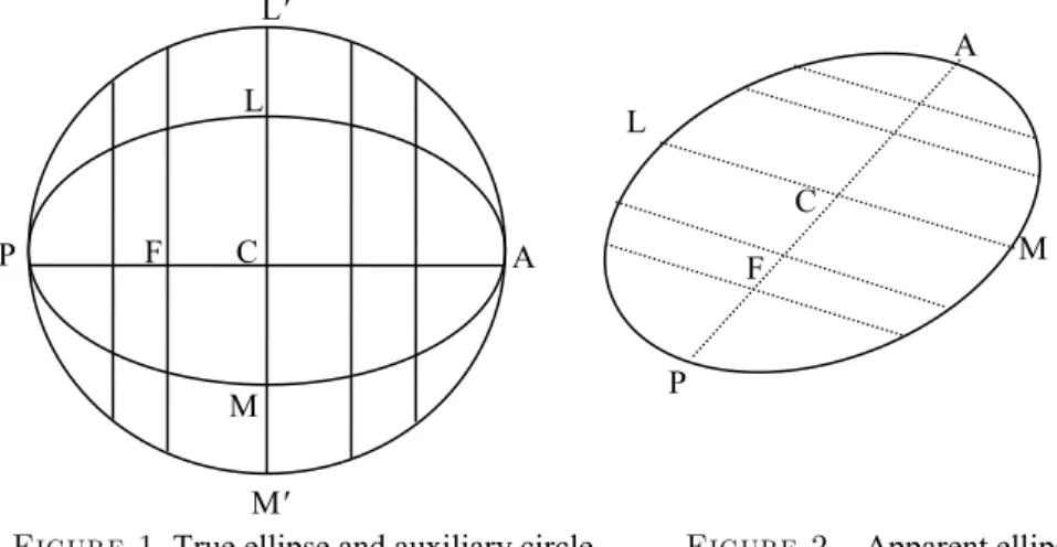
methods for computing the true orbit elements such as the Kowalsky's (Smart 1949), Zwier's (Smart 1949), or Atkinson methods (Atkinson 1966). Using these methods requires extensive amount of computations. In contrast, I present an analytical method for constructing the auxiliary ellipse, which allows for closed form formulas for computing the orbit elements as shown later. Astronomers have used the auxiliary circle depicted as AL'PM' in Fig. 1 to retrieve the true data. Before probing into that, some aspects of projection geometry are introduced. Angles between lines may not be preserved but parallel lines remain so in projection;

a line may shrink but its segments will maintain their proportions. Another preserved property is the ellipse conjugate diameters. An ellipse diameter is any chord that passes through its center; a diameter is conjugate to another diameter if it bisects it and all the chords that are parallel to it. The motive for using the auxiliary circle is that one of its diameters (the one that is parallel to the plane of view) will not be shrunken by the projection. This diameter, once obtained, allows for determining all the orbital elements. Examining Fig. 1, helps the understanding of the construction process of the auxiliary ellipse (Hilditch 2001). The figure shows that both the true orbit ellipse ALPM and the auxiliary circle AL'PM' share the diameter PFCA that is conjugate to LCM. If e is the true ellipse eccentricity, then from analytical geometry the ordinates of the ellipse are scaled down ordinates of the circle by a factor K, given by

2

1

K  e (2)

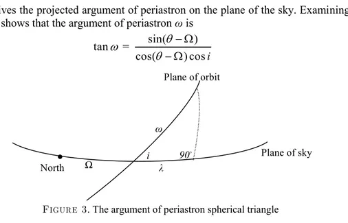
For example CL =CL' K. As mentioned, this property is preserved in projection. Figure 2 depicts the apparent ellipse which is the projection of the true ellipse. It shows the PFCA diameter and its conjugate LCM. The auxiliary ellipse (projection of auxiliary circle) can be constructed by scaling up the lengths of the conjugate

P A L' M' C L M F C P A M L F

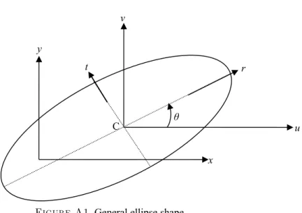
diameter LCM and its parallels by 1/K. The equations of these lines are given in the literature and provided also for completeness in Eq. (7) below. First, one needs to compute the intersections of these lines with the ellipse for at least five points. Next, compute the coordinates that scale up the chord lengths by 1/K. These new coordinates will now be points on the auxiliary ellipse which are used to compute the ellipse coefficients. Figure 4 depicts an example of an apparent ellipse and its constructed auxiliary one. Instead of this numerical process, our approach is to solve for the auxiliary ellipse coefficients analytically.

Eccentricity Computation

Herein, we adopt the notation that F is the origin of the apparent ellipse and ,x y is

its center. If the equation of the major axis of the apparent ellipse isymxand its slope ism y x/ , then it intersects its border at

2 2 2 2 2 2 2 2 2 2 2 2 2 2 2 0 ( 2 ) 2( ) 0 ( 2 ) 2( ) 0 2 0 ax hmx bm x gx fmx c a hm bm x g fm x c ax hxy by x gx fy xx cx Lx Lxx cx L c L c x x x y y y L L                                 (3)

Therefore the apastron and periastron coordinates are respectively given by

A , P , L c L c x x y y L L L c L c x x y y L L  _{ }  _   _    _{ }  _   _   (4)

It is worth noting that while C is the center of both the apparent and the true ellipses, F is not the focus of the apparent ellipse, but the ratio of FC to PC is preserved. If

2 2

FC r  x y , then Eq. (4) shows thatAC PC r



L c



/L. Thus if the true ellipse eccentricity is e, then

FC r L e PC L c L c r L      (5)

which implies that 2 L ₁ 2 c e e L c L c       

Parametric Representation of the Apparent Ellipse

Since the projected major axis passes through the points F(0,0) and the center C

( , )x y , then any point on this line can be represented by (

 

x, y), where α is a parameter variable. Herein, we refer only to the latus rectum that passes through the primary star. If the equation of this latus rectum isy mx, (m=-g/f), then it intersects the ellipse at, see derivation of Eq.(3),

2 2 2 2 2 2 2 2 ( 2 ) 2( ) 0 ( 2 ) 0 0 /( ) /( ) a hm bm x g fm x c af hfg bg x cf Llx cf x f c Ll y g c Ll                   (6)

The equation of any line parallel to the latus rectum is

fy  gx d (7)

If this line passes through a point (

 

x, y)(which is a point on the major axis) then it must satisfy Eq.(7); this implies that

f y



 g x



  d d



gx



fy (8) Substituting for d in Eq. (7) gives,









fy gx gx fy f y y g x x y y g x x f













              (9)

If this line intersects the ellipse at (u,v), then parametrically Eq. (9) can be represented by v y gs u x fs        (10)

from which we can find that

( ) fv gu gx fy L fv gu L             (11)

2 2 2 2 2 2 2 0 ( ) 2 ( )( ) ( ) 2 ( ) 2 ( ) 0 au huv bv gu fv c a x fs h x fs y gs b y gs g x fs f y gs c                          (12) Expanding and collecting terms of the above equation results in

2 2 2 2 2 2 ( 2 ) 2 [( ) ( ) ] 2 ( ) ( 2 ) 0 ax hxy by af hg x bg hf y s gx fy af hfg bg s c







             (13)

Using Eqs. (A.3), (A.4) and (A.8) in Eq. (13) yields

2_{L 2 ( lyx lxy s) 2 L lLs}2 _c 2_{L 2 L lLs}2 _{c 0}

              

from which s can be solved, 2 2 2 c L/ s l

 

   (14)

Geometrically, the parameter s represents the distance between the two points

(

 

x, y) and (u,v). If this distance is lengthened by a factor 1/K, (where K as given by Eq. (2)) then the new length will be

s s

K

  (15)

The above two equations give

2 2 2 2 c L/ s K l

 

    (16)

The scaled up ellipse is now given by, see Eq. (10)

v y gs u x fs          (17)

From the above we note that,

gu fv

L

     (18)

Equation of the Auxiliary Ellipse

To get the equation of the scaled up ellipse the parameter α must be eliminated from Eq. (17) and simultaneously from s'. One approach is to rewrite Eq. (17) as follows















2 _{2 2} 2 2 2 2 u x f s u x v y fgs v y g s                (19)

Now multiply the first equation by a, the second by 2h, the last by b and add up to get,























2 2 _{2 2 2} 2 2 2 2 2 2 2 2 2 2 2 2 ( ) ( 2 ) 2 a u x h u x v y b v y s af hfg bg

au hu v bv axu hyu byv hxv ax hxy by

af hfg bg s                                   (20) The coefficient of α in Eq. (20), via Eqs.(A.2) and (18), can be simplified to

(axuhyubyvhxv)(axhy u) (by hx v )  (gu fv)



L Using the above equation and Eqs. (A.4), (A.8), (18) and (16) in Eq. (20) yields





2 2 2 2 2 2 2 2 2 2 2 2 2 2 2 2 2 2 2 2 2 2 / 2 2 2 2 / 0 2 (1 ) 2 0 c L au hu v bv L L lL lK aK u hK u v bK v LK L c L aK u hK u v bK v L K L c                                          (21)

Finally we substitute from Eq. (18) in the above





2 2 2 ₂ 2 2 2 ₍₁ 2₎ gu fv _{2 0} aK u hK u v bK v L K gu fv c L            _{ }        (22) Then Eq. (22) becomes

_{a u }2 _{2h u v  b v }2 _2



_{gu fv}



_{  c 0 (23)} where, 2 (1 K ) n L   and 2 2 2 2 2 a K a ng h K h nfg b K b nf          (24)

This is the equation for any scaled up ellipse. It becomes the equation of the auxiliary ellipse by specializing it to our case for which_K2 _{ 1 e}2_{andn e L}2 _.

Using Eq. (5) allows these two parameters to be expressed as:

2 2 2 1 1 1 c K e L c K n L L c          (25)

from which the auxiliary ellipse can be expressed by

2 2 ( ) ( ) ( ) a n ca g h n ch fg b n cb f             (26) The lengths of the semi-axes of the auxiliary ellipse A and B are now given by





















2 2 2 2 4 L c A a b D L c B a b D D b a h               (27)

The semi-major axis A is unaffected by the projection and represent the true radius of the auxiliary circle, but B is scaled down by cos i, where i is the inclination of the orbit plane to the plane of the sky, therefore

1 1 cos ( / ) cos a b D i B A a b D         (28)

Note that the argument of the arc cosine in Eq. (28) is nonnegative, thus its solutions fall in the first and fourth quadrants. By definition i should be in the range between 0° and 180°. Thus we select i to be between 0° and 90° for counter clockwise motion and between 90° and 180° for clockwise motion. Next we compute the position angle of the first node



relative to the North. Note that the line of nodes of the true orbit is parallel to the major axis of the auxiliary ellipse, thus



is the same as the slope of the major axis. From Eq. (A.5) the slope angle is given by

-1 1 2 tan 2 h b a   _   _     (29)

There is an ambiguity of 180° in Eq.(29); however, the first node is the one with

180

 

. In the absence of radial velocity data, it is not known whether this is the angle of the ascending or descending node. Resolving this ambiguity will result in determining



. It remains to determine the argument of the periastron ω. This angle is measured from the first node in the direction of motion of the secondary and runs from 0° to 360°. As with any celestial orbit, we see that its major axis passes by four points: periastron P, primary star at the focus F, center of the elliptical orbit C, and the apastron A. In the plane of the sky, the projection of the major axis still passes through these four points. However, we determine both the primary star and the center of the apparent ellipse. Joining these two points allows us to determine the projected major axis slope, θ.

1

tan y

x

 _ 

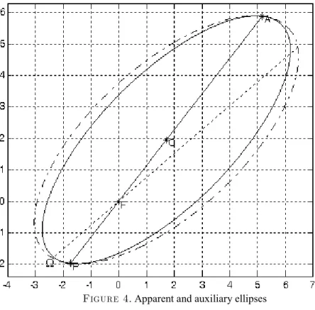
(30) Extending it both sides (until intersecting with the ellipse) will determine the positions of the periastron and apastron as given by Eq.(4). The angle difference between this line and the line of nodes, λ,

 

   (31)

gives the projected argument of periastron on the plane of the sky. Examining Fig. 3 shows that the argument of periastron ω is

sin( ) tan = cos( ) cos i        (32) Summary The steps to convert the apparent ellipse equation

2 ₂ 2 _{2 2 0}

ax  hxy by  gx fy c  (33)

to the auxiliary ellipse are summarized as follows, illustrated with a numerical example starting from a hypothetical apparent ellipse with equation (Tatum 2016)

λ 90◦ i ω Plane of sky Plane of orbit ● Ω North

2 2

14 -23x xy18 -3 -31 -100 0y x y 

1. compute the center point

2 2 =1.713987 1.956159 hf bg x ab h hg af y ab h        (34)

2. compute the coefficients of the auxiliary ellipse as follows





32.891445 1 0.00752494 L gx fy n L c        (35) 2 2 ' ( ) 10.55185 ( ) 8.478725 ( ) 15.35276 1.5 15.5 100. a n ca g h n ch fg b n cb f g g f f c c                               (36)

3. the equation of the auxiliary ellipse is now given by

2 2

st

True eccentricity = 0.497500

Lengths of semi axes , 5.665411 , 2.471021 Position angle of the 1 node 127° 05'

Inclination angle 64 08 ' 11 41' Argument of periastron 25 21' e nL A B i            

The apparent and auxiliary ellipses are depicted in Fig. 4. Appendix

Characteristics of Equation of Ellipse The following is a general equation of an ellipse

2 ₂ 2 _{2 2 0}

ax  hxy by  gx fy c  (A.1)

provided that





2 ₀

ab h a gx fy c 

where ,x y is its center point that satisfies the following

0 0 ax hy g hx by f       (A.2) hence 2 2 hf bg x ab h hg af y ab h       (A.3)

The variables L, l and D, used frequently, denote









2 2 2 2 ₂ 2 4 L ax hxy by gx fy l ab h D a b h            (A.4)

The tilt θ of the major axis of the ellipse with respect to the x-axis is

2 tan 2 h

b a

  

 (A.5)

One may note that there is an ambiguity of 90° in computing θ. To determine the ellipse semi major and semi minor axes we shift the origin of Eq. (A.1) to the center given by Eq. (A.3), then rotate the shifted axes by angle θ. The equation of the ellipse in the rotated frame becomes





















2 2 2 2 0 2 2 2 0 a b D a b D r t gx fy c a b D r a b D t L c                    (A.6) The major and minor axes are now given by

















2 2 L c 2 2 L c A B a b D a b D         (A.7)

Using Eq. (A.3) in the following we obtain

2 2 2 2 2 ( ) ( ) ( ) 2 j af hfg bg f af hg g bg hf fyl gxl l gx fy lL j af hfg bg lL                    (A.8)

Acknowledgement The author is profoundly grateful to Prof. Jeremy Tatum for thoroughly reviewing and editing the paper and for Prof. M. Hafez, N. Bekir and A. Bekir for editing the paper and suggesting many improvements.

References

[1] Atkinson, R. d'E. , "A New Method for Deriving the True Orbit of a Visual Binary", Astronomical Society of the Pacific, Vol. 78, No. 463, p.242, 1966. [2] Argyle, Bob (editor), Observing and Measuring Visual Double Stars, Springer

LLC 2004.

[3] Hilditch, R.W., An Introduction to Close Binary Stars, Cambridge, University Press 2001.

[4] Kallrath, J. and Milone, E., Eclipsing Binary Stars: Modeling and Analysis, Springer LLC 2009.

[5] Mullaney, James, Double and Multiple Stars and How to Observe Them, Springer 2005.

[6] Tatum, J.B., Celestial Mechanics, Chapter 17, "Visual Binary Stars",Updated 2016, "astrowww.phys.uvic.ca/~tatum/celmechs.html"

[7] Smart, W.M., Text-Book on Spherical Astronomy, Cambridge, University Press 1949.

Current Address: Esmat BEKIR: 5805 Serrania Avenue, Woodland Hills,

California, USA, 91367

E-mail: ebekir@hotmail.com

Orcid ID: https://orcid.org/0000-0001-8500-5131

v x y u θ C r t