Introduction to the fractional fourier transform and its applications

(1)

ADVANCES IN IMAGING AND ELECTRON PHYSICS. VOL . LO6

Introduction to the Fractional Fourier Transform and Its

Applications

Haldun M

.

Ozaktas and M

.

Alper Kutay Deparfnient of Electricul Engineering

Bilkent University TR-06533 Bilkent. Ankara. Turkey

David Mendlovic

Faculty qf Engineering. Tel-A viv University 69978 Tel.Aviv

.

Israel

1 . Introduction . . . 239

I I . Notation and Definitions . . . 243

I11 . Fundamental Properties . . . 245

IV . Common Transform Pairs . . . 247

V . Eigenvalues and Eigenfunctions . . . 249

V1 . Operational Properties . . . 252

VII . Relation to the Wigner Distribution . . . 256

VIII . Fractional Fourier Domains . . . 260

IX . Differential Equations . . . 261

X . Hyperdifferential Form . . . 263

XI. Digital Simulation of the Transform . . . 263

XI1 . Applications to Wave and Beam Propagation . . . 265

A . Introduction . . . 265

B . Quadratic-Phase Systems as Fractional Fourier Transforms . . . 268

C . Propagation in Quadratic Graded-Index Media . . . 270

D . Fresnel Diffraction . . . 271

E

.

Fourier Optical Systems . . . 273

F . Optical Implementation of the Fractional Fourier Transform 275 G . Gaussian Beam Propagation . . . 276

XI11 . Applications to Signal and Image Processing . . . 279

Acknowledgments . . . 286

References . . . 286

. . .

I

.

INTRODUCTION

The purpose of this chapter is to provide a self-complete introduction to the fractional Fourier transform for those who wish to obtain an understanding of the essentials without having to work through the hundreds of papers

(2)

240 HALDUN M. OZAKTAS, M. A. KUTAY, AND DAVID MENDLOVIC which have appeared in the last few years. A general introduction will be followed by the definition of the transform and a discussion of its fundamental and operational properties. Of central importance is the relationship of the transform to the Wigner distribution and other phase-space distributions (also known as time-frequency or space-frequency representations). We will concentrate on two main application areas which have so far received the most attention: wave and beam propagation and signal processing.

The fractional Fourier transform is a generalization of the ordinary Fourier transform with an order parameter a. Mathematically, the ath order fractional Fourier transform is the ath power of the Fourier transform operator. The a = 1st order fractional transform is the ordinary Fourier

transform. With the development of the fractional Fourier transform and related concepts, we see that the ordinary frequency domain is merely a special case of a continuum of fractional Fourier domains, and we arrive at a richer and more general theory of alternate signal representations, all of which are elegantly related to phase-space distributions. Every property and application of the common Fourier transform becomes a special case of that of the fractional transform. In every area in which Fourier transforms and frequency domain concepts are used, there exists the potential for generalization and improvement by using the fractional transform. For instance, the well-known result stating that the far-field diffraction pattern of an aperture is in the form of the Fourier transform of the aperture can be generalized to state that at closer distances, one observes the fractional Fourier transform of the aperture. The theory of optimal Wiener filtering in the ordinary Fourier domains can be generalized to optimal filtering in fractional domains, resulting in smaller mean-square errors at practically no additional cost.

In essence, the ath order fractional Fourier transform interpolates between a function f(u) and its Fourier transform &). The 0th order transform is simply the function itself, whereas the 1st order transform is its Fourier transform. The 0.5th transform is something in between, such that the same operation that takes us from the original function to its 0.5th transform will take us from its 0.5th transform to its ordinary Fourier transform. More generally, index additivity is satisfied: The a,th transform of the a,th transform is equal to the (az

+

u,)th transform. The - lth transform is the inverse Fourier transform, and the -ath transform is the inverse of the ath transform.

Scattered early papers related to the fractional Fourier transform include Wiener [1929], Condon [1937], Bargmann [1961], and de Bruijn [1973]. Of importance are two separate streams of mathematical papers which appeared throughout the eighties [Namias, 1980; McBride and Kerr, 1987;

(3)

FRACTIONAL FOURIER TRANSFORM AND ITS APPLICATIONS 241 Mustard, 1987a,b, 1989, 1991, 19961. However, the number of publications exploded only after the introduction of the transform to the optics and signal processing communities [Seger, 1993; Lohmann, 1993; Ozaktas and Mendlovic, 1993a,b; Mendlovic and Ozaktas, 1993; Ozaktas and others, 1994a; Alieva and others, 1994; Almeida, 19943. Not all of these authors were aware of each other or building on the work of those preceding them, nor is the transform always immediately recognizable in some of these works.

The fractional Fourier transform (or essentially equivalent transforms) appears in many contexts, although it has not always been recognized as being the fractional power of the Fourier transform and thus referred to as the fractional Fourier transform. For instance, the Green’s function of the quantum-mechanical harmonic oscillator is the kernel of the fractional Fourier transform. Also, the fractional Fourier transform is a special case of the more general linear canonical transform (see Wolf [1979] for an introduction and references). This transform has been studied in many contexts, but again the particular special case which is the fractional Fourier transform has usually not been recognized as such.

The preceding citations do not represent a complete list of known historical references. For a more complete list and also a more comprehen- sive treatment of the fractional Fourier transform and its relation to phase-space distributions, we refer the reader to a forthcoming book on the subject by the authors (Wiley, to be publ. 1999). We expect further scattered historical references not known to us to be revealed in time. Given the multitude of contexts in which essentially equivalent or closely related integral transforms appear, it is probably not possible to attribute its invention to a particular set of authors. These many contexts in which it was reinvented time after time in different guises is testimony to the elegance and ubiquity of the transform.

Given the widespread use of the ordinary Fourier transform in science and engineering, it is important to recognize this integral transform as the fractional power of the Fourier transform. Indeed, it has been this recognition which has inspired most of the many recent applications. Replacing the ordinary Fourier transform with the fractional Fourier transform (which is more general and includes the ordinary Fourier transforms as its special case) adds an additional degree of freedom to the problem, represented by the order parameter a. This in turn may allow either a more general formulation of the problem (as in the diffraction from an aperture example) or improvements based on the possibility of optimizing over a (as in the optimal Wiener filtering example).

The fractional Fourier transforms has been found to have several appli- cations in the area known as analog optical information processing, or

(4)

242 HALDUN M. OZAKTAS, M. A. KUTAY, A N D DAVID MENDLOVIC

Fourier optics. This transform allows a reformulation of this area in a way much more general than that found in standard texts on the subject. It has also led to generalizations of the notions of space (or time) and frequency domains, which are central concepts in signal processing, leading to many applications in this area. More generally, the transform may be expected to have an impact in the form of deeper understanding or new applications in every area in which the Fourier transform plays a significant role, and to take its place among the standard mathematical tools of physics and engineering.

More specifically, some applications which have already been investigated or suggested include diffraction theory [Alieva and others, 1994; Gori, Santarsiero, and Bagini, 1994; Pellat-Finet, 1994; Pellat-Finet, 1995; Ozak- tas and Mendlovic, 1995; Abe and Sheridan, 1995a; Alonso and Forbes, 1997; Ozaktas and Erden, 19971, optical beam propagation and spherical mirror resonators (lasers) [Ozaktas and Mendlovic, 1994; Erden and Ozaktas, 1997; Ozaktas and Erden, 19971, propagation in graded index media [Ozaktas and Mendlovic, 1993a,b; Mendlovic and Ozaktas, 1993; Mendlovic, Ozaktas, and Lohmann, 1994a; Alieva and Agullo-Lopez, 1995; Abe and Sheridan, 1995b; Gomez-Reino, Bao, and Perez, 19961, Fourier optics [Bernardo and Soares, 1994a,b; Pellat-Finet and Bonnet, 1994; Ozaktas and Mendlovic, 1995; Ozaktas and Mendlovic, 19961, statistical optics [Erden, Ozaktas, and Mendlovic, 1996a, b], optical systems design [Dorsch, 1995; Dorsch and Lohmann, 1995; Lohmann, 19951, quantum optics [Yurke and others, 1990; Aytur and Ozaktas, 19951, radar and phase retrieval [Raymer, Beck, and McAlister, 1994a,b; McAlister and others, 19951, tomography [Beck and others, 1993; Smithey and others, 1993; Lohmann and Soffer, 1994; Wood and Barry, 1994a,b], signal detection, correlation, and pattern recognition [Mendlovic, Ozaktas, and Lohmann, 1995d; Alieva and Agullo-Lopez, 1995; Garcia and others, 1996; Lohmann, Zalevsky, and Mendlovic, 1996b; Bitran and others, 1996; Mendlovic and others, 1995a; Mendlovic, Zalevsky, and Ozaktas, 19981, space- or time- variant filtering [Ozaktas and others, 1994a; Granieri, Trabocchi, and Sicre, 1995; Mendlovic and others, 1996b; Ozaktas, 1996; Zalevsky and Men- dlovic, 1996; Mendlovic and others, 1996b; Kutay and others, 1997; Mus- tard, 19971, signal recovery, restoration, and enhancement [Lohmann and others, 1996a; Erden and others, 1997a,b; Ozaktas, Erden, and Kutay, 1997; Kutay and Ozaktas, 1998; Kutay and others, 1998a,b], multiplexing and data compression [Ozaktas and others, 1994a1, study of space- or time- frequency distributions [Almeida, 1994; Fonollosa and Nikias, 1994; Loh- mann and Soffer, 1994; Ozaktas and others, 1994a; Mendlovic and others, 1995c; Dragoman, 1996; Mendlovic and others, 1996a; Ozaktas, Erkaya, and Kutay, 1996a; Mihovilovic and Bracewell, 19913, and solution of

(5)

FRACTIONAL FOURIER TRANSFORM AND ITS APPLICATIONS 243 differential equations [Namias, 1980; McBride and Kerr, 19871. We believe that these are only a fraction of the possible applications. We hope that this chapter will make possible the discovery of new applications by introducing the subject to new audiences.

11. NOTATION AND DEFINITIONS

The ath order fractional Fourier transform of the function f ( u ) will most often be denoted by f a ( u ) or, equivalently, Faf(u). When there is possibility of confusion, we may more explicitly write @'[f(u)]. The transform is defined as a linear integral transform with kernel K,(u, u'):

f,(~)

= F [ , f ( u ) ] =

J

K,(u, u ' ) f ( u ' ) du'.

The kernel will be given explicitly in the following text. All integrals are from minus to plus infinity unless otherwise stated. We prefer to use the same dummy variable u both for the original function in the space (or time) domain and its fractional Fourier transform. This is in contrast to the conventional practice associated with the ordinary Fourier transform, where a different symbol, say p, denotes the argument of the Fourier transform

w:

F ( p ) = s f ( u ) e - i 2 f f p u du, (2)

f ( u ) =

s

F(p)ei2"fiU d p . (3)

s

But these can be rewritten as

F(u) = f ( ~ ' ) e - " ~ " ~ ' du' (4)

dp'. ( 5 )

f ( u ) =

1

F(u' )ei2xu'u

When it is desirable to distinguish the argument of the transformed function from that of the original function, we will let u, denote the argument of the ath order fractional Fourier transform: f,(u,) = (Fa [f(u)])(u,). With this convention, u,, corresponds to u, the space (or time) coordinate; u1 corre- sponds to the spatial (or temporal) frequency coordinate p ; and u2 = -uo,

u3 = -ul. Finally, we will agree to always interpret u as a dimensionless variable.

(6)

244 HALDUN M. OZAKTAS, M. A. KUTAY, A N D DAVID MENDLOVTC We will refer to 9;“[.], or simply

Pa,

as the ath order fractional Fourier transform operator. This operator transforms a function f ( u ) into its fractional Fourier transform f,(u). We will restrict ourselves to the case where the order parameter a is a real number. The signal ,f is a finite energy signal and f ( u ) is a finite energy function both of which are well behaved in the sense usually presumed in physical applications. In quantum mechanics

f is the abstract state vector

I f )

and f ( u ) = ( u l f ) is the u-representation of J: Likewise, f,(u) = (u,If) is the u,-representation, which we will also refer to as the representation of f in the ath order fractional Fourier domain. In this context If(u)l’ is interpreted as a probability distribution so that the energy of the function En[f] = flf(u)l’du =

(,fl.f)

corresponds to

its integrated probability and is thus equal to 1. In signal processing and optics, the energy can take on any finite value but is conserved if attenuation or amplification mechanisms do not exist. (We will also deal with sets of signals and functions whose energies are not finite (delta functions and harmonic functions); these will not correspond to physically realizable functions, but rather serve as intermediaries in our formulations.)

We now define the ath order fractional Fourier transform f,(u) through the following linear integral transform:

f,(u) =

s

K,(u, u ’ ) f ( u ’ ) du‘, (6) K,(u, u’) = A , exp[ir(cot u2

-

2 csc

4

uu‘

+

cot

4

u ‘ ~ ) ] .

where

A, = JI - icotd. ₍₈₎

The square root is defined such that the argument of the result lies in the interval (-n/2,

421.

The kernel is not strictly defined when a is an even integer. However, it is possible to show that as a approaches an even integer, the kernel behaves like a delta function under the integral sign. Thus, consistent with the limiting behavior of the above kernel for values of a approaching even integers (further discussed later), we define Klj(u, u‘)

= 6(u - u’) and K A j k 2 ( u , u’) = 6(u

+

u’), where j is an arbitrary integer. Generally speaking, the fractional Fourier transform of f ( u ) exists under the same conditions under which its Fourier transform exists [McBride and Kerr, 1987; Almeida, 19943.

(7)

FRACTIONAL FOURIER TRANSFORM AND ITS APPLICATIONS 245

111. FUNDAMENTAL PROPERTIES

We first examine the case when a is equal to an integer j . We note that by definition P4’ and F4j+2 correspond to the identity operator

9

and the parity operator

9,

respectively (that is, f4j(u) = f ( u ) and f4j+2(u) =

f(

- u)). For a = 1 we find

4

= 4 2 , A , = 1, and

fi(u) = exp(- i2nu211),f(u’) du’. (9)

We see that f,(u) is equal to the ordinary Fourier transform of f(u), which

was previously denoted by the conventional upper case F(u). Likewise, it is possible to see that F - ,(u) is the ordinary inverse Fourier transform of f’(u).

Our definition of the fractional Fourier transform is consistent with defining integer powers of the Fourier transform through repeated application (that is, P 2 = 9797, F 3 = 97F2, and so on). Since

I$

= an12 appears in Equation

6 only in the argument of trigonometric functions, the definition is periodic in u (or

4)

with period 4 (or 2.n). Thus it is sufficient to limit attention to

the interval a E [ - 2,2). These facts can be restated in operator notation:

9-0 = 6, 9-1 = <F, F 2 = 9, 9 3 = 99 = Y<F, 974 = F O = 3 > 9 4 j t a - - 9 4 j ’ + a where j , j ‘ are arbitrary integers.

Let us now examine the behavior of the kernel for small la1 > 0:

- insgn(d4)/4

exp[i.n(u

- u’)~/I$].

Ja

K,(u,u‘) =

Now, using the well-known limit

the kernel is seen to approach 6(u - u’) as u approaches 0. Thus defining the kernel Ka(u, u ’ ) to be precisely S(u - u’) at a = 0 maintains continuity of the transform with respect to a. A similar discussion is possible when a

(8)

246 HALDUN M. OZAKTAS, M. A. KUTAY, A N D DAVID MENDLOVIC approaches other integer multiples of 2. A more rigorous discussion of continuity with respect to a may be found in McBride and Kerr [1987].

We now discuss the index additivity property:

p ' p y ( U ) = p a 1 +"'f(U) = g-:"'p-"'f(u),

or in operator notation

g a l o j r a z = y a l + a 2 = _{4 4 .}o-azo-a!

This can be proved by repeated application of Equation 6, showing

Ku2(u, u")K,,(u", u') du" = K,, + a 2 ( ~ , u')

s

(19) and amounts to

by direct integration, which can be accomplished by using standard Gaus- sian integrals. We do not present the details of this proof, since this property will follow much more simply from certain properties of the transform to be discussed.

The index additivity property is of central importance. Indeed, without it, we could hardly think of Fa as being the ath power of 9 (more will be said on this later). For instance, the 0.2nd fractional Fourier transform of the 0.5th transform is the 0.7th Fourier transform. Repeated application leads to statements such as, for instance, the 1.3th transform of the 2.lst transform of the 1.4th transform is the 43th transform (which is the same as the 03th transform). Transforms of different orders commute with each other so that their order can be freely interchanged. From the index additivity property, we deduce that the inverse of the ath order fractional Fourier transform operator (Fa)-' is simply equal to the operator

F-,

(because 9-"Fa = 3). This can also be shown by directly demonstrating that

K,(u, u")K -,(u", u') du = 6 ( ~ - u'), ₍₂₁₎ so that K ; '(u, u') = K-,(u, u'). Thus we see that we can freely manipulate the order parameter a as if it denoted a power of the Fourier transform operator

F.

Fractional Fourier transforms constitute a one-parameter family of transforms. This family is a subfamily of the more general family of linear canonical transforms which have three parameters [Wolf, 1979; Mohinsky and Quesne, 1971; and Mohinsky, Seligman, and Wolf, 19721. As all linear canonical transforms do, fractional Fourier transforms satisfy the associa- tivity property and they are unitary, as we can directly see by examining the

(9)

FRACTIONAL F O U R I E R T R A N S F O R M AND ITS A P P L I C A T I O N S 247

kernel of the inverse transform obtained by replacing a with --a:

KO- ‘(u, u‘) = K - , ( u , u‘) = K,*(u, u’) = K,*(u’, u). ₍₂₂₎ The kernel K,(u, u’) is symmetric and unitary, but not Hermitian. Unitarity implies that the fractional Fourier transform can be interpreted as a transformation from one representation to another, and that inner products and norms are not changed under the transformation.

IV. COMMON TRANSFORM PAIRS

Table 1 gives the fractional Fourier transforms of a number of functions for which the integral appearing in Equation 6 can be evaluated analytically (often using standard Gaussian integrals). More will be said on the fractional Fourier transforms of chirp functions exp[in(Xu2

+

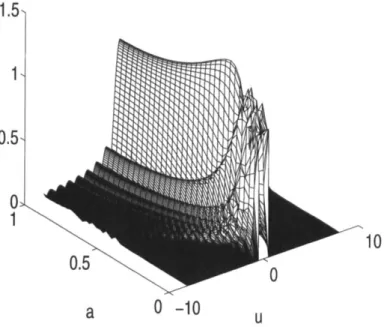
25u)] after we discuss the Wigner rotation property of the transform.

Greater insight can be obtained by considering some numerically obtained illustrations. Indeed, the fractional Fourier transforms of many common functions do not have simple closed-form expressions. These may be obtained numerically using the algorithm discussed in Section 11 later. We know that when a = 0 we have the original function, and when a = 1

we have its ordinary Fourier transform. As a varies from 0 to 1, the transform evolves smoothly from the original function to the ordinary Fourier transform. Figures 1 and 2 show the evolution of the rect(u)

TABLE 1

THE FUNCTIONS ON THE RIGHT ARE THE FRACTIONAL FOURIER TRANSFORMS OF THE FUNCTIONS ON THE LEFT; j IS AN ARBITRARY INTEGER, AND ( AND

x

ARE REAL CONSTANTS. FOR CERTAIN

(EQUATION 17). IN THE LAST PAIR, x z 0 IS REQUIRED FOR CONVERGENCE. ISOLATED VALUES OF (1, THE EXPRESSIONS BELOW SHOULD RE INTERPRETED IN THE LIMITING SENSE

(10)

248 HALDUN M. OZAKTAS, M. A. KUTAY, AND DAVID MENDLOVIC

a = O a=113

(c) (4

FIGURE 1. Magnitudes of the fractional Fourier transforms of the rectangle function, I.

function into the sinc(u) E (sinw)/(nu) function. Figure 3 shows the real parts of the fractional Fourier transforms of the Dirac delta function

6(u - 1). We note that for orders close to zero, the transform of the delta function is highly oscillatory, and thus will approximately behave like the delta function under the integral sign, averaging out to zero whatever function it happens to multiply.

Finally, we give the fractional Fourier transform of the quadratic phase function f(u) = exp( - 4 4 )

f i

exp(inu2/r,) with complex radius rc:

provided Y(r,) d 0, which is also the condition for the original function f(u) to have finite energy. From this result we conclude that the complex radius

(11)

FRACTIONAL FOURIER TRANSFORM AND ITS APPLICATIONS ₂₄₉

FIGURE 2. Magnitudes of the fractional Fourier transforms of the rectangle function, 11.

r: of the transformed function is

rc

+

t a n 4 ' 1 - r,tan$ r', =

This result is useful in beam propagation problems since the original function f(u) represents a Gaussian beam with complex radius rc.

V. EIGENVALUES AND EIGENFUNCTIONS

The eigenvalues and eigenfunctions of the ordinary Fourier transform are well known (although seldom discussed in introductory texts). They are the Hermite-Gaussian functions t+hn(u), commonly known as the eigensolutions of the harmonic oscillator in quantum mechanics, or the modes of propagation of quadratic graded-index media in optics. The eigenvalues may be expressed as exp( - in742) and are given by 1, - i, - 1, i, 1,

-

i,

. . .

for n = 0, 1, 2, 3, 4, 5,.

.

Thus the eigenvalue equation for the ordinary Fourier transform may be written as

(12)

250 HALDUN M. OZAKTAS, M. A. KUTAY, A N D DAVID MENDLOVIC 1.5- 1 . 0.5. 0 r 1 1.5 1 0.5 0 -0.5 -1 -1.5

where the Hermite-Gaussian functions are more explicitly given by

$"@) = A,H,(JGu)e-""', (26) for n = 0, 1, 2, 3, 4, 5 , .

. . .

Here H,(u) are the Hermite polynomials. The particular scale factors which appear in this equation are a direct consequence of the way we have defined the Fourier transform with 2n in the exponent.

The ath order fractional Fourier transform shares the same eigenfunctions as the Fourier transform, but its eigenvalues are the ath power of the eigenvalues of the ordinary Fourier transform:

(13)

FRACTIONAL FOURIER TRANSFORM AND ITS APPLICATIONS 25 1 This result can be established directly from Equation 6 by induction. First, we can show that ICl0(u) and $,(u) are eigenfunctions with eigenvalues 1 and exp(

-

ian/2) by evaluating the resulting standard complex exponential integrals. Then, by using standard recurrence relations for the Hermite- Gaussian functions it is possible to assume that the result-to-be-shown holds for n - 1 and n, and show that as a consequence it holds for n

+

1. This

completes the induction.

The preceding demonstrated outline of the fact that Hermite-Gaussian functions are eigenfunctions of the fractional Fourier transform as defined by Equation 6 then reduces to the well-known fact that Hermite-Gaussian functions are eigenfunctions of the ordinary Fourier transform when a = 1, since Equation 6 reduces to the definition of the ordinary Fourier transform and since e-ianx'Z reduces to

Readers familiar with functions F N ( d ) of an operator (or matrix) d with eigenvalues

A,,

will know that in general &"(d) will have the same eigenfunctions as d and that its eigenvalues will be F N ( I n ) . The above eigenvalue equation is particularly satisfying in this light since 9*, as we have defined it, is indeed seen to correspond to the ath power of the Fourier transform operator ( F N ( * ) = (.)"). However, it should be noted that the definition of the ath power function is ambiguous, and our definition of the fractional Fourier transform through Equation 6 is associated with a particular way of resolving the ambiguity associated with the ath power function (Equation 28). Other definitions of the transform also deserving to be called the fractional power of the Fourier transform are possible. The particular definition we are considering is the one that has been most studied and that has led to the greatest number of interesting applications. We are convinced it has a special place among other possible definitions.

Knowledge of the complete set of eigenvalues and eigenfunctions of a linear operator is sufficient to completely characterize the operator. In fact, in some works the fractional Fourier transform has been defined through its eigenvalue equation [Namias, 1980 Ozaktas and Mendlovic, 1993a, b; Mendlovic and Ozaktas, 19931. To find the fractional transform of a given function f(u) from knowledge of the eigenfunctions and eigenvalues only, we first expand the function as a linear superposition of the eigenfunctions of the fractional Fourier transform (which are known to constitute a complete set):

(14)

252 HALDUN M. OZAKTAS, M. A. KUTAY, A N D DAVID MENDLOVIC Applying 9" on both sides of Equation 29 and using Equation 28,

obtains

one

(31)

n = O J n = O

Upon comparison with Equation 6, the kernel K,(u, u') is identified as

m

K,(u, u') =

1

e-'an"/2 $n(U)$ n(u'). ₍₃₂₎ This is the spectral decomposition of the kernel of the fractional Fourier transform. The kernel given in Equation 32 can be shown to be identical to that given in Equation 6 directly by using an identity known as Mehler's formula:

n = O

Several properties of the fractional Fourier transform immediately follow from Equation 28. In particular the special cases a = 0, a = 1, and the index additivity property are deduced easily. (The latter can be shown by applying F'' to both sides of Equation 28.)

VI. OPERATIONAL PROPERTIES

Various operational properties of the transform are listed in Table 2

[Namias, 1980; McBride and Kerr, 1987; Mendlovic and Ozaktas, 1993;

Almeida, 19941. Most of these are most readily derived or verified by using Equation 6 or the symmetry properties of the kernel.

Operations satisfying the first property are referred to as even operations, so that the fractional Fourier transform is an even operation. This property also implies

which in turn imply that the transform of an even function is always even and the transform of an odd function is always odd. Similar facts can be stated in operator form: All even operators, and in particular the frac-

(15)

FRACTIONAL FOURIER TRANSFORM AND ITS APPLICATIONS 253 TABLE 2

OPERATIONAL PROPERTIES OF THE FRACTIONAL FOURIER TRANSFORM. 4 IS AN ARBITRARY REAL NUMBER, k Is A REAL NUMBER (k # 0, cu), AND n Is AN INTEGER; 4' = arctan(kz tand),

WHERE

4'

Is TAKEN T o BE IN THE SAME QUADRANT AS

4.

f ( u )

m)

tional Fourier transform operator, commute with the parity operator 9' ( F a y = 9'Fa) and satisfy F n = 9'.FaP. The eigenfunctions of even operations can always be chosen to be of definite (even or odd) parity (the Hermite-Gaussian functions satisfy this property).

The second property is the generalization of the ordinary Fourier trans- form property stating that the Fourier transform of f ( k u ) is

lkl-iF(p/k).

Notice that the fractional Fourier transform of f ( k u ) cannot be expressed as a scaled version of fa(u) for the same order a. Rather, the fractional Fourier transform of f ( k u ) turns out to be a scaled and chirp-modulated version of f,.(u) where a' # a is a different order.

Now we turn our attention to the fifth and sixth properties. The fractional Fourier transform of uf(u) is equal to a linear combination of ufa(u) and df,(u)/du. The coefficients of this linear combination are cos

4

and -sin

4.

When u = 1, this reduces to the corresponding ordinary Fourier transform

property. Similar comments apply to the fractional Fourier transform of df(u)/du. The essence of these properties are most easily grasped if we express them in pure operator form. Let us define the coordinate multiplication operator 4?l and differentiation operator 99 through their effects in the space domain

(16)

254 HALDUN M. OZAKTAS, M. A. KUTAY, A N D DAVID MENDLOVIC

operators of quantum mechanics and might have been written as

1 d i2n du

( u l W > =

-

(ulf). (39)

We may define in the same spirit operators %, and g,, which have the same effect on f,(u), the ath order fractional Fourier transform of f ( u ) :

where we have explicitly written u, to avoid confusion. The effect of these operators is to coordinate multiply and differentiate the fractional Fourier transform of f ( u ) , rather than f ( u ) itself. Now, with these definitions, the fifth and sixth properties of Table 2 can be written as

9'c"~f(41

= cos4(% f),(u,)

-

sin

$(9,f)&,),

S0[19f(41

= sin

$(%.f),(%)

+

cos d J @ , . f ) o ( ~ , ) .

(42) (43) (%,f),(u,) is simply the u, representation of

%,f,

which we also refer to as the representation of @, f in the uth fractional Fourier domain. In the notation of quantum mechanics, (42, f),(u,) would have been written as (u,l%,',f). Similar comments apply to (B,f),(u,). The two preceding equations can be written in abstract operator form as

We see that the coordinate multiplication and differentiation operators corresponding to order u are related to those in the ordinary space (or time) domain by a simple rotation matrix.

The commutator [%,

9 1

3

a9

- 9% is well known to be equal to i/2n.

By using Equation 44 we can easily derive the commutator [Aytur and Ozaktas, 1995; Ozaktas and Aytur, 19951:

Knowing the commutator of two operators allows one to deduce an uncertainty relation between the two representations associated with those

(17)

FRACTIONAL FOURIER TRANSFORM AND ITS APPLICATIONS 255 operators. In particular, the above commutation relation leads to [Aytur and Ozaktas, 1995; Ozaktas and Aytur,

19951

Here a*o is the standard deviation of

J f , ( ~ , ) 1 ~

and a.yl,. is the standard deviation of

Ifa,(~,.)1~.

The translation and phase shift operators can also be expressed in operator notation. Let

F ( 5 )

denote the operator which takes f ( u ) to f ( u -

5)

and let 9(5) denote the operator which takes f ( u ) to exp(i2n(u)f(u), all in the ordinary space domain. We may also define Fa(()

and

Po([)

as the operators which have the same effect on the ath order fractional Fourier transforms:

FJt)

takes f,(u,) to f,(u, -

5)

and Pa(<)

takes f,(u,) to exp(i27t5ua)f,(u,). Then the third and fourth properties of Table 2 can be expressed as [Aytur and Ozaktas, 1995; Ozaktas and Aytur,

1995)

q~[y(5)f(~)]

= eiz<2sin6cos4 _[2,(u _-

₅

_sin

_4)%(5

_cos

+)md

CYa(5 cos

4)9(5

sin

4)fI,(%)

-

e-i@sinq5cos6 9

(51)

-

eix<2sindcosq5 o-

-

_J,(5

_sin

_4PJ5

_cos

_4).

We again see that the effect of translation is a combination of translation (by C O S ~ ) and phase multiplication (by sinq5) of the fractional Fourier transform. A similar comment applies to the effect of phase multiplication. When a = 1, these results reduce to the corresponding well-known proper-

ties of the ordinary Fourier transform.

The fractional Fourier transform does not have a convolution or multiplication property of comparable simplicity to that of the ordinary Fourier transform.

(18)

256 HALDUN M. OZAKTAS, M. A. KUTAY, AND DAVID MENDLOVIC

VII. RELATION TO THE WIGNER DISTRIBUTION

The direct and simple relationship of the fractional Fourier transform to the Wigner distribution as well as to certain other phase-space distributions is perhaps its most important and elegant property [Mustard, 1989, 1996; Lohmann, 1993; Almeida, 1994; Mendlovic, Ozaktas, and Lohmann, 1994a; Ozaktas and others, 1994a1.

Here we will define and briefly discuss some of the most important properties of the Wigner distribution. The Wigner distribution W,(u, p) of a function f(u) is defined as

W,(u, p ) =

s

,f(u

+

u'/2)f*(u - u'/2)e-2"p"'du'. (52)

Wf

(u, p) can also be expressed in terms of F(p), or indeed as a function of any fractional transform of f(u). Some of its most important properties are

(55) Roughly speaking, W(u, p ) can be interpreted as a function that indicates the distribution of the signal energy over space and frequency. The Wigner distribution of F(u) (the Fourier transform of f(u)) is a ninety-degree rotated version of the Wigner distribution of f(u). More on the Wigner distribution and other such distributions and representations may be found in Claasen and Mecklenbrauker [1980a,b,c, 19931, Hlawatsch and Bou- dreaux-Bartels [1992], and Cohen [1989, 19951.

Now, if W,(u, p) denotes the Wigner distribution of f(u), then the Wigner distribution of the ath fractional Fourier transform of f(u), denoted by

WJa(u,

p ) , is given by

Wfn(u,

p ) = W,(u cos (6 - p sin (6, u sin (6

+

p cos (6). ₍₅₆₎ so that the Wigner distribution of Wm(u, p) is obtained from W,(u, p ) by rotating it clockwise by an angle

4.

Let us define 9?+ to be the operator which rotates a function of ( u , p ) by angle

4

in the conventional counter- clockwise direction. Then we can write

(57)

Wf,(U,

p) =

a-&w,(U,

p).

(19)

FRACTIONAL FOURIER TRANSFORM AND ITS APPLICATIONS 257 This elegant and fundamental property underlies an important number of the applications of the fractional Fourier transform. In fact, some authors have defined the transform as that operation which corresponds to rotation of the Wigner distribution of a function [Lohmann, 19931.

Equation 56 can be derived directly from Equation 6 and the definition of the Wigner distribution given by Equation 52 [Ozaktas and others, 1994a1. The derivation is somewhat lengthy but straightforward. A similar

derivation is given by Mustard [1989, 19961 and by Almeida [1994]. Lohmann [ 19931 shows the reverse, starting from the rotation property and arriving at Equation 6.

An at least equally important form of this result follows easily [Mustard, 1989, 1996; Lohmann and Soffer, 1994; Ozaktas and others, 1994a1. Let us recall Equations 53 and 54, which state that the integral projection of W,(u, p ) onto the u axis is the magnitude square of the u-domain represen- tation of the signal and that the integral projection of W,(u, p ) onto the p axis is the magnitude square of the p-domain representation of the signal. Now, let us rewrite the first of these equations for .f;(u), the uth order fractional Fourier transform of f ( u ) :

Since Wfa(u, p ) is simply W,(u, p ) clockwise rotated by angle

4,

the integral projection of Wfa(u, p ) onto the u axis is identical to the integral projection of W,-(u, p ) onto an axis making angle

4

with the u axis. This new axis making angle

4

= 4 2 with the u axis is referred to as the u, axis. Let .@.d9,1j denote the Rudon trunSform operator, which maps a two-dimen- sional function of (u, p ) to its integral projection onto an axis making angle

4

with the u axis [Bracewell, 19951. Thus the above can be written as

(59)

In conclusion, the integral projection of the Wigner distribution of a function onto the u, axis is equal to the magnitude square of the uth order fractional Fourier transform of the function (Fig. 4). Equations 53 and 54

are special cases with u = 0 and a = 1. Wood and Barry discussed what they

referred to as the “Radon-Wigner transform” without realizing its relation to the fractional Fourier transform [Wood and Barry, 1994a,b]. The above discussion demonstrates that the Radon-Wigner transform is simply the magnitude squared of the fractional Fourier transform.

The results of this section, and in particular Equation 59, continue to hold when W’(u, p ) is the Wigner distribution of a random process since the expectation value operation can move inside the Radon transform and

(20)

258 HALDUN M. OZAKTAS, M. A. KUTAY, AND DAVID MENDLOVIC

u,

FIGURE 4. Oblique integral projections of the Wigner distribution.

rotation operators:

W,,(U> PI = B-4, W,(% P I ,

a.dg+w,(K P ) =

l.Lt4IZ.

(61)

( 60)

_ _ _ _ _ _

Here the overbars denote ensemble averages.

The Wigner distribution is not the only time-frequency representation satisfying the rotation property (Equation 57). The ambiguity function also satisfies this property because the ambiguity function is the two-dimensional Fourier transform of the Wigner distribution, and the two-dimensional Fourier transform of the rotated version of a function is the rotated version of the two-dimensional Fourier transform of the original function [Ozaktas and others, 1994a; Almeida, 19941. Almeida [1994] showed that the rotation property also holds for the spectrogram. It has been further shown that the rotation property generalizes to certain other time-frequency distributions belonging to the so-called Cohen class, whose members can be obtained from the Wigner distribution by convolving it with a kernel characterizing that distribution. The distributions for which the rotation property holds are those which have a rotationally symmetric kernel [Ozaktas, Erkaya, and Kutay, 1996a1.

Thus, fractional Fourier transformation corresponds to rotation of many phase-space representations. This not only confirms the important role this

(21)

FRACTIONAL FOURIER TRANSFORM AND ITS APPLICATIONS 259 transform plays in the study of such representations but also supports the notion of referring to the axis making angle

4

= a 4 2 with the u axis as the ath ,fractional Fourier domain. Despite this generalization, the only distribu- tion which satisfies a relation of the form of Equation 59 is the Wigner distribution [Mustard, 19891. Cohen [I9891 argues that there is nothing special about the Wigner distribution among other members of the Cohen class, since all members of this class, including the Wigner distribution, are derivable from each other through convolution relations. However, the fact that only the Wigner distribution satisfies Equation 59 has led Mustard to suggest that the Wigner distribution is a specially distinguished member of the Cohen class [Mustard, 1989, 19961.

As an instructive application of the Wigner rotation property, we discuss

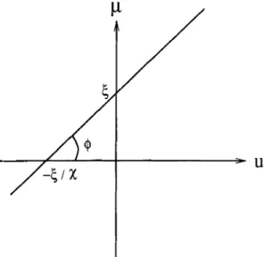
the fractional Fourier transforms of chirp functions. The transform of the chirp function exp[in(Xu2

+

2&)] was given in Table 1 as a rather complicated expression. Phase-space offers a much more transparent picture. The Wigner distribution of the chirp function exp[in(Xu2

+

25u)] is W’(u, p) =

S(,u - xu -

0,

which is simply a line delta in phase space along the line ,u =

xu

+

5

making angle orctan

(x)

with the u axis (Fig. 5). The Wigner distribution of exp(i2ntu) is W,(u, p) = 6 ( p -

5 )

and is seen to be a special

case in which the line delta is horizontal. Similarly, the Wigner distribution of 6(u -

5 )

is W’(u, p) = 6(u -

5 )

and is also seen to be a special case in

(22)

260 HALDUN M. OZAKTAS, M. A. KUTAY, AND DAVID MENDLOVIC which the line delta is vertical. (That the chirp indeed behaves like a delta function as

x,

5

cn can be shown by using Equation 17.) Thus, since harmonic functions and delta functions can be considered degenerate or limiting cases of chirp functions, it is possible to make the general statement that the fractional Fourier transform of a chirp function is always another chirp function. In phase space, we observe this as the rotation of line deltas into other line deltas.

VIII. FRACTIONAL FOURIER DOMAINS

Equations 51 and 59 immediately lead to the interpretation of oblique axes in phase space as fractional Fourier domains. Just as the projection of the Wigner distribution onto the space domain gives the magnitude square of the space-domain representation of the signal, and the projection of the Wigner distribution onto the frequency domain gives the magnitude square of the frequency-domain representation of the signal (Equations 53 and 54), the projection onto the axis making angle

4

= an12 with the u axis gives the magnitude square of the ath fractional Fourier-domain representation of the signal (Equation 59). When we need to be explicit we will use the variable u, as the coordinate variable in the uth domain, so that the representation of the signal .f in the ath order fractional Fourier domain will be written as

,f,(u,). We immediately recognize that the 0th and 1st domains are the ordinary space and frequency domains and that the 2nd and 3rd domains correspond to the negated space and frequency domains (uo = u, u1 = p , u2 = -u, uj = -p). The representation of the signal in the u’th domain is related to its representation in the ath domain through an (u’ - u)th order fractional Fourier transformation:

When (a’ - a) is an integer, this corresponds to a forward or inverse Fourier integral.

The notion of fractional Fourier domains as oblique axes in space- frequency is also confirmed by the operational formula presented earlier. We had seen that a translation of uo corresponded to C O S ~ much of the shift

and a sin &much phase shift in the ath domain. Likewise, we had seen that multiplication by u corresponded to cos

4

much of the multiplication and a sin &much differentiation.

(23)

FRACTIONAL FOURIER TRANSFORM AND ITS APPLICATIONS 26 1 IX. DIFFERENTIAL EQUATIONS

Here we will see that the fractional Fourier transform f,(u) of a function f,(.) is the solution of a differential equation, where ,f,(u) may be interpreted as the initial condition of the equation. This is the quantum- mechanical harmonic oscillator differential equation and also the equation governing optical propagation in quadratic graded-index media (in the former case the order parameter a corresponds to time and in the latter case it corresponds to the coordinate along the direction of propagation) [Agarwal and Simon, 1994; Ozaktas and Mendlovic, 19951. In fact, in some

sources the solution is written in the form of an integral transform whose kernel is sometimes referred to as the harmonic oscillator Green's function, without the authors knowing that this is the fractional Fourier transform. (To be precise, we must note that the differential equations governing these physical phenomena differ slightly from the equation we discuss, but this small difference is inconsequential.)

The differential equation is

with the initial condition fo(u) = f(u). The solution f,(u) of the equation is the ath order fractional Fourier transform of f ( u ) as can be shown by direct substitution of Equation 6.

Alternatively, and more instructively, we may take an eigenvalue equation approach. Substituting the form f,(u) = exp( -ipa)f,(u) in Equation 63, we

obtain

Comparing this equation with the standard equation

whose solutions are well known as the Hermite-Gaussian functions $,,(u),

we conclude that the nth Hermite-Gaussian function is a solution of Equation 64 when

fl

=

fl,

= nn/2. It is now possible to write down arbitrary

solutions of the equation as a linear superposition of these eigenfunctions (modes). If the initial condition fo(u) is $,,(u), the solution ,fa(u) is exp( - iann/2) $,(u); this is what it means to be an eigenfunction. Given an

(24)

262 HALDUN M. OZAKTAS, M. A. KUTAY, AND DAVID MENDLOVIC Gaussian functions $,,(u) as

Since Equation 63 is linear, the solution corresponding to this initial condition is readily obtained as

from which one can obtain

exactly as in Equation 32.

operators 42 and The differential equation in question can also be written in terms of the 9 as follows:

or

Readers with a background in quantum mechanics will readily recognize the Hamiltonian

P

= x(4Y2

+

g 2 ) - 1/2 which characterizes the harmonic oscillator. This Hamiltonian is domain-invariant, which means that 7~(422d,2

+

9:) is the same operator regardless of the value of a, as can be readily shown by using Equation

44.

This rotational invariance of the Hamiltonian ties in with the Wigner rotation property. (The extra -1/2 represents the inconsequential discrepancy mentioned earlier.)

More on the relationship of the fractional Fourier transform to differential equations and their solutions is found in Namias [1980] and McBride and Kerr [1987].

(25)

FRACTIONAL FOURIER TRANSFORM AND ITS APPLICATIONS 263

X. HYPERDIFFERENTIAL FORM

The hyperdifferential form of the fractional Fourier transform operator is given by [Namias, 1980; Mustard, 1987aI.

, (72)

90 = - i ( a n i 2 ) zr

1 2 = 7L(@

+

6k2)

-

5'

Applied to a function f(u) we may write

This hyperdifferential representation may be considered the formal solution of the differential equation written in the form of Equation 71. The operator 9' given in Equation 72 generates f , ( u ) for all values of a from f , ( u ) = f ( u ) . The index additivity property and the special case a = 0 immediately follow

from the exponential form exp( - i&P).

XI. DIGITAL SIMULATION OF THE TRANSFORM

Here we briefly discuss how the fractional Fourier transform may be computed on a digital computer, referring the reader to Ozaktas and others [1996b] for further details.

The defining equation (Equation 6) can be put in the form

Ce f(u')] du'. (74) f o ( u ) = ~ ~ ~ i n c o t q 5 u 2

s

, - i 2 n c s c d u u ' incotdu'2

We assume that the representations f , ( u a ) of the signal f in all fractional Fourier domains are approximately confined to the interval [ - Au/2, Au/2]

(that is, a sufficiently large percentage of the signal energy is confined to these intervals). This assumption is equivalent to assuming that the Wigner distribution of f ( u ) is approximately confined within a circle of diameter Au (by virtue of Equation 59). Again, this means that a sufficiently large percentage of the energy of the signal is contained in that circle. We can ensure that this assumption is valid for any signal by choosing Au sufficiently large. Under this assumption and initially limiting the order a to the interval 0.5

<

la1 d 1.5, the modulated function e i n a u ' * f ( u ' ) may be assumed

(26)

264 HALDUN M. OZAKTAS, M. A. KUTAY, AND DAVID MENDLOVIC einau’2 f ( u ’ ) can be represented by Shannon’s interpolation formula

where N = (AM)’. The summation goes from - N to N - 1 since ,f(u‘)

is assumed to be zero outside [I-Au/2, Au/2]. By using Equation 75 and

Equation 74 and changing the order of integration and summation, we

obtain

x sinc

iI

2Au

(

u’ - - du‘.

2:JI

By recognizing the integral to be equal to ( 1/2An)e-i2“csc~u~n”1Au’

rect(csc (4)u/2Au), we can write

A N - 1

f Q (u) = 2 _{2 6 ~} e i n c o t ~ ~ u 2 e - i 2 n c s c 4 ~ u ( n / 2 A u ) e incot4(n/ZAu)* , , - N

since rect(csc (4)/2Au) = 1 in the interval ( u (

<

Au/2. Then, the samples of

f,(u) are given by

which is a finite summation allowing us to obtain the samples of the fractional transform fQ(u) in terms of the samples of the original function f ( u ) . Direct computation of Equation 78 would require O ( N 2 ) operations.

A fast (O(N log N ) ) algorithm can be obtained by putting Equation 78 into

the following form:

N-1

ein(cotQ, -cscq5)(m/2Au)2

1

eincsc#((m-n)/ZAu)2

’

(&)

- 2Au n = - N

ein(cotrp -csc$)(n/2A11)~

(79) We now recognize that the summation is the convolution of eincscg(ni2Au)2 and the chirp-modulated function f ( . ) . The convolution can be computed in O(N log N ) time by using the fast Fourier transform (FFT). The output samples are then obtained by a final chirp modulation. Hence the overall complexity is O(N log N ) .

We had limited ourselves to 0.5

<

la] d 1.5 in deriving the above algorithm. Using the index additivity property of the fractional Fourier trans-

U-u-l _{A .}0-1

XII. APPLICATIONS TO WAVE A N D BEAM PROPAGATION

A considerable number of papers have been written on the application of the fractional Fourier transform to wave and beam propagation problems, mostly in an optical context. Our presentation will also be phrased in the notation and terminology of optics. Nevertheless, the reader should have no difficulty translating the results to other propagation, diffraction, and scattering phenomena which are mathematically equivalent or similar.

Whenever we can express the result of an optical problem (such as Fraunhofer diffraction) in terms of a Fourier transform, we tend to think of this as a simple and elegant result. This is justified by the fact that the Fourier transform has many simple and useful properties which make it attractive to work with. The Fourier transform and image occur at certain privileged planes in an optical system. Often all our intuition about what happens in between these planes is that the amplitude distribution is given by a complicated integral. We will see below that the distribution of light at intermediate planes can be expressed in terms of the fractional Fourier transform (which also has several useful properties and operational for- mulas). Thus the fractional Fourier transform completes in a very natural way the study of optical systems often called “Fourier optics.”

Fourier optical systems can be analyzed using geometrical optics, Fresnel integrals (spherical wave expansions), plane wave expansions. Hermite- Gaussian beam expansions, and, as we will discuss, fractional Fourier transforms. The several approaches prove useful in different situations and provide different viewpoints which complement each other. The fractional Fourier transform approach is appealing in that it describes the continuous evolution of the wave as it propagates through the system.

A . Introduction

Optical systems involving an arbitrary sequence of thin lenses separated by arbitrary sections of free-space (under the Fresnel approximation) belong to the class of quadratic-phase systems. Mathematically, quadratic-phase sys-

(28)

266 HALDUN M. OZAKTAS, M. A. KUTAY, A N D DAVID MENDLOVIC tems are equivalent to linear canonical transforms [Wolf, 19791. Systems contain arbitrary sections of quadratic graded-index media also belong to this class. The class of Fourier optical systems (or first order optical systems) consist of arbitrary thin filters sandwiched betwen arbitrary quadratic-phase systems. Members of the class of quadratic-phase systems are characterized by linear transformations of the form [Bastiaans, 1978, 1979a, 1979b, 1989, 1991; Nazarathy and Shamir, 1982; Ozaktas and Mendlovic, 19951

where K’ is a complex constant and a, j9, and y are real constants. Comparing this equation with Equation 6, we see that fractional Fourier

transforms are a special case of quadratic-phase systems.

Until this point, all variables have been considered to be dimensionless and were denoted by u, p, etc., and all functions and kernels took dimensionless arguments and were denoted by f(u), g(u), h(u, u’), etc. In optical applications we will often employ variables with the dimensions of length or inverse length, which we will denote by x, p , etc.

taking such arguments will be distinguished as T(u),

these conventions, Equation 81 can be rewritten as

Functions and kernels

$(u), h(u, u’), etc. With

where K = K‘/s, s is a constant with the dimension of length, and ,LUtCx)

=

fout(x/s), etc. The choice of s essentially corresponds to the choice of units. We will assume s is specified once and for all throughout our analysis.

The kernels associated with a thin lens with focal length .f and free-space propagation over a distance d are given respectively by [Saleh and Teich, 19911

A

is the wavelength of light in free space and Klens and Kspace are constants.

(29)

FRACTIONAL FOURIER TRANSFORM AND ITS APPLICATIONS 267

most optical systems are two-dimensional. These kernels are special cases of the kernel given in Equation 81. It is possible to prove that any arbitrary concatenation of kernels of this form will result in a kernel of the form given in Equation 82.

Apart from the constant factor K , which has no effect on the resulting spatial distribution, a member of the class of quadratic-phase systems is completely specified by the three parameters a,

fi,

and y (Equation 81). Alternatively, such a system can also be completely specified by the transformation matrix [Bastiaans, 1989; Nazarathy and Shamir, 1982; Ozaktas and Mendlovic, 19953

with AD - BC = 1. Here again s is the scale factor relating our dimensional

and dimensionless variables. If several systems, each characterized by such

a matrix, are cascaded, the matrix characterizing the overall system can be

found by multiplying the matrices of the several systems. The matrix defined above also corresponds to the well-known ray matrix employed in ray optical analysis. At a certain plane perpendicular to the optical axis, a ray can be characterized by its distance from the optical axis z and its paraxial angle of inclination 8. We will define the ray vector as

[x

p I T where p

=

8/A.

Then, the ray vector at the output is related to the ray vector at the input by

The matrices corresponding to a thin lens and a section of free-space are given respectively by

and

Quadratic graded-index media exhibit a parabolic refractive index profile n(x) about the optical axis, characterized by the two parameters no and q as follows:

(30)

268 HALDUN M. OZAKTAS, M. A. KUTAY, A N D DAVlD MENDLOVIC The matrix corresponding to quadratic graded-index media is given by

where d is the length of the medium and do = ~742. This matrix can be

derived by a simple application of the ray equation [Saleh and Teich, 19911. The space spanned by the coordinates x and p also constitutes a phase-space which directly corresponds to the space-frequency plane on which the Wigner distribution was defined. A particular ray characterized

by its phase-space vector

[x

pIT will be mapped to another according to its ABCD matrix given above. If we consider a bundle of rays constituting a region in this phase-space, this region will likewise be transformed according to the same matrix. For instance, let us consider the rectangular bundle consisting of rays whose intercepts lie between -xo and xo and whose inclinations lie between -po = -BOA and po =

8,A

(Fig. 6a). If this bundle

passes through a lens, it will be transformed according to Equation 87 into the bundle shown in Fig. 6b. If this bundle passes through a section of free-space, it will be transformed according to Equation 88 into the bundle shown in Fig. 6c. More generally, for arbitrary ABCD it will be transformed into a bundle of the general form shown in Fig. 6d.

This mapping of phase-space regions can also be posed in terms of the Wigner distribution. It is known that if

To,,

is the linear canonical transform of

&,

with parameters ABCD, then the Wigner distributon of

To,,

is related to that of

An

by the relation [Bastiaans, 1979b1

where x,,,, pout and xi", pin are related according to Equation 86. This is simply a generalization of the Wigner rotation property discussed in Section VII. In particular, since we know from this property that fractional Fourier transformation corresponds to rotation in phase-space, it follows that the ABCD matrix for fractional Fourier transforms should be the rotation matrix.

B. Quadratic-Phcisse Systems as Fractional Fourier Transforms As is evident by comparing Equations 6 and 81, the one-parameter class of

fractional Fourier transforms is a subclass of the class of three-parameter quadratic-phase systems. If we allow an additional magnification parameter M and a phase curvature parameter 1/R, the family of fractional Fourier transforms will now also have three parameters and can be put in one-to- one correspondence with the family of quadratic-phase systems. The kernel

(31)

FRACTIONAL FOURIER TRANSFORM AND ITS APPLICATIONS 269

I

Po -Xo-Pohf

&

%+P,hf

-Pol

(c> ( 4

FIGURE 6 . Effect of quadratic-phase systems in phase-space. of this three-parameter transform may be written as

lo,,(.^)

=

s

h(x,

xr)Jn(xf) dx‘

xx’

M

h(x, x‘) = K,, exp(inx2/1R) exp cot

4

- 2 - csc

4 +

x” cot

4

which is in the form of a quadratic-phase system. (The pure mathematical form given by Equation 6 is recovered by setting x/s = u, M = 1, R = m.) This kernel maps a function f(x/s) into K’exp(ixx*/AR)f,(x/sM ), where f,(u) is the uth order fractional Fourier transform of f ( u ) . Here

4

= an/2 as

before, M > 0 is referred to as the magnification associated with the transform, and R is the radius of the spherical surface on which the perfect

(32)

270 HALDUN M. OZAKTAS, M. A. KUTAY, A N D DAVID MENDLOVIC fractional Fourier transform is observed. When R = co, the quadratic-phase term disappears and the perfect fractional Fourier transform is observed on a planar surface.

The above family of kernels is in one-to-one correspondence with the family of kernels given in Equation 81. The parameters a,

B,

and y are recognized to be related to the parameters

4,

M , and R through the relations

CI = cot 4 / M 2

+

s’/IR, ₍₉₃₎

p

= C S C ~ / M , (94)

y = cot

4.

(95)

Alternatively, the ABCD parameters are related to

4,

M , and R through the relations

M cos

4

s2 M sin

4 [i

= [-sin (P/s’M

+

M cos

4lAR

cos qh/M

+

s’M sin +/AR

which can be inverted to yield 1 B t a n 4 = - - s’ A’ M =

Jm,

1 _-1 BIA C

- _ -

ILR s4 A’

+

(Bls’)’ +

A’

(97)

The above result essentially means that any quadratic-phase system can be interpreted as a magnified fractional Fourier transform, perhaps with a residual phase curvature. Since a relatively large class of optical systems can be modeled as quadratic-phase systems, these systems can also be inter- preted as fractional Fourier transforms [Ozaktas and Mendlovic, 19961. We will first consider two elementary examples - propagation in quadratic

graded-index media and diffraction in free-space-and then treat the more general case of arbitrary composition of thin lenses and sections of free- space.

C. Propagation in Quadratic Graded-Index Media

Quadratic graded-index media have a natural and direct relationship with the fractional Fourier transform. Light is simply fractional Fourier transformed as it propagates through such media. The refractive index distribu-