Scheduling in flexible robotic manufacturing cells

SCHEDULING IN FLEXIBLE ROBOTIC

MANUFACTURING CELLS

a dissertation

submitted to the department of industrial

engineering

and the institute of engineering and sciences

of bilkent university

in partial fulfillment of the requirements

for the degree of

doctor of philosophy

By

Hakan G¨

ultekin

September, 2006

ii

I certify that I have read this thesis and that in my opinion it is fully adequate, in scope and in quality, as a dissertation for the degree of doctor of philosophy.

Prof. M. Selim Akt¨urk(Principal Advisor)

I certify that I have read this thesis and that in my opinion it is fully adequate, in scope and in quality, as a dissertation for the degree of doctor of philosophy.

Assoc. Prof. Oya Ekin Kara¸san

I certify that I have read this thesis and that in my opinion it is fully adequate, in scope and in quality, as a dissertation for the degree of doctor of philosophy.

iii

I certify that I have read this thesis and that in my opinion it is fully adequate, in scope and in quality, as a dissertation for the degree of doctor of philosophy.

Prof. Billur Barshan

I certify that I have read this thesis and that in my opinion it is fully adequate, in scope and in quality, as a dissertation for the degree of doctor of philosophy.

Asst. Prof. Emre Alper Yıldırım

Approved for the Institute of Engineering and Sciences:

Prof. Mehmet Baray

ABSTRACT

SCHEDULING IN FLEXIBLE ROBOTIC MANUFACTURING

CELLS

Hakan G¨

ultekin

Ph.D. in Industrial Engineering

Supervisor: Prof. M. Selim Akt¨

urk

September, 2006

The focus of this thesis is the scheduling problems arising in robotic cells which consist of a number of machines and a material handling robot. The machines used in such systems for metal cutting industries are highly flexible CNC machines. Although flexibility is the key term that affects the performance of these systems, the current literature ignores this. As a consequence, the problems considered in the current literature are either too limiting or the provided solutions are suboptimal for the flexible systems. This thesis analyzes different robotic cell configurations with different sources of flexibility. This study is the first one to consider operation allocation problems and controllable processing times as well as some design problems and bicriteria models in the context of robotic cell scheduling. Also, a new class of robot move cycles is defined, which is overlooked in the existing literature. Optimal solutions are provided for solvable cases, whereas complexity analyses and efficient heuristic algorithms are provided for the remaining problems.

Key words: Robotic cell scheduling, Flexible manufacturing cells, CNC, Controllable processing times, Bicriteria scheduling

¨

OZET

ROBOTLU ESNEK ¨

URET˙IM H ¨

UCRELER˙INDE

C

¸ ˙IZELGELEME

Hakan G¨

ultekin

End¨

ustri M¨

uhendisli˘gi B¨ol¨

um¨

u Doktora

Tez Y¨oneticisi: Prof. Dr. M. Selim Akt¨

urk

Eyl¨

ul, 2006

Bu tezin konusu belirli sayıda makinadan ve bunlara malzeme ta¸sıyan bir robottan olu¸san robotik h¨ucrelerde ortaya ¸cıkan ¸cizelgeleme problemleridir. Metal i¸sleme end¨ustrisinde bu t¨ur h¨ucrelerde esnekli˘gi sa˘glamak i¸cin CNC mak-inaları kullanılmaktadır. Bu t¨ur sistemler i¸cin esneklik, sistemin performansını etkileyen temel unsurlardan olmasına ra˘gmen, literat¨urde g¨ozardı edilmi¸stir. Bunun sonucunda, literat¨urde ele alınan problemler ya ¸cok kısıtlı kullanım alanları i¸cindir ya da elde edilen sonu¸clar esnek sistemler i¸cin alteniyidir. Bu tez de˘gi¸sik h¨ucre konfig¨urasyonlarını, de˘gi¸sik esneklik kaynaklarının varlı˘gında incelemektedir. Operasyon atama problemleri ve kontrol edilebilir i¸slem zamanlarının yanında ¸ce¸sitli dizayn ve iki kriterli eniyileme modelleri de robotik h¨ucre ¸cizelgeleme problemleri b¨unyesinde ilk defa bu ¸calı¸smada ele alınmı¸stır. Bunların yanında, literat¨urde g¨ozden ka¸can yeni bir robot hareket d¨ong¨us¨u t¨ur¨u de ilk defa bu ¸calı¸smada tanımlanmı¸stır. C¸ ¨oz¨ulebilir problem t¨urleri i¸cin eniyi ¸c¨oz¨umler sa˘glanırken geri kalanlar i¸cin karma¸sıklık analizleri yapılmı¸s ve etkin sezgisel algoritmalar geli¸stirilmi¸stir.

Anahtar s¨ozc¨ukler : Robotik h¨ucre ¸cizelgelemesi, Esnek ¨uretim h¨ucreleri, CNC, Kontrol edilebilir ¨uretim zamanları, ˙Iki kriterli ¸cizelgeleme

vi

ACKNOWLEDGEMENT

First and foremost, I would like to express my gratitude to my advisor, Prof. M. Selim Akt¨urk, for his invaluable helps, guidance, encouragement and support during my Ph.D. as well as my M.S. studies. He has been ready to provide help, support and advice not only in academic issues but in all aspects of life, whenever I need. Without his supervision and guidance, I would not be able to manage all those. I will always need his advices throughout my entire life.

I am grateful to Assoc. Prof. Oya Ekin Kara¸san for working with us during this six years of time starting from my M.S. studies. I have made significant progress in my thesis with her invaluable guidance, remarks and recommendations. Her understanding and sympathy was a great encouragement for me.

I am indebted to Prof. Sinan Kayalıgil for reading my progress reports, listening my presentations and providing valuable suggestions as a member of my Ph.D. committee.

I would like to thank Assist. Prof. Emre Alper Yıldırım and Prof. Billur Barshan for showing keen interest to the subject matter and accepting to read and review this thesis and for their suggestions.

viii

I would like to express my appreciation to all my friends who have contributed directly or indirectly to this dissertation. I am grateful to Sel¸cuk G¨oren and Sinan G¨urel for their friendship, helps and academic and most importantly morale support. I would like to thank Fatih Safa Erenay and Mehmet Mustafa Tanrıkulu (memuta) for their friendship. I am grateful for their support.

I would like to thank my family for their endless love and support.

Last but not the least, I would like to express my deepest gratitude and love to my wife, Feyza G¨ultekin and my children, Ay¸se Melek G¨ultekin and Abdulkadir G¨ultekin for everything they brought to my life.

Contents

1 Introduction 1

2 Literature Review 6

2.1 Problem Types and Classification Scheme . . . 9

2.1.1 Cell types . . . 10

2.1.2 Processing times . . . 12

2.1.3 Objective functions . . . 13

2.1.4 Robot travel times . . . 13

2.1.5 Loading and unloading times . . . 15

2.1.6 Number of machines and parts . . . 15

2.2 Results from Previous Studies . . . 18

2.2.1 Identical Parts Case . . . 18

2.2.2 Multiple Parts Case . . . 22

2.2.3 Other Cell configurations . . . 25 ix

CONTENTS _x

2.3 Multicriteria scheduling . . . 29

2.4 Controllable Processing Times . . . 32

2.5 Summary . . . 35

3 Problem Definition 36

4 Pure Cycles 45

4.1 m-machine case . . . 46

4.1.1 Cycle time and lower bound calculations . . . 47

4.1.2 Regions where the proposed cycle dominates the tradi-tional robot move cycles . . . 53

4.2 2- and 3-machine cells . . . 56

4.3 Concluding Remarks . . . 64

5 Cell Design 66

5.1 Layout analysis . . . 66

5.2 Determining the optimal number of machines for the proposed robot move cycle . . . 69

5.3 Concluding Remarks . . . 72

6 Tooling Constraints 73

CONTENTS _xi

6.2 Solution Procedure . . . 77

6.2.1 Optimal Allocation of Operations . . . 77

6.2.2 Regions of Optimality . . . 85

6.2.3 Sensitivity Analysis . . . 90

6.3 Conclusion . . . 92

7 Bicriteria Robotic Cell Scheduling 93 7.1 Problem Definition . . . 95

7.2 Solution Procedure . . . 102

7.2.1 2-Machine Case . . . 103

7.2.2 3-Machine Case . . . 115

7.3 Different Cost Structures . . . 125

7.3.1 Machining Cost as a Function of the Cycle Time . . . 126

7.3.2 Robot Cost as a Function of the Cycle Time . . . 127

7.3.3 Robot Cost as a Function of Exact Working Time . . . . 127

7.4 Conclusion . . . 129

8 Bicriteria Robotic Operation Allocation 131 8.1 Problem Formulation . . . 132

8.2 Solution Procedure for the S2 1 Cycle . . . 134

CONTENTS _xii

8.3 Heuristic Procedure for the S2

2 Cycle . . . 142

8.4 Computational Study . . . 157

8.5 Conclusion . . . 172

9 Conclusion 174

9.1 Contributions . . . 175

9.2 Future Research Directions . . . 179

Bibliography 182

A Pure cycles for 2-machine cells 194

B Derivation of the 2-unit cycles 195

C Lower bounds for the 2-unit cycles 197

D Cycle time calculations 203

E Proof of Theorem 6.4 207

F 1-unit cycles for 3-machine cells 213

G Computational results 214

CONTENTS _xiii

List of Figures

2.1 Inline robotic cell layout . . . 11

3.1 Different allocation of k parts to the machines . . . 39

3.2 Gantt chart for example 3.1 . . . 43

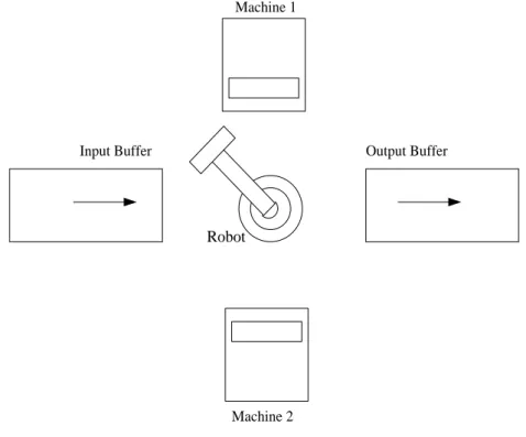
5.1 Robot centered cell layout . . . 68

6.1 Transition digraph . . . 76

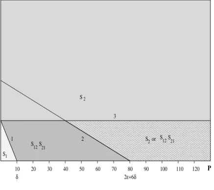
6.2 Regions of optimality for Example 6.2 . . . 91

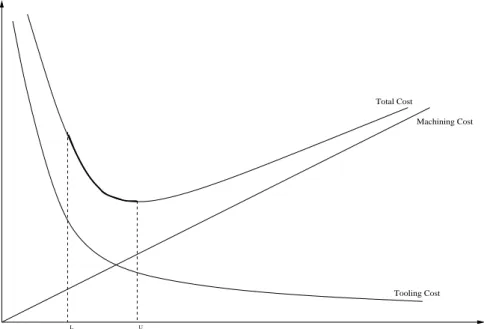
7.1 Manufacturing cost with respect to processing time . . . 98

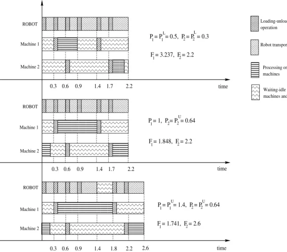
7.2 Gantt charts for different processing times for Example 7.1 . . . 110

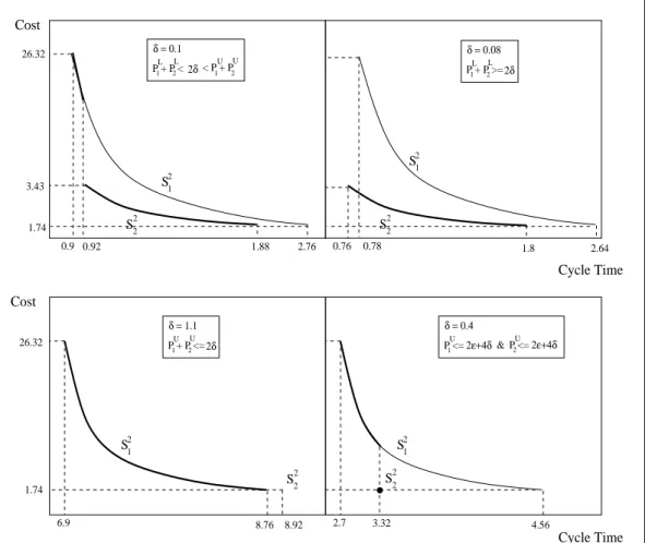
7.3 Different occurrences of the efficient frontier with respect to given parameters . . . 113

8.1 Comparison of points generated by the three methods . . . 163

8.2 Relative differences for 20 points with p = 20 . . . 169

LIST OF FIGURES _xv

8.3 CPU times for p = 20 operations with DICOPT . . . 170

8.4 CPU times for p = 20 operations with BARON . . . 171

List of Tables

8.1 Results of the first 5 iterations of EFFRONT-S2

2 and DICOPT

for Example 8.4 . . . 158

8.2 Experimental design factors . . . 160

8.3 Completion statistics for DICOPT and BARON . . . 162

8.4 Summary of results . . . 164

8.5 Paired t-tests . . . 166

8.6 Number of points generated by the EFFRONT-S2 2 and the CPU times . . . 167

8.7 Analysis of factors . . . 168

8.8 Comparison of EFFRONT with DICOPT with a multi-objective criteria . . . 173

G.1 Comparison of EFFRONT with DICOPT for 20 operations . . . 215

G.2 Comparison of EFFRONT with BARON for 20 operations . . . 216

G.3 Comparison of DICOPT with BARON for 20 operations . . . . 217

LIST OF TABLES _xvii

G.4 Comparison of EFFRONT with DICOPT for 50 operations . . . 218

G.5 Comparison of EFFRONT with DICOPT for 80 operations . . . 219

H.1 ANOVA tables for p = 20 operations . . . 221

Chapter 1

Introduction

The search for better ways to manufacture components has increased the level of automation in manufacturing industries. This trend involves the use of computer controlled machines and automated material handling devices. One of the widespread applications of automation is the installation and use of robotic cells. A manufacturing cell consisting of a number of machines and a material handling robot is called a robotic cell. These kinds of robots are used extensively in chemical, electronic and metal cutting industries. Robots are installed in order to reduce labor cost, to increase output, to provide a more flexible production system and to replace people working in dangerous or hazardous conditions [13]. However, in order to use such systems efficiently some important problems must be tackled. Among these, the design of the cells and the scheduling of robot moves are eminent.

In this thesis we will consider a flexible robotic manufacturing cell which consists of a number of Computer Numerically Controlled (CNC) machines and a material handling robot. “Flexibility” plays a crucial role in such cells. There are many different types of flexibilities such as operational flexibility,

CHAPTER 1. INTRODUCTION ₂

process flexibility, routing flexibility, material handling flexibility, and machine flexibility [18]. In this thesis we will consider those types of flexibilities that affect the processing times of the parts on the machines. More specifically, we will consider the operational and process flexibilities. Operational flexibility is defined as the capability of changing the ordering of several operations where process flexibility is defined as the capability of performing several operations at the same machine. Such flexibilities are achieved by considering alternative tool types for operations and loading multiple tools to the tool magazines of the machines.

We will investigate the productivity gain attained by the additional flexibility introduced by the CNCs. The aim is the maximization of the throughput of the cell or equivalently minimization of the cycle time which is defined as the long run average time required by the robotic cell to complete one part. More formally, we assume that we have infinite number of parts and if Cn denotes the completion time of the nth part then the long run average

cycle time is lim supn→∞Cn/n [21]. Cyclic production in a robotic cell refers to

the production of finished parts by repeating a fixed sequence of robot moves. As discussed in Geismar et al. [30], the main motivation for studying cyclic production comes from practice: cyclic schedules are easy to implement and control and are the primary ways of specifying the operation of a robotic cell in industry. Furthermore, Dawande et al. [23] show that for the problem of scheduling operations in bufferless robotic cells that produce identical parts (similar to our problem), it is sufficient to consider cyclic schedules in order to maximize throughput. They prove that there is at least one cyclic schedule in the set of all schedules that optimizes the throughput of the cell.

After reviewing the relevant literature in Chapter 2 we formulate our problem and present the necessary definitions and notation in Chapter 3. The focus of Chapter 4 is an m-machine robotic cell in which the machines are

CHAPTER 1. INTRODUCTION ₃

assumed to be capable of performing all the required operations of each part. As a consequence of this assumption, we relax the flowshop assumption which is used in the current literature and which unnecessarily limits the number of alternatives. The flexibility of the CNC machines leads to the definition of a new class of robot move cycles. We select and focus on one of the cycles among this class which is widely used in industry not because it is proved to be optimal but because it is simple and practical. The regions of optimality for this cycle for the m-machine case is determined. We analyze the 2- and 3-machine cases further in detail. For the regions where the proposed cycle may not be optimal, we present a worst case performance bound of using this cycle.

Till now the research on robotic cell scheduling problems concentrated on the operational aspects such as finding the part input sequence and the robot move sequence. However, the design of the cells also affects the performance of such cells. In Chapter 5, we study some design problems arising in robotic manufacturing cells. We first consider the layout of the machines and show that the efficiency of the cells can be increased by changing the layout of the machines. As a second design problem we consider the number of machines as a decision variable. We determine the optimal number of machines that minimizes the cycle time for given parameters such as the robot transportation time, load/unload time and the processing times of the operations.

Assuming that the CNC machines are capable of performing all the required operations may be unrealistic at times since the tool magazines have limited capacity and in many practical applications the required number of tools exceeds this capacity; ultimately, duplicating all the tools may not be economically justifiable. In this respect, in Chapter 6 we consider a 2-machine robotic cell and assume that some operations can only be processed on the first machine while some others can only be processed on the second machine

CHAPTER 1. INTRODUCTION ₄

due to tooling constraints. As a consequence, the system is assumed to be a flowshop in which each part passes through all machines in the same sequence; 1, 2, . . . , m. The remaining operations can be processed on either machine. The problem is to find the allocation of the remaining operations to the machines and the optimal robot move cycle that jointly minimize the cycle time. We prove that the optimal solution is either a 1-unit or a 2-unit robot move cycle, where an n-unit cycle is defined to be a cycle in which all machines are loaded and unloaded exactly n times and the initial and the final states of the system (position of the robot and the status of each machine) are the same. We present the regions of optimality for all 1-unit and 2-unit robot move cycles. Finally, a sensitivity analysis on the results is conducted.

Processing times of the parts on the machines can be changed by altering the machining conditions such as the speed and the feed rate for highly flexible CNC machines and this affects the cycle time. On the other hand, altering the machining conditions also affects the manufacturing cost. As a result, in Chapters 7 and 8 we develop and solve a bicriteria problem formulation for the robotic cell scheduling problem. In Chapter 7, we consider 2- and 3-machine robotic cells. The cell is assumed to be a flowshop in which each part has one specific operation on each machine and follows the same sequence of machines. The aim is to find the robot move sequence as well as the processing times of the parts on each machine that not only minimizes the cycle time but, for the first time in robotic cell scheduling literature, also minimizes the manufacturing cost. For each 1-unit cycle in 2- and 3-machine cells, we determine the efficient set of processing time vectors such that no other processing time vector gives both a smaller cycle time and a smaller cost value. We also compare these cycles with each other to determine the sufficient conditions under which each of the cycles dominates the rest. Finally, we show how different assumptions on cost structures affect the results. On the other hand, in Chapter 8, besides

CHAPTER 1. INTRODUCTION ₅

determining the robot move sequence and the processing times of the operations on the machines, we determine the allocation of the operations to the machines. Since finding the allocation of the operations is NP-Hard itself, we develop a heuristic algorithm which approximates a set of points on the efficient frontier. An experimental framework is designed in order to evaluate the efficiency of the algorithm and the results are compared with a commercial nonlinear mixed integer program solver software GAMS-DICOPT2x-C.

Chapter 2

Literature Review

In this section we will review the relevant literature pertinent to this study. However, let us first give some necessary notation and definitions that will be used throughout this study. The following definitions are borrowed from [19].

Definition 2.1 Ai is the robot activity defined as; robot unloads machine i,

transfers part from machine i to machine i + 1, loads machine i + 1.

Definition 2.2 An n-unit robot move cycle is the robot move cycle in which starting with an initial state of the system, the robot performs each activity exactly n times and ends up with the initial state of the system. Note that, in an n-unit robot move cycle exactly n parts are produced.

In an m-machine robotic cell we have exactly m + 1 robot activities: A0, A1,

. . ., Am, where the machines are numbered as 1, 2, . . . , m, the input buffer

is numbered as 0 and the output buffer is numbered as m + 1. Since in an optimal cycle we require that the robot move path is as short as possible, any two consecutive activities uniquely determine the robot moves between them.

CHAPTER 2. LITERATURE REVIEW ₇

Therefore, any robot move cycle can be uniquely described by a permutation of the above activities. Additionally, Crama et al. [21] make the following basic feasibility assumptions which we shall incorporate in our study as well:

1- Robot cannot load an already loaded machine. 2- Robot cannot unload an already unloaded machine.

These assumptions restrict the ordering of the activities. For example, let Sim

represent a specific robot move cycle in an m-machine robotic cell. Then for two machines we have only two feasible 1-unit robot move cycles:

S2

1 = A0A1A2, S22 = A0A2A1.

In a 3-machine cell there are six feasible 1-unit cycles which can be listed as follows:

S3

1 = (A0A1A2A3), S23 = (A0A2A1A3), S33 = (A0A1A3A2),

S3

4 = (A0A3A1A2), S53 = (A0A2A3A1), S63 = (A0A3A2A1).

The animated views of these robot move cycles can be found at the web site http://www.ie.bilkent.edu.tr/∼robot. Now, let us calculate the cycle time of S2

2 for a 2-machine cell producing identical parts as an example. Let Pi

represent the processing time of each of the identical parts on machine i and wi

represent the waiting time of the robot in front of machine i. Let TS represent

the cycle time of the robot move cycle S, i.e., the long run average time to produce one part under robot move cycle S. Furthermore, let δ represent the robot transportation time between any two consecutive machines and ² represent the loading/unloading time of the machines. In this cycle, initially

CHAPTER 2. LITERATURE REVIEW ₈

the first machine is idle and the second machine is loaded. The robot is in front of the input buffer just before taking a part. The robot takes a part from the input buffer (²), transports it to the first machine (δ), loads it (²), travels to the second machine (δ), waits in front of the machine to finish processing of the part (w2), unloads it (²), transports the part to output buffer (δ), drops the

part (²), travels back to the first machine (2δ), waits in front of the machine (w1), unloads it (²), transports the part to the second machine (δ), loads it (²),

travels back to input buffer (2δ). The initial and the final states are the same thus the cycle is completed. Then the cycle time is the following:

TS2

2 = 6² + 8δ + w1+ w2.

Note that, when the robot arrives in front of a machine to unload it, if the processing of the part is already completed then the robot unloads the machine immediately without any waiting time. Otherwise, the waiting time is equivalent to the remaining processing time. As a consequence, the waiting times are w1 = max{0, P1 − 2² − 4δ − w2} and w2 = max{0, P2− 2² − 4δ}.

After some simple arithmetic operations, the cycle time is found as follows:

T_S2

2 = 6² + 8δ + max{0, P1− 2² − 4δ, P2− 2² − 4δ}.

Now let us consider the basic assumptions that are common for most of the studies.

• All data are deterministic.

• The robot and the processing machines never experience breakdown and never require maintenance. Setup times are assumed to be negligible. • No preemption is allowed in the processing of any operation.

CHAPTER 2. LITERATURE REVIEW ₉

• Parts are always available at the input buffer and there is always an empty place at the output buffer.

In the next section we will list the differences in robotic cell scheduling problems and present the standard classification scheme for those problems. In Section 2.2, we will present basic results from the previous studies on robotic cell scheduling problems. In Section 2.3, the multicriteria scheduling models considered in FMS scheduling literature are explained. The studies considering controllable processing times in scheduling are summarized in Section 2.4.

2.1

Problem Types and Classification Scheme

The robotic cell scheduling problems differ from each other in the following aspects:

1. Cell types,

2. Processing times, 3. Objective functions, 4. Robot travel times,

5. Loading and unloading times, 6. Number of machines and parts.

CHAPTER 2. LITERATURE REVIEW ₁₀

2.1.1

Cell types

In most general terms, a robotic cell consists of m machines denoted as Mi, i =

1, 2, . . . , m. Also there is an input and an output buffer denoted as (M0)

and (Mm+1) respectively. In some implementations, the input device and the

output device are at the same location, and this unit is called a load lock [30]. In most studies there is one robot that makes the loading/unloading of the machines and the transportation of the parts between these machines. Some studies also consider the multiple robots case.

An important characteristic of the robotic cells is the buffers in front of the machines. In the literature, robotic cells with finite or infinite buffers and no buffers are considered. In general, the additional freedom introduced by buffers tends to complicate scheduling problems [82]. The focus of this study is on robotic cells with no buffers. For the complexity of the robotic cells with buffers we refer to Hurink and Knust [51]. Other problems and approaches to this subject can be found in Kise [65], Hitomi and Yashimura [49], King et al. [64], Finke et al. [27], Levner [71], and Kogan and Levner [66].

For the bufferless problems, all parts must be either on the input buffer, on one of the machines, on the output buffer, or on the robot. This is equivalent to blocking condition in a classical flowshop: a part that has completed processing on Mi can not leave unless machine Mi+1 is unoccupied [83]. This should not

be confused with the more restrictive no-wait condition in which a part must be removed from a machine and transferred to the next one as soon as that first machine completes processing that part, a condition which will be analyzed in Section 2.1.2.

Some researchers consider cells with dual gripper robots instead of single gripper robots. Dual gripper robots can hold two parts at a time and unload

CHAPTER 2. LITERATURE REVIEW ₁₁

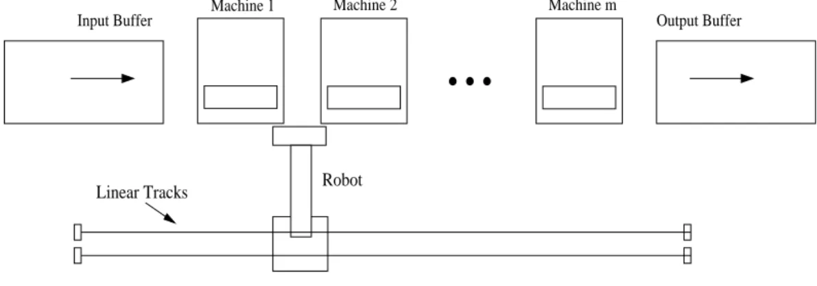
Linear Tracks Robot

Input Buffer Machine 1 Machine 2 Machine m Output Buffer

...

Figure 2.1: Inline robotic cell layout

and load a machine simultaneously. This increases the number of feasible robot move cycles drastically. As a consequence, the complexity of the problem also increases. Another stream of research considers parallel machines at each stage of production. The robot makes the transportation between the stages and the loading/unloading of the parallel machines is performed by another material handling device.

Another characteristic of the robotic cells is the layout of the cells. As Han et al. [47] proposed, cell formation may increase efficiency of the cell. Three different layouts are considered for the robotic cells: robot-centered cells denoted as RCCm for an m-machine robotic cell, (where the robot movement is rotational), in-line robotic cells denoted as IRCm (where the robot moves linearly) and mobile-robot cells denoted as MRCm (generalization of in-line robotic cell and robot-centered cell) [75]. In this thesis, consistent with most of the research on this area, we will assume an in-line robotic cell layout as shown in Figure 2.1.

CHAPTER 2. LITERATURE REVIEW ₁₂

2.1.2

Processing times

In most general terms, the processing times are represented as [Lj_i, U_ij] which gives the processing time of part j on machine Mi. The meaning of the

processing window is that the time spent by part j on machine Mi must be

at least Lji and may not exceed Uij. For example, if we consider the case that

each part has a precisely defined processing time on each machine and can wait on the machine indefinitely long after it has been processed, it can be handled by setting all upper bounds U_ij to +_{∞. This case is referred to as} unbounded processing windows [21]. Another type of processing requirement is referred to as with blocking, i.e., the machine becomes blocked if the part is not removed from it after the processing is finished. Another model is referred to as no-wait; here it is assumed that the parts must be removed from the machines immediately after the processing is finished. These two problems can be modelled by setting Lj_i = U_ij. This setting of processing windows is referred to as zero-width processing windows [21]. No-wait type processes are commonly seen in chemical and electronic industries, where the parts are dipped into chemical substances, after a certain amount of time taken out and in order not to become defective should immediately proceed with the next operation in sequence. Also in plastic molding and steel manufacturing, where the raw material must maintain a certain temperature, no-wait type conditions are used. Such conditions also ensure freshness in food canning industries (Hall and Sriskandarajah [46]). There is vast amount of research focusing on these types of problems.

Another problem with a different processing requirement is formulated in Akturk et al. [2] and Gultekin et al. [38] where the processing times are assumed to be decision variables. The parts are assumed to have several operations to complete their processing. Each operation has its own operation

CHAPTER 2. LITERATURE REVIEW ₁₃

time. Then these operations are tried to be allocated to the machines in order to minimize the cycle time. Thus, the processing times depend on the allocation of the operations.

2.1.3

Objective functions

There are two objective functions that are commonly used in robotic cell scheduling literature. The first and the most widely used one is the minimization of the cycle time or the maximization of the throughput. Since the robot follows a computer program, there must be a finite activity sequence for the robot that it repeats to produce the parts. Thus, the robot activities must be cyclic because of its nature and minimizing this cycle time is a relevant objective. Cycle time is defined as the long run average time that is required to produce one part where each robot activity is performed an equal number of times and the initial and the final states of the system are the same. The cycle time for an n-unit cycle is found by dividing the total time required to finish the cycle by n so that the average time to produce one part is found. The second objective function that is used widely is the minimization of the makespan of the schedule, which is defined as the completion time of the last job in the sequence.

2.1.4

Robot travel times

In the most general case, robot travel time between machine i and j is assigned a value δij, 0≤ i, j ≤ m+1. The travel times are neither additive nor constant.

By additive we mean that δij = δi(i+1)+ δ(i+1)(i+2)+ . . . + δ(j−1)(j). That is, total

time to travel between machine i to machine j is the summation of the travel times between consecutive machines on the way from machine i to machine j.

CHAPTER 2. LITERATURE REVIEW ₁₄

Brauner et al. [11] study this problem with the following assumptions:

1. The travel time from a machine to itself is zero, i.e., δii = 0,∀i.

2. The travel times satisfy the triangular inequality, i.e. δij + δjk ≥ δik,

∀i, j, k.

3. The travel times are symmetric, i.e. δij = δji, ∀i, j.

A robotic cell that satisfies Assumptions 1 and 2 is called a Euclidean robotic cell; one that satisfies Assumptions 1,2 and 3 is called a Euclidean symmetric robotic cell [30]. The robotic cell scheduling problem for either case is NP-hard in the strong sense [11].

In some studies, the robot travel time is assumed to be additive and constant for any transportation between any two consecutive workstations in which case δij = δ ∀i, j.

In more realistic cases, the acceleration and the deceleration of the robot is considered [75]. In this case, the travel time between two consecutive machines does not change while on the other hand, the travel time between non-consecutive machines is reduced. For each intervening machine, the robot is assumed to save γ units of time.

For mobile robot cells, since the robot both moves linearly and rotationally, the linear movement can take more time. For a two machine cell this occurs when the robot moves between machines 1 and 2 [75]. Thus, a time denoted δ0 is added to the travel time for the movements that include transportation

between machines 1 and 2.

Dawande et al. [24] consider another transportation time model in which additivity is not applicable. They assume that the robot travel time between

CHAPTER 2. LITERATURE REVIEW ₁₅

any pair of machines is constant δ. This happens when the cells are compact and the robots have varying acceleration and deceleration. Thus, the travel times between any pair of machines vary in negligible amounts.

2.1.5

Loading and unloading times

Several authors consider the loading and unloading times to be machine dependent, that is, it takes ²i time to load or unload a part to machine i.

In other cases, this time is assumed to be constant for all workstations and parts that is, ²i = ²,∀i. Dawande et al. [24] state that, when comparing cycle

times of different cycles, the values of ²i has no effect. This is because no

matter what the robot’s sequence may be, each part is unloaded from input buffer, loaded and unloaded on each machine and loaded on output buffer.

2.1.6

Number of machines and parts

In a robotic cell the number of machines may differ from 2 to m. Naturally most analytical results are for the cases where the number of machines are relatively small, namely two and three. For the cases where the machine number is more than three, most of the problems appear to be NP-hard. However, when a flexible robotic cell is considered which consists of CNC machines, the number of machines is relatively small due to physical space constraints.

The number of parts considered may also differ among the existing studies in the literature. Some of the studies assume identical parts for which there is no sequencing of the parts. The only problem is to find the robot move cycle that minimizes the cycle time. On the other hand, in multiple parts case the problem is to find the robot move sequence as well as the part input sequence

CHAPTER 2. LITERATURE REVIEW ₁₆

that jointly minimize the cycle time. It is obvious that this problem is much more difficult than its identical parts counterpart and most of the analytical results derived for the identical parts case fail to apply to this case. Again, because of the nature of industrial robots, the multiple parts case also must follow a cycle and this cycle can use the concept of minimal part set (MPS). The MPS for a production environment can be obtained, if the forecasted demand Lj is given for each part type j over planning horizon. If d is the largest

common divisor of the integers L1, L2, . . . , Lk, the integer ratio (rj = Lj/d) of

part types can be represented as r = (r1, r2, . . . , rk). The vector is the minimal

production ratio (MPR) and the part set corresponding to this ratio is known as the MPS. For the sake of clarity consider the following example. Let us assume that we have three products A, B and C, with forecasted demand, Lj,

being 100, 150 and 250 respectively. Then, the largest common divisor, d, is 50 and the MPR is (2, 3, 5). As a result, the MPS is composed of 2 A’s, 3 B’s and 5 C’s. Given an MPS of n parts, Geismar et al. [30] define an MPS cycle to be a sequence of robot moves in which exactly n parts of an MPS enter the cell at the input station, exactly n parts of the MPS exit the cell at the output station and the cell returns to its initial state. The order in which the parts enter the cell is called the MPS part schedule (or simply part schedule). An MPS cycle is determined by the MPS part schedule and the MPS robot move sequence or simply robot move sequence that specifies all robot operations during the MPS cycle. Sriskandarajah et al. [89] define Concatenated Robot Move Sequences (CRM Sequences) as a class of MPS cycles in which the same 1-unit cycle of robot actions are repeated n times. Thus, the problem in multiple parts case is to find the robot move sequence and the part input sequence of the MPS.

Now let us present the classification scheme for robotic flowshops, which will help us through the rest of this study. The standard classification scheme for scheduling problems introduced by Graham et al. [36] can be denoted as

CHAPTER 2. LITERATURE REVIEW ₁₇

ψ1|ψ2|ψ3 where ψ1 indicates the scheduling environment, ψ2 indicates the job

characteristics or restrictive requirements and ψ3 defines the objective function

to be minimized. Hall et al. [43] extended this scheme to capture the scheduling problems arising in robotic cells, as follows:

Under ψ1, we have:

M RCm = a mobile-robot cell with m machines. RCCm = a robot-centered cell with m machines. IRCm = an in-line robot cell with m machines.

Under ψ2, we have:

k = the number of part-types.

r-unit(s) = the problem is being solved over robot move cycles that produce r units.

S = robot move cycle S is used alone.

δi = δ = the travel time between any pair of consecutive machines

is equal.

²i = ² = the load and unload times at all machines are equal.

Under ψ3, we have:

Ct = long run average time to produce one part.

Cmax = the makespan for the manufacture of a given set of jobs.

In the next section, we will present basic results of the previous research on robotic cell scheduling problems.

CHAPTER 2. LITERATURE REVIEW ₁₈

2.2

Results from Previous Studies

There is vast amount of research on robotic cell scheduling problems. Some date as far as 1970s, but the majority has been performed since 1990. We will analyze the results from previous studies under the headings of identical parts case, multiple parts case and some other cell configurations that have particular assumptions. Crama et al. [21], Lee et al. [69] and Geismar et al. [30] also provide surveys in this area.

2.2.1

Identical Parts Case

The identical parts robotic cell scheduling problem is simpler than its multiple parts counterpart since the part sequencing problem vanishes in identical parts case. However, like most scheduling problems, analytical results are found for problems where there the number of machines is small.

The paper by Sethi et al. [86] can be considered as the initiation of the robotic cell scheduling literature. In this study, the objective is to maximize the throughput or in other words minimize the cycle time. One of the problems considered in this study is ”one part type problem with two machines”, more specifically, RCC2_{|k = 1, δ}i = δ, ²i = ²|Ct. For this problem they prove that the

optimal solution is a 1-unit cycle. Since there are a total of two feasible 1-unit cycles in a 2-machine cell, they determine the regions of optimality for each of these cycles by comparing the cycle times of these two cycles with each other. Another problem considered in the paper is “one part type problem with three machines”, that is, RCC3|k = 1, δi = δ, ²i = ², 1− unit|Ct. Determining the

sequence of robot moves constituting a 1-unit cycle that minimizes the cycle time is considered. In this problem, only 1-unit cycles are considered since the analysis of the problem without this restriction is difficult and perhaps

CHAPTER 2. LITERATURE REVIEW ₁₉

intractable. As a solution to this problem, a decision tree is constructed in order to determine the optimal policy. It is also proved that the number of one-part cycles in the m-machine case is exactly m!. Another important result of the paper is the conjecture that optimal 1-unit cycles are superior to every n-unit cycle, for n_{≥ 2.}

Crama et al. [19] consider the problem RCCm_{|k = 1, δ}i, ²i, 1− unit|Ct.

They show that, when there is only one type of part to be produced and considering only 1-unit cycles, the problem can be solved in (strongly) polynomial time, even if the number of machines is viewed as an input parameter of the problem. This generalizes previous results established by Sethi et al. [86]. This result is achieved by proving that the set of pyramidal permutations necessarily contains an optimal solution of the problem. Pyramidal permutations have been previously introduced in the framework of the travelling salesman problem; see e.g. Gilmore et al. [35]. Let π = (A0, Ai1, . . . , Aik, Aik+1, . . . , Aim). Then, π is pyramidal if 1 ≤ i1 <

. . . < ik = m and m > ik+1 > . . . > im ≥ 1. An algorithm is given which

computes the cycle time of a schedule described by a pyramidal permutation. Lastly, a dynamic programming approach is presented that solves the identical parts cyclic scheduling problem with the restriction that one unit is produced in each cycle in O(m3_{) time where m is the number of machines in the cell.}

Another result of that study is the derivation of the upper and the lower bounds on the optimal cycle time.

Hall et al. [43] consider 3-machine cells producing single part-types and prove that, the repetition of 1-unit cycles dominates more complicated policies that produce two units. The validity of the conjecture of Sethi et al. [86] for 3-machine robotic flowshops is established by Crama et al. [20]. Brauner and Finke [9] simplify this proof. In a later study, Brauner et al. [10] prove that 1-unit cycles do not necessarily yield optimal solutions for cells of size four or

CHAPTER 2. LITERATURE REVIEW ₂₀

large. They present examples of such cases.

Dawande et al. [24] consider a different case of identical parts robotic cell scheduling problem. They study the problem of finding the optimal robot move cycle that minimizes the cycle time in an m machine robotic cell. However, they consider only the 1-unit cycles. Differing from the literature, they assume that the robot travel time between any pair of machines is constant, which is referred to as constant travel time robotic cells. Such cells are used in some manufacturing systems such as manufacturing of wafers. They provide a polynomial time algorithm for finding an optimal 1-unit cycle.

Dawande et al. [23] show that cyclic schedules which repeat a fixed sequence of robot moves indefinitely are the only ones that need to be considered in order to maximize the long-term average throughput. Additionally, for the different classes of robotic cells studied in the literature, the authors discuss the current state of knowledge with respect to cyclic schedules. Geismar et al. [29] consider an m-machine flexible robotic cell. They assume that each part has one operation to be performed on each machine which makes a total of m operations. They also assume that each part visits the machine in the same order. However, the operations can be performed in any order and each machine can be configured to perform any operation. They try to determine the assignment of the operations to the machines so that the throughput is maximized. They consider both the cases where the assignment of the operations remains the same throughout the processing of the lot and it varies for successive parts within a processing lot for 2, 3 and 4-machine cells.

A considerable amount of research in robotic cell scheduling area considers the no-wait constraints which are required in some manufacturing systems such as plastic molding, electroplating and steel manufacturing. In these systems, material handling is mainly done by an automated material handling device

CHAPTER 2. LITERATURE REVIEW ₂₁

such as AGV’s, hoists or robots. There is a vast amount of literature on no-wait constraints in hoist and AGV scheduling problem areas. Since AGV scheduling, hoist scheduling and robotic cell scheduling problems can be considered as special cases of one another, the results for one of them can be extended to be used for another, For example a single loop, single hoist scheduling problem can be considered as a robotic cell scheduling problem.

One such study with no-wait constraints is the study of Kats et al. [61]. They consider an m machines identical parts robotic cell scheduling problem with the objective of finding the 1-unit robot move cycle that minimizes the cycle time. They assume that any machine may occur more than once in the processing sequence of the parts. A polynomial algorithm which solves the problem in O(K5) is presented. Here K is the number of processing stages in the part’s production. If the re-entrance constraint is relaxed, they show that the same algorithm has complexity O(m4), where m is the number of machines. In a later study, Levner et al. [70] consider the same problem without re-entrance constraints. They present an algorithm which in turn improves the complexity of the previous one to O(m3_{log m).}

In a most recent study in no-wait robotic cells, Che et al. [15] consider an m machine robotic cell with identical parts and constant processing times. The objective is to find the optimal 2-unit robot move cycle that minimizes the cycle time. They propose an algorithm which solves the problem in O(m8_{log m)}

time. They also extend this algorithm for the case of two nonidentical parts. They present computational results which show that the algorithm effectively finds the 2-unit cycles that minimizes the cycle time.

CHAPTER 2. LITERATURE REVIEW ₂₂

2.2.2

Multiple Parts Case

As already mentioned, multiple parts problems are harder than the identical parts problem even for small number of machines. Recall that, the problem is to find the robot move sequence and the part input sequence for the MPS that jointly minimize the cycle time.

In their study, Sethi et al. [86] consider multiple parts case also. More specifically they consider RCC2|k ≥ 2, δi = δ, ²i = ², S12(S22)|Ct. Given a fixed

sequence for the robot moves in a 2-machine cell and the desired production ratios of the part types to be produced (MPS), determining the schedule of parts at the input station that minimizes the cycle time is considered. As a solution to this problem a polynomial time algorithm that determines an optimal multi-part cycle is proposed.

Kise et al. [65] consider 2-machine multiple parts problem with the objective of minimizing the makespan. They propose an O(n3_{) procedure}

that solves the problem based on the known Gilmore and Gomory algorithm (Gilmore and Gomory [34]). For the same problem, if the transportation time between the machines is job dependent, then the problem is equivalent to an asymmetric travelling salesman problem and is NP-hard in the strong sense (Stern and Vitner [91]).

Again for the 2-machine multiple parts problem, Logendran and Sriskan-darajah [75] consider three different layouts and establish optimal robot sequences for these layouts. The problem of determining the optimal sequence of multiple part types is shown to be equivalent with a 2-machines no-wait flow shop problem, and is solved by Gilmore and Gomory’s algorithm. Besides the analysis of a single MPS, production of multiple MPSs is also analyzed.

CHAPTER 2. LITERATURE REVIEW ₂₃

problems simultaneously. They consider M RC2_{|k ≥ 2, δ}i = δ, ²i = ²,|Ct.

They prove that CRM sequences generally do not give the optimal MPS robot move sequences and they provide an example depicting this situation. An O(n4_{) algorithm is provided for this case which gives the robot move cycle}

and part input sequence that jointly minimize the cycle time, where n is the number of parts in the MPS. They also consider the problem M RC3|k ≥ 2, δi = δ, ²i = ², S13(S23, S33, S43, S53, S63)|Ct. They show that the optimal part

sequencing problems associated with 4 of the 6 potentially optimal robot move cycles for producing 1-unit are polynomially solvable and for the remaining 2 cycles, they show that the recognition version of the part sequencing problem is NP-complete. More specifically, they show that the optimal part schedule based on S3

1 is trivially solvable whereas the optimal part schedule based on

S3

3, S43 and S53 can be solved polynomially using an algorithm based on the

Gilmore-Gomory [34] algorithm. On the other hand, finding the optimal part schedules for S3

2 and S63 are NP-hard. Also, the conditions on the relative

lengths of processing times compared to robot move times under which the last 2 cycles are dominated by the other 4 are given.

Aneja et al. [5] also consider M RC2|k ≥ 2, δi = δ, ²i = ²,|Ct like Hall et al.

[43] and improve their algorithm which finds the optimal robot move sequence and the part input sequence. They model the problem as a special case of TSP and provide an algorithm of complexity O(n log n).

Sriskandarajah et. al. [90] consider M RCm_{|k ≥ 2, δ}i, ²i|Ct. They classify

1-unit robot move cycles in an m-machine cell, for m _{≥ 2, according to the} tractability of their associated part sequencing problems. The classification is as follows:

U : Sequence independent (trivially solvable),

CHAPTER 2. LITERATURE REVIEW ₂₄

V2 : Unary NP-hard TSP models,

W : Unary NP-hard, but not having TSP structure.

As a consequence of this classification, it is proved that the part sequencing problems associated with exactly 2m− 2 of the m! available robot cycles are polynomially solvable. The remaining cycles have associated part sequencing problems which are unary NP-hard.

Another important result of the paper is as follows: in an m-machine robotic cell with m≥ 4 there are m! robot move cycles of which:

(a) One U-cycle defines a trivially solvable part sequencing problem,

(b) 2m_{− 3, V1-cycles define a part sequencing problem which is solvable in} O(nlogn) time, (c) bm/2cP t=1 ³_m 2t ´

−2m+3, V2-cycles define a part sequencing problem which can be formulated as a TSP and which is unary NP-hard.

(d) m!_{− 1 −}bm/2cP

t=1

³_m

2t

´

, W-cycles define a part sequencing problem which in general cannot be formulated as a TSP, and which is unary NP-hard.

Hall et al. [44] consider a 3-machine cell which produces multiple part-types and prove that in two out of six potentially optimal robot move cycles for producing one unit, the recognition version of the part sequencing problem is unary NP-complete. The intractability of the part sequencing problem not restricted to any one-unit cycle, that is, M RC3|k ≥ 2, δi, ²i|Ct, is also proved.

Lastly, an algorithm is provided which initializes an empty cell into a steady state as quickly as possible for any potentially optimal one-unit cycle.

Kamoun et al. [56] consider various problems in multiple parts scheduling case and design and test heuristic procedures for the part sequencing problem.

CHAPTER 2. LITERATURE REVIEW ₂₅

They provide heuristics for the following problems: M RC3_{|k ≥ 2, δ}i, ²i, S23|Ct

and M RC3|k ≥ 2, δi, ²i, S63|Ct which were shown to be NP-hard by Hall et

al. [43]. They also consider the most general 3-machine case, M RC3_{|k ≥} 2, δi, ²i|Ct, in which all possible robot move cycles are considered. Hall et

al. [44] prove that its recognition version is unary NP-complete. An efficient heuristic is defined and tested for this problem also. The ways of extending these heuristics to four machine cells as well as larger cells are illustrated. They also consider a cell design problem which involves organizing several machines into R _{≥ 2 cells, which are arranged in a serial production process} with intermediate buffers.

Agnetis [1] consider a multiple parts no-wait robotic cell scheduling problem with m machines. They assume that the parts are grouped into lots of identical parts. They propose an ε-approximate algorithm which is based on the solution to a transportation problem. Computational analysis results are presented.

2.2.3

Other Cell configurations

A new area of research is focusing on the robotic cells served by a robot with a dual gripper. These robots are considered as a means to increase throughput. These types of robots can hold two parts simultaneously and thus, make it possible to unload a part from a machine and load it with another part at the same time. This ability results in a huge increase in the number of possible robot move cycles. For such robots, another time called the repositioning time is defined. This is the required time to reposition the second gripper of the robot in front of the machine after the first gripper finishes its loading/unloading operation. It is generally assumed that the repositioning requires much less time than the robot’s movement between two adjacent machines or any machine’s processing time [30].

CHAPTER 2. LITERATURE REVIEW ₂₆

Droboutchevitch et al. [26] consider identical parts case and develop a formula to find the number of nondominated cycles in a general cell with m machines. They show that for m = 2 there are 52 feasible 1-unit cycles. However, they show that 13 of them dominate the rest.

Sethi et al. [85] also consider the dual gripper robotic cell scheduling problem with identical parts and m machines. Since this problem is much more complex than the case of single gripper robotic cell scheduling problem, they extend the existing analytical framework to develop all 1-unit cycles for dual gripper robotic cells. They consider only the 1-unit robot move cycles and examine the cycle time advantage (or productivity advantage) of using a dual gripper robotic cell rather than a single gripper robot. The best possible improvement achieved by implementing a dual gripper robot appears to be reducing the cycle time by half. They also propose a practical heuristic algorithm to compare productivity of a single gripper and a dual gripper for given cell data. Conditions which indicate the use of a dual gripper robot include [30]:

1. m is not large and maxi{Pi/(δ + 2²)} is large.

2. m is large and maxi{Pi/(δ + 2²)} is not large.

3. ²/δ _{≤ 1.}

Sriskandarajah et al. [89] consider dual gripper robotic cells with multiple parts. Focusing only on CRM sequences, they develop the notational and modelling framework for cyclic production of multiple parts in dual gripper robotic cells. They demonstrate that the recognition version of the part sequencing problem subject to a given robot move sequence is unary NP-complete for 6 out of 13 undominated sequences. For the special case of negligible gripper switching time, they identify the robot move sequence that

CHAPTER 2. LITERATURE REVIEW ₂₇

gives the minimum cycle time. For the general case, they provide an efficient heuristic, which is empirically tested. Also computational experiments are made to study the productivity gains of using a dual gripper robot in place of a single gripper. They find the mean relative improvement range between 18% and 36%.

Drobouchevitch et al. [25] also consider dual gripper robotic cells with multiple parts. They consider 2-machines case. They focus on the intractable problem of parts sequencing in a 2-machine dual gripper robot cell. They develop a heuristic based on Gilmore-Gomory [34] that provides 3/2-approximation of the optimum for the 6 NP-hard CRM sequences. A linear program is used to establish the performance guarantee without actually calculating a lower bound. This approach is original in the literature of scheduling robotic cells.

There are many other interesting robotic cell configurations in the literature. An important class of problems addresses robotic cells involving more than one robot. Problems of this type can be found in Karzanov and Livshits [59] and Lieberman and Turksen [73]. In one of such problems Kats et al. [60] study the problem of m machines identical parts no-wait robotic cell scheduling problem with the objective of minimizing the number of robots required to meet a cycle time of T . They propose an O(m5_{) time algorithm}

that solves the problem optimally. Also in another study, Kats and Levner [62] consider minimization of cycle time over the 1-unit robot move cycles with the no-wait constraint and identical parts. They solve the problem for single and several robots. They assume that the set of machines served by each robot is known in advance. They solve the problem in O(m3_{logm) time. They also}

show that the cyclic multi-robotic problem of the paper can be interpreted as a new polynomially solvable case of the cyclic no-robot job-shop scheduling problem.

CHAPTER 2. LITERATURE REVIEW ₂₈

A special case of robotic cell scheduling is when all of the machines are identical and working in parallel. Hall et al. [45] consider these systems with different objectives (e.g. makespan, Cmax; maximum lateness, Lmax;

total tardiness, P

Tj etc.) and derive complexity results for these problems.

Geismar et al. [31] consider identical parts, parallel machines robotic cell where the robot travel time is assumed to be constant for any pair of machines. The authors provide guidelines to determine whether parallel machines will be cost-effective for a given implementation. They also provide a simple formula for determining how many copies of each machine are required to meet a particular throughput rate and an optimal sequence of robot moves for a cell with parallel machines under a certain common condition on the processing times.

Geismar et al. [32] combine dual gripper robotic cells and robotic cells with parallel machines. The robot travel time is assumed to be constant for any pair of machines. They provide a structural analysis of cells with one or more machines per processing stage to obtain first a lower bound on the throughput and subsequently an optimal solution under specific conditions. In another study, Geismar et al. [33] consider a parallel machine robotic cell with multiple robots that is used by a semiconductor equipment manufacturer. The travel times are assumed to be Euclidean. The authors describe a schedule of robot moves that is optimal under a common set of conditions for large cells containing multiple robots. When this set of conditions does not hold, even though optimality could not be proven, this schedule is shown to be superior to one currently in use by some semiconductor manufacturers. They also present a scheme that allows the robots to operate concurrently, efficiently, and with no risk of colliding.

Blazewicz et al. [8] consider a two-stage FMS, in which they assume limited buffers between the machines. A specific assumption of this problem was that some parts need additional operation so will leave the system after the first

CHAPTER 2. LITERATURE REVIEW ₂₉

machine and turn back later. Another difference of this research is that, they consider setup times and assume that the production is made with batches of identical parts. They also consider release dates of the parts and provide heuristics to minimize the makespan.

Some studies in this area consider different objective functions other than minimizing the makespan or the cycle time. For instance, Song et. al. [88] and Jeng et. al. [55] try to minimize the sum of completion times. On the other hand Levner and Vlach [72] consider an objective which minimizes some penalty function of the maximum lateness.

Hurink and Knust [52] consider a single machine scheduling problem which arises as a subproblem in a jobshop environment where the jobs have to be transported between the machines by a single transport robot. They present a tabu search algorithm for this problem, where they consider it as a generalized TSP.

Lastly, Han and Cook [47], develop a mathematical model and a solution algorithm for solving a robot acquisition and cell formation problem. They formulate the problem as a multi-type two-dimensional bin packing problem, which is known to be NP-hard. They develop and implement a heuristic algorithm. The computational results show that the problems can be solved with an optimality gap of less than 1% and over 70% of all solutions (334 out of 450) were optimal.

2.3

Multicriteria scheduling

A single criterion is used in most of the existing scheduling studies. Algorithms which focus entirely on optimizing one criterion may perform poorly for others

CHAPTER 2. LITERATURE REVIEW ₃₀

since most of the criteria are conflicting with each other. The trade-offs involved in considering several different criteria provide useful insights to the decision maker. For example, a solution which minimizes the cycle time (long run average time to produce one part) may perform poorly in terms of cost. Thus, in the context of real life scheduling problems it is more relevant to consider problems with more than one criterion. Multicriteria and bicriteria scheduling models can be reviewed from Hoogeveen [50] and Nagar et al. [78]. Multicriteria scheduling can provide good solutions for more than one objective. There are different ways to deal with multiple criteria. One way is combining objectives with linear, quadratic and Tchebycheff functions by assigning weights to each objective. Another way is finding efficient solutions which provide more than one alternative to the decision maker.

In multi-objective optimization problems, approximation quality of the generated efficient set is important to the decision maker. In the literature, there are different approximation quality evaluation metrics developed. These metrics are useful for comparing different algorithms. A review and discussion on existing metrics is available in Zitzler et al. [100]. Wu and Azarm [98] propose some quality evaluation measures to compare efficient sets generated by different multi-objective optimization methods.

The most common objectives used in multicriteria scheduling models are minimizing flow time, number of tardy jobs, maximum tardiness, total tardiness and total earliness. Koktener and Koksalan [68] use simulated annealing and Koksalan and Keha [67] use genetic algorithms to solve a bicriteria scheduling problem on a single machine. Ruiz-Torres et al. [84] study the bicriteria identical parallel machine scheduling problem with the objectives of minimizing the number of late jobs and minimizing the average flow time. A simulated annealing procedure is proposed to generate nondominated solutions. Suresh and Chaudhuri [92] propose a tabu search algorithm to solve bicriteria

CHAPTER 2. LITERATURE REVIEW ₃₁

scheduling problem for unrelated parallel machines with the objectives of minimizing the makespan and minimizing the maximum tardiness. Mohri et al. [76] solve the bicriteria scheduling problem on three identical parallel machines. The tradeoff curve which minimizes the makespan and maximum lateness is found. Tiwari and Vidyarthi [93] propose a genetic algorithm to solve machine loading problem with the availability of machining time and tool slots constraints. The objectives are minimizing the system unbalance and maximizing the throughput, which are the most commonly used objectives in FMS scheduling with multiple machines. Bernardo and Lin [6] consider the nonidentical parallel machine scheduling problem with the objectives of minimizing the total tardiness and minimizing the setup costs. Gupta and Ruiz-Torres [42] consider the objectives of minimizing total flow time and minimizing total number of tardy jobs simultaneously and propose heuristic algorithms to generate efficient solutions. Gupta and Ho [41] provide solution methods for the problem of minimizing makespan subject to minimum flow time for two parallel machines. Cao et al. [14] consider the machine selection and scheduling decisions together in order to minimize the sum of machine cost and job tardiness. Alagoz and Azizoglu [3] study a problem with the objectives of minimizing total completion time and minimizing number of disrupted jobs in a rescheduling environment.

Although, the local search heuristics do not guarantee to find all efficient solutions, they can find approximately efficient solutions for multiple criteria in reasonable computation times.

CHAPTER 2. LITERATURE REVIEW ₃₂

2.4

Controllable Processing Times

In robotic cells, highly flexible Computer Numerical Control (CNC) machines are used for the metal cutting operations so that the machines and the robot can interact in real time. Machining conditions such as the cutting speed and the feed rate are controllable variables for these machines. Consequently, the processing time of any operation on these machines can be reduced by changing the machining conditions at the expense of incurring extra cost resulting in the opportunity of reducing the cycle time. Due to this reasoning, assuming the processing times to be fixed on each machine is not realistic.

The first studies considering controllable processing times in scheduling problems are by Vickson [95], [96]. He considers the single machine problem with average flow cost and maximum tardiness objectives together with the total compression cost. The total compression cost is assumed to be a linear function of the processing time. An assignment model is proposed for the average flow cost objective. An algorithm is proposed for the maximum tardiness problem. Most of the studies consider single machine scheduling problems with linear compression cost functions (Panwalkar and Rajagopalan [81], Van Wassenhove and Baker [97], Daniels and Sarin [22]). Although this assumption simplifies the problem, it is not realistic in most cases because it does not reflect the law of diminishing returns. Nowicki and Zdrzalka [79] provide a survey for sequencing problems with controllable processing times which have a linear cost function. Mukhopadhyay and Sahu [77] consider the minimization of makespan as a primary objective and the minimization of the machining costs as a secondary objective.

There are few studies considering multiple machine problems. Zhang at al. [99] propose a 3/2-approximation algorithm for solving the unrelated parallel machine scheduling problem with the objectives of minimizing the

CHAPTER 2. LITERATURE REVIEW ₃₃

total weighted completion time and the processing cost. Ishii et al. [53] consider the uniform parallel machine scheduling problem with preemption. They propose polynomial time algorithms in order to find optimal speeds of the processors with the completion time and the processing costs objectives. Nowicki and Zdrzalka [80] consider parallel machine scheduling with completion time and processing cost objectives (preemption allowed). A greedy algorithm is proposed to find the efficient frontier for identical machines. An algorithm is proposed for the uniform machine case in order to find the ²-approximation of the efficient frontier. Trick [94] proposes an integer programming formulation and a heuristic to solve the multiple capacitated machine problem with makespan objective.

The minimization of earliness and tardiness objective is considered in a few number of papers considering controllable processing times. Most of them consider the common due date assumption. Panwalkar and Rajagopalan [81] consider a single machine problem with controllable processing times. The objective is minimizing the sum of earliness and tardiness penalties and total processing costs. The common due date is a decision variable that should be determined with the proposed assignment model. Liman et al. [74] replace the common due date assumption with the common due window assumption. They consider the objective of minimizing the costs associated with the common due window location, its size, processing time reduction and earliness and tardiness penalties. The problem is formulated as an assignment problem. Alidaee and Ahmadian [4] solve the non-identical parallel machine scheduling problem. They consider the total weighted earliness and tardiness objective with common due date assumption. The problem is formulated as a transportation problem. Cheng et al. [16] study the unrelated parallel machine scheduling problem with controllable processing times. The cost is a convex function of the amount compressed. Karabati and Kouvelis [57] discuss simultaneous scheduling and

CHAPTER 2. LITERATURE REVIEW ₃₄

optimal processing time decision problem to maximize the throughput for a multi-product, deterministic flow line operated under a cyclic scheduling approach. These studies assume linear job compression costs. A nonlinear relationship is considered between processing times and production resource by Shabtay and Kaspi [87]. They consider the classical single machine scheduling problem of minimizing the total weighted flow time with controllable processing times. In their setting, the processing times can be controlled by allocating a continuously nonrenewable resource such as financial budget, overtime and energy. They assume the processing times to be convex, nonlinear functions of the amount of the resource consumed. The objective in their case is to allocate the resource to the jobs and to sequence the jobs so as to minimize the total weighted flow time. They propose polynomial time exact algorithms for small to medium size problems and heuristic ones for large scale problems. Kayan and Akturk [63] consider a single machine bicriteria scheduling model with controllable processing times. They select total manufacturing cost and any regular scheduling measure-one which cannot be improved by increasing the processing times such as makespan, completion time or cycle time, as the two objectives. They derive lower and upper bounds on processing times and provide methods to determine an approximate efficient frontier for the problem.

The manufacturing cost we consider in this study is the sum of the machining and tooling costs which are determined according to the operating costs of machines and specific cutting tool related parameters that are taken from the machining handbooks. When the processing times increase, the machining cost increases and the tooling cost decreases. The total manufacturing cost is a convex function of processing times.