An improvement to MBASIC algorithm for 3-D motion and depth estimation

IEEE TRANSACTIONS ON IMAGE PROCESSING, VOL. 3. NO. 5. SEPTEMBER 1994 71 I

by MF-objects. They are described by color and 2-D shape parameters only. Since the coding of color parameters requires at least 1.0 b/pel, the new source model F3D is applied to the hIFRjD-objects. Using a gradient method, an algorithm for a joint estimation of all flexible shape parameters of one hfFRSD-object has been developed. After estimation and compensation of the flexible-shape parameters, hfFFzD-objects are detected. They are smaller in size than R I F R ~ D - objects.

With respect to coding, for MF-objects shape and color parameters are coded, for MC-objects (model compliance) motion and shape update parameters have to be coded. When compared to R3D, F3D requires the additional transmission of the flexible shape parameters. They are linearly quantized using 16 quantization levels within an interval of *5 pel giving an average bit rate of 450 blframe.

Due to the subjective criteria for detecting model failures, the average area of model failures for the source model R3D is below 4000 pel for typical videophone test sequences assuming CIF with a reduced field frequency of 10 Hz. Applying F3D reduces the average area of model failure to 3000 pel, thus reducing the data rate required for coding color parameters. This reduction overcompensates the bit rate of 450 b/frame required for coding the additional flexible shape parameters. It is shown that with the source models R3D and F3D the same picture quality is obtained for typical videophone test sequences with the source model R3D at 64 kb/s and the source model F3D at 56 kb/s. When compared to images coded according to H.261, there are no mosquito and no blocking artifacts. This is due to two reasons: First, the shape parameters of the moving objects avoid blocking artifacts at motion discontinuities. Second, the average area for which color parameters are transmitted is 10% of the image area for H.261 and 3% for OBASC based on F3D. Therefore, OBASC allows the coding of color parameters for MF-objects with a data rate bigger than 1.0 b/pel. At the same time, MC-objects are displayed without subjectively annoying artifacts.

In the future, the source model will be extended to incorporate a priori knowledge about the moving objects like face and mimic models for coding of head and shoulder scenes, thus adapting the concept of OBASC to knowledge-based coding.

ACKNOWLEDGMENT

The author wishes to thank Prof. Musmann for encouraging this work and many discussions about OBASC.

REFERENCES

British Telecom Research Lab (BTRL), “Test sequence Miss America,

CIF, 10 Hz, 50 frames.” Martlesham, UK.

H. Busch, “Subdividing non rigid 3D objects into quasi rigid parts,” in IEE 3rd Int. Con$ Image Processing Applicat. (Warwick, UK), July

1989, pp. 1-4, IEE Publ. 307.

CCITT SG XV, Doc. #525, Description of Ref. Model 8 (RM8), 1989. Centre National d’Etudes des Telecommunication (CNET), “Test se- quence Claire, CIF, 10 Hz, 156 frames,” Paris.

M. Hotter, “Optimization and efficiency of an object-oriented analysis- synthesis coder,” submitted for publication to IEEE Trans. Circuits Syst.

video Technol.

R. Koch, “Dynamic 3D scene analysis through synthesis feedback control,” IEEE Trans. Putt. Anal. Machine Intell.. vol. 15, no. 6, pp. 556-568, June 1993.

H. G. Musmann, M. Hotter, and J. Ostermann, “Object-oriented analysis-synthesis coding of moving images,” Signal Processing: Image

Commun., vol. 3, no. 2, Nov. 1989.

J. Ostermann, “Modeling of 3D-moving objects for an analysis-synthesis coder,” in Proc. SPIE, SPIWSPSE Symp. Sensing, Reconstruction 3 0

Objects, Scenes’YO (Santa Clara, CA), Feb. 1990, pp. 24G2S0, vol.

1260.

-, “An analysis-synthesis coder based on moving flexible 3D- objects,” in PCS 93 (Lausanne, Switzerland), Mar. 1993, 2.8. -, “Object-based analysis-synthesis coding based on the source model of moving rigid 3D objects,” Signal Processing: Image Commun., vol. 6, no. 2, May 1994.

R. Plomben et al., “Motion video coding in CCITT SG XV-The video source coding,” Proc. IEEE Clobecom, Dec. 1988, pp. 31.2.1-31.2.8, Vol. 11.

An Improvement to MBASIC Algorithm for 3-D Motion and Depth Estimation Gozde Bozdagi, A. Murat Tekalp, and Levent Onural

Abstract-In model-based coding of facial images, the accuracy of mo- tion and depth parameter estimates strongly affects the coding efficiency. MBASIC is a simple and effective iterative algorithm (recently proposed by Aizawa et al.) for 3-D motion and depth estimation when the initial depth estimates are relatively accurate. In this correspondence, we analyze its performance in the presence of errors in the initial depth estimates and propose a modification to MBASIC algorithm that significantly improves its robustness to random errors with only a small increase in the computational load.

I. INTRODUCTION

Model-based coding is a prime research topic in video compression for very low bit rate (8-32 kb/s) transmission [1]-[7]. Among the many methods in the literature, MBASIC, which was recently proposed by Aizawa et al. [4], is a simple and effective iterative algorithm for 3-D motion and depth estimation under orthographic projection. The MBASIC algorithm, which is reviewed in Section 11, requires a set of initial depth estimates that are usually obtained from a generic wireframe model. Since the size and shape of the head and position of the eyes, mouth, and nose vary from person to person, it is necessary to adapt this generic wireframe model to the particular speaker in the given image sequence. Initial studies on model-based coding [4], [6] have fit the wireframe model to the speaker manually. Corresponding points on the 2-D projection of the wireframe model and the initial frame are interactively specified, and the model is scaled in the s and y directions by an affine transform, accordingly. Recently, Reinders et al. [7] consider automated global and local scaling of the 2-D projection of the wireframe model in the .I‘ and y directions. However, all these methods have applied an approximate scaling in the Z-direction (depth) since they use only a single frame. This results in an inevitable mismatch of the initial depth ( Z ) parameters of the wireframe model and the actual speaker in the image sequence.

Here, we first provide an analysis of the effect of these initial depth errors on the performance of MBASIC and then present an Manuscript received April 1, 1993; revised January 6, 1994. This work was supported by NATO Intemational Collaborative Research Grant N 900012 and by TUBnAK under the COST 211 project.

G. Bozdagi and L. Onural are with the Electronics and Electrical Engineer- ing Department, Bilkent University, Ankara, Turkey.

A. M. Tekalp is with the Electrical Engineering Department, University of Rochester, Rochester, NY 14627.

IEEE Log Number 7402243.

712 IEEE TRANSACTIONS ON IMAGE PROCESSING, VOL. 3, NO. 5 , SEPTEMBER 1994 improved estimation algorithm. It is well known that in the case of

orthographic projection, we can estimate the depth values up to an additive constant

ZO,

that is, we can expect to estimate Z , , where the true depth values are Z, = 20

+

2,

,

i = 1,

.

. .

.

lAT. However, as pointed out by Huang and Lee [8], it turns out that we can estimate 2, only up to a scale factor 7 . This is because scaling 2, by

-,

and

w , and wy by

$

results in the same orthographic projection as can be seen from (4). In practice, we can model the initial depth estimates obtained from a scaled wireframe model as

Znr, = ? Z ,

+

1 1 8 ( 1 ) where

-,

indicates a systematic error corresponding to a global underscaling or overscaling of the wireframe model, and I I represents

the random scaling errors due to a mismatch of the local details of the face of the speaker and the wireframe model. We assume that 71,

can be modeled as a zero mean white Gaussian noise.

It can be easily seen that it is not possible to estimate the scaling factor y from two views unless the correct depth value of at least one of the N points is known. In addition, as demonstrated with our results, the MBASIC algorithm is also sensitive to the presence of random errors. Although the performance of MBASIC is very good when the initial depth parameters contain about 10% random error or less, it degrades with the increasing amount of random error in the initial depth estimates. However, in practical applications, the initial depth estimates may contain 30% or more random error, depending on the particular speaker. Thus, in Section 111, we propose a modification to the MBASIC algorithm that makes it more robust to random errors in the initial depth estimates with a small increase in its computational load, thus making it possible to estimate the depth values up to an additive constant and a scaling factor in practical applications. Simulation results presented in Section IV assume

-,

= 1 and compare the performance of the MBASIC algorithm and the improved algorithm in the presence of various degrees of random error in the initial depth estimates. These results also show that the improved algorithm converges to the true motion and depth parameters, even in the presence of 50% random error in the initial depth estimates.

11. MBASIC ALGORITHM

Each iteration of the algorithm is composed of two steps: 1) determination of motion parameters given the depth estimates from the previous iteration and 2) update of depth estimates using the new motion parameters.

Let a point ( X * , Y,, 2,) at time t n move to ( X : , k:’,

Z:)

at a time t k + l . It is well known that ( X t , Y , ,

Z,)

and ( X : , Y,’.

Z:)

can be related, under rigid motion assumption, by

E]

= R E ] + T (2)

R = [ i z - J z 1

;.]

(3)

where

T

=

[Tz,

T,,

T,IT

is the translation vector, and R is the rotation matrix. With small angle assumption. R can be represented as

*I: -*Iy

where w I , dy, and J, are the rotational angles around the s. y, and

Z

axes, respectively.

If we take the orthographic projection of (2), we get

where (a.,. y, ) and ( . T i . y:) denote the orthographic projections of

(S,. 1;. Z, ) and

In (4), there are five unknown global motion parameters

u t z . w Y . 7 c z T,, and Ty and an unknown depth parameter 2, per

given point correspondence ( x , , y z ) and (E:, y:). The equation has a bilinear nature since 2, multiplies the motion parameters. It is thus proposed to solve for the unknowns in two steps:

1) Given at least three corresponding coordinate pairs ( I % , y z ) and (1.:. y: ) and their depth parameters

Z,.

i = 1,

.

.

.

,

X,

X

2

3, we can rearrange (4) to lead to 2n7 equations in five unknowns:

y‘.

Z i ) to the image plane, respectively.

rJr

1

..:

-

.Ti 0 -2, y < 1 0 w y

[y:

-..I

=

[z,

0 - X 1 0 1 1

1;: 1

( 5 )

Hence, the motion parameters can be solved from (5) using the least squares method. The initial depth estimates are obtained from the scaled wireframe model.

2) Once the motion parameters are found, we can estimate the new Z, values using

which is again obtained from (4). Here, we have one equation pair per given point correspondence, which can be solved for

Z,

in the least square sense.

The procedure consists of repeating steps 1 and 2 until the estimates no longer change from iteration to iteration. However, it has been observed that unless we have reasonably good initial estimates for Z,, i = 1,

. . .

,

X ,

the two-step iteration may converge to an erroneous solution. In the next section, we propose a solution to this problem in case the deviation of the initial estimates for 2,. i = 1, . .

.

, iV has a zero mean distribution.

111. IMPROVED ALGORITHM

In the MBASIC algorithm, there is a strong correlation between the error in the motion parameters and the error in the depth parameters. This can be seen from (5) and (6) as the errors in the depth parameters are fed back on the motion parameters and vice versa, repeatedly. To circumvent this problem, we define an error criterion (see (7)) and update 2, in the direction of the gradient of the error with a proper step size (instead of computing them from (6)) at each iteration. To facilitate convergence of the estimates to their correct values, we also perturb the depth estimates in some random fashion after each update. The motion parameters are still computed from (5) after each update/perturbation of the depth estimates. The principle used here to update the depth parameters is similar to stochastic relaxation, where each iteration consists of perturbing the state of the system in some random fashion before computing the next state, with the ultimate goal of convergence to the global optimum [9]. The update in the gradient direction increases the rate of convergence as compared with totally random perturbations of 2,.

In our experiments, the random perturbations are generated as samples of uniform or Gaussian distributed numbers. In the case of Gaussian perturbations, the variance of the distribution is adjusted according to an error measure. In the case of uniformly distributed perturbations, we employ range constraints on the depth estimates. Further, the magnitude of perturbations decreases with the number of iterations so that convergence should result. The proposed algorithm with improved convergence characteristics is as follows:

1) Initialize the depth values Z , for i = 1. . .

.

,

iV

using the scaled wireframe model. Set the iteration counter k = 0.

IEEE TRANSACTIONS ON IMAGE PROCESSING, VOL. 3, NO. 5, SEFTEMBER 1994 713

TZ

T"

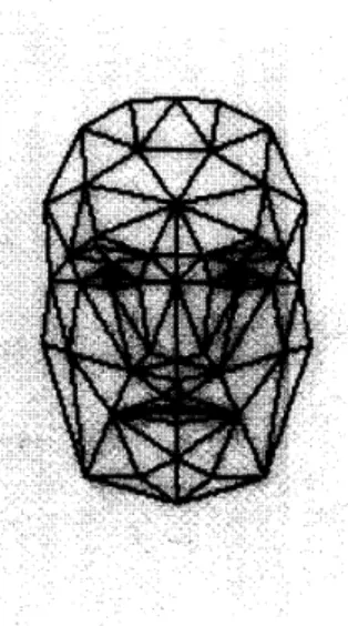
Fig. 1. Typical wireframe model made up of 100 triangles.

I

0.02

I

0.019933 0.020067 0.019939 0.05

I

0.05004 0.049967 0.050031

2) Determine the motion parameters from (5) using the given depth values.

3) Compute

(XI'),

y!')), which are the coordinates of the match- ing points that are predicted by the present estimates of the motion and depth parameters (4). Compute the model prediction error (7) 1 .v En- = n; ,=O wx wy WZ where

True motion MBASIC Uniform Gaussian

0.01 0.07856 0.010241 0.010779

0.02 0.0 157 12 0.020504 0.02 1464 -0.01 -0.009994 -0.009996 -0.009984

e t = (si - x i k ) ) '

+

(y: - y!'))2. ₍₈₎

Here ( x : , y i ) are the actual coordinates of the matching points, which are given.

Else, set k = k

+

1, and perturb the depth parameters as 4) If El,

<

E, stop the iteration,

2:')+-

pl)

- ,?g(Z,)

+

a'& ( 9 ) where g ( Z ) is the gradient of e, with respect to 2, (which can be analytically computed from (4)) and cv and ,? are constants. For Gaussian distributed perturbations, At = N z ( O , a : ( k ) ) , i.e., zero mean Gaussian with variance

OB'

, where c$') = e,. For uniformly distributed perturbations, A t = UZ(Z!'-') f

0.5), i.e., uniformly distributed in an interval of length 1 about @ - ' ) , where U , denotes uniformly distributed random numbers. Since the range of the depth parameters are scaled to the interval (0, I), we truncate the value of the perturbed estimate to within this interval if the perturbation extends beyond the interval.

k )

5) Go to step (2).

The difference in computational complexity between the two al- gorithms originates from the estimation of the depth ( 2 ) parameters. The MBASIC algorithm treats this as another least squares estimation problem which requires seven multiplies and eight adds per point pair per iteration. Our method is based on perturbation of the depth parameters and requires 16 multiplies and 12 adds per point pair per iteration. Experimental results presented in the next section show that the MBASIC algorithm usually converges to a result in about

Tz

Tu

TABLE I

TRUE AND ESTIMATED MOTION PARAMETERS FOR 1o-POlNT CORRESPONDENCES WITH (a) lo%, (b) 30%, AND (c) 50% INVIAL ERROR IN THE D E ~ H ESTIMATES

I

0.02

11

0.018079 0.019966

I

0.021038

I

0.05

11

0.050961 0.050018

I

0.049481

11

True motion

I]

MBASIC

1

Uniform

I

Gaussian

w,

II

0.01

11

0.009951

I

0.010181

I

0.010141 w,

I[

0.02

11

0.0199901

I

0.020351

I

0.020255 w.

II

-0.01

11

-0.009994 1-0.009998 1-0.009995

Ty

11

0.05

11

0.052281

I

0.049818

I

0.050018

(4

5-1 0 iterations. Our algorithm generally provides superior results after about 15-20 iterations (see Figs. 2 4 ) . Considering that we work with 5-10 point pairs, the computational complexity of the improved algorithm is just slightly higher.

IV. RESULTS

In this section, we compare the performance of the proposed im- proved algorithm with that of the MBASIC algorithm in the presence of various degrees of inaccuracy in the initial depth estimates as well as for different numbers of point correspondences. The comparative analysis has been performed by means of a number of numerical simulations as well as an experiment with a typical videophone scene known as Claire. The wireframe model (CANDIDE) [ I ] consisting of 100 triangles as shown in Fig. 1 was used in the experiment with the Claire sequence.

The simulations were carried out by using five, seven, and 10 point correspondences, respectively, with 10, 30, and 50% error in the initial depth estimates in each case. The data for the simulations were generated as follows: A set of 5 to 10 points (zt, yz) with the respective depth parameters 2, in the range 0 and 1 were arbitrarily chosen. The coordinates (z:, y i ) of the matching points in the next frame were generated from ( x ~ , yt ) using the transformation (3) with the "true" 3-D motion parameters listed in Table I. Then, f 1 0 , f30, or f 5 0 % error is added to each depth parameter 2, for the respective simulations. The signs of the error (+ or -) were chosen randomly. At each iteration of the algorithm, first the motion parameters are estimated as the least squares solution (5) using the present depth parameters. (This step is the same as in the MBASIC algorithm.) Then, the depth parameters are updated as given by (9). We set cv = 0.95 and 3 ,! = 0.3 to obtain the reported results. We iterate

714

1

IEEE TRANSACTIONS ON IMAGE PROCESSING, VOL. 3, NO. 5, SEPTEMBER 1994

0.10 0.08 0.06 0 w 0.04 0.02 ___ Aizowa . . . Uniform Gaussian 0.00 0.0 20.0 40 a sa a 80.0 100 a Iteration number (a) 000 I 0.0 20.0 40.0 60.0 80 a 100.0 Itemtion number (a) 0.10 I 0.00 1 I 0 0 20.0 40.0 60.0 80.0 100.0 Itemtion number (h) 0.10

,

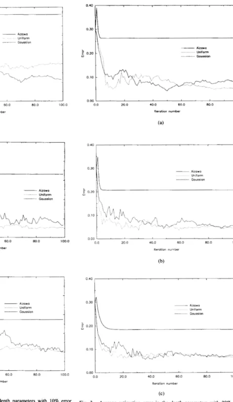
I 1 0.0 20.0 40.0 60 0 ea o i 00.0 ltetotion number

Fig. 2. Average estimation error in the depth parameters with 10% error in the initial depth estimates for (a) five-, (b) seven-, and (c) 10-point correspondences.

between (5) and (9) until E, given by (7) is less than an acceptable level. In order to minimize the effect of random choices in the evaluation of the results, the results are repeated three times using

o 4a 0 0 0 1 1 a a 20 a 40.0 60.0 8a a 1ao.a Iteration number 0.40 I a 0 0 1 I a a 20 0 40 a 60 0 80 0 iaa o Iteration number (C)

Fig. 3. Average estimation error in the depth parameters with 30% error in the initial depth estimates for (a) five-, (b) seven-, and (c) IO-point correspondences.

three different seed values for the random number generator. The results shown in Table I and Figs. 2 4 are the average of these three sets.

IEEE TRANSACTIONS ON IMAGE PROCESSING, VOL. 3, NO. 5, SEPTEMBER 1994 0.50 I 715 I 1.0

,

I

1

0.6

1

0.0 I I 0.0 20 0 40.0 60.0 80 0 100 Iteration number 0.60 I Uniform Govssian ... 0.00 0.0 20.0 40.0 60 0 80 0 100 0 Iteration number (b)

h

0.40 0.00 0.0 20 0 40 0 60.0 80 0 100.0 Iteratton number (c)

Fig. 4. Average estimation error in the depth parameters with SO% err01 in the initial depth estimates for (a) five-, (b) seven-, and (c) IO-point correspondences.

Table I provides a comparison of the motion parameter estimates obtained by the MBASIC algorithm and the proposed method using uniform and Gaussian distributed random perturbations at the conclu- sion of the iterations (in this case after 100 iterations). Table I shows

(b)

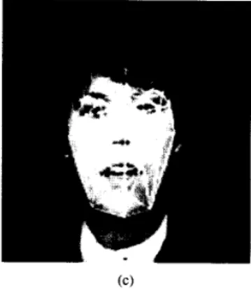
Fig. 5 . Wire-frame model fitting for a typical video-phone sequence Claire: (a) Wire-frame model fitted to the first frame; (b) modified wire-frame model for the seventh frame using the depth and motion parameters estimated by Aizawa's algorithm.

(C)

Fig. S. Wire-frame model fitting for a typical video-phone sequence Claire:

( c ) modified wire-frame model for the seventh frame using the proposed algorithm with uniform perturbations.

the results only for the 10-point correspondence case. The five- and seven-point results are similar. The comparison of the results of the depth parameter estimation is shown in Figs. 2 4 . In these figures, the average estimation error in the depth parameters versus iteration number is plotted, where the average error is defined as

where AV is the number of point correspondences and Z, and 2,

716 IEEE TRANSACTIONS ON IMAGE PROCESSING, VOL. 3, NO. 5. SEWEMBER 1994

are the “true” and estimated depth parameters, respectively. Note that the scale of the vertical axis is not the same in each case. Fig. 2(a)-(c) shows the estimation error when 10% error is present in the initial depth estimates for five, seven, and 10-point correspondences, respectively. Figs. 3(a)-(c) and 4(a)-(c) are for 30 and 50% error, respectively. In all these graphs, the solid line corresponds to the MBASIC algorithm and the dotted and the dashed lines correspond to the proposed algorithm with uniform and Gaussian perturbations, respectively.

In the MBASIC algorithm, the errors in the depth estimation directly affect the accuracy of the motion estimation and vice versa since the algorithm iterates between (5) and (6). This can be seen from Table I, where the error in the initial depth estimates mainly affects the accuracy of d J and d g , which are directly multiplied by

2 in both equations. Thus, in the MBASIC algorithm, the error in

d 2 and d v estimates increases as we increase the error in the initial

depth estimates (see Table I). Further, in the MBASIC algorithm, the error in the depth estimates (at convergence) increases with increasing error in the initial depth parameters (see, e.g., Figs. 2(c), 3(c), and 4(c)). In the proposed algorithm, however, because it uses (for depth estimation) an update scheme given by (9), which is indirectly tied to the current estimates of the motion parameter estimates, a smaller average error is obtained for depth parameter estimation (compared with the MBASIC algorithm) in all cases. As can be seen from Figs. 2 4 , the depth estimates, using the proposed method, converge closer to the correct parameters even in the case of 50% error in the initial depth estimates. For example, in the case of estimation using 10- point correspondences with 50% error in the initial depth estimates, the proposed method results in about 50% error after 100 iterations, whereas the MBASIC algorithm results in 35% error. In the 10% initial error case, the error at the end of the iterations is 5.5% in MBASIC algorithm and 2% in our algorithm. This improvement in the depth estimation of course results in better motion parameter estimation with the proposed method (see Table I).

The proposed method with uniform perturbations has also been applied to a typical videophone scene known as Claire. Here, seven- point pairs that are interactively specified are used. The coordinates of the corresponding points are determined using the block matching technique, where the block size is S x S and the search window is 10 x 10. Fig. 5(a) depicts the original wireframe model manually fitted to the first frame of the Claire sequence as in Aizawa et al. Fig. 5(b) and (c) shows the projection of the modified wireframe model onto

the image plane for the seventh frame using the estimated depth and motion parameters with the MBASIC and the proposed algorithms, respectively. Inspection of the results indicates a much better fit in the case of the proposed algorithm.

V. CONCLUSION

In this paper, we propose an improved algorithm for motion and structure estimation that uses point correspondences under ortho- graphic projection. The improvement is achieved by avoiding feeding the errors in the depth estimates back onto motion estimates. It is concluded that the proposed algorithm provides better results when the initial depth estimates contain significant random errors (which is the case in practice). A reasonably good performance has been demonstrated even in the presence of 50% error in the initial depth estimates. Computational complexity of the improved algorithm is just slightly higher.

REFERENCES

[ I ] R. Forchheimer and T. Kronander, “Image coding-from waveforms to animation,” IEEE Trans. Acoust. Speech Signal Processing, vol. 31, no. 12, pp. 2008-2023, Dec. 1989.

[2] W. J. Welsh, “Model-based coding of videophone images,” Electron.

Commun. Eng. J., pp. 29-36, Feb. 1991.

[3] K. Aizawa, C. S. Choi, H. Harashima, and T. S. Huang, “Human facial

motion analysis and synthesis with application to model-based coding,” in Morion Analysis and Image Sequence Processing, (M. 1. Sezan and R. L. Lagendijk, Eds.).

[4] K. Aizawa, H. Harashima, and T. Saito, “Model-based analysis-synthesis image coding (MBASIC) system for a person’s face,” Signal Processing:

Image Commun., no. I , pp. 139-152, 1989.

[5] Y. Nakaya, Y. C. Chuah, and H. Harashima, “Model-basedlwaveform hybrid coding for videophone images,” in Proc. Int. Conf ASSP’91, pp.

214 1-2144.

[6] M. Kaneko, A. Koike, and Y. Hatori, “Coding of facial image sequence based on a 3D model of the head and motion detection,” J. Visual Comm. Image Rep., vol. 2, no. 1, pp. 39-54, Mar. 1991.

[7] M. J. T. Reinders, B. Sankur, and J. C. A. van der Lubbe, “Transfor- mation of a general 3D facial model to an actual scene face,” in Proc.

11th Int. Con5 Part. Recog.,

[8] T. S. Huang and C. H. Lee, “Motion and structure from orthographic projections,” IEEE Trans. Pattern Anal. Machine Intell., vol. 11, no. 5, pp. 536540, May 1989.

[9] K. Zeger and A. Gersho, “Stochastic relaxation algorithm for improved vector quantizer design,” Electron. Left., vol. 25, no. 14, pp. 9 6 9 8 , July 1989.

Boston: Kluwer, 1993.