PREDICTING BUSINESS FAILURES IN
NON-FINANCIAL TURKISH COMPANIES
A Master’s Thesis
by
KAAN OKAY
Department of
Business Administration
İhsan Doğramacı Bilkent University
Ankara
September 2015
PREDICTING BUSINESS FAILURES IN
NON-FINANCIAL TURKISH COMPANIES
Graduate School of Economics and Social Sciences
of
İhsan Doğramacı Bilkent University
by
KAAN OKAY
In Partial Fulfilment of the Requirements for the Degree of
MASTER OF SCIENCE
in
THE DEPARTMENT OF BUSINESS ADMINISTRATION
İHSAN DOĞRAMACI BİLKENT UNIVERSITY
ANKARA
I certify that I have read this thesis and have found that it is fully adequate, in scope and in quality, as a thesis for the degree of Master of Science in Management.
Assist. Prof. Burcu Esmer Supervisor
I certify that I have read this thesis and have found that it is fully adequate, in scope and in quality, as a thesis for the degree of Master of Science in Management.
Assist. Prof. Ay¸se Ba¸sak Tanyeri Examining Committee Member
I certify that I have read this thesis and have found that it is fully adequate, in scope and in quality, as a thesis for the degree of Master of Science in Management.
Prof. Nuray G¨uner
Examining Committee Member
Approval of the Graduate School of Economics and Social Sciences:
Prof. Erdal Erel Director
ABSTRACT
PREDICTING BUSINESS FAILURES IN
NON-FINANCIAL TURKISH COMPANIES
Okay, Kaan
M.S., Department of Management Supervisor: Assist. Prof. Burcu Esmer
September, 2015
The prediction of corporate bankruptcies has been widely studied in the finance literature. This paper investigates business failures in non-financial Turkish companies between the years 2000 and 2015. I compare the accuracies of different
prediction models such as multivariate linear discriminant, quadratic discriminant, logit, probit, decision tree, neural networks and support vector machine
models. This study shows that accounting variables are powerful predictors of business failures one to two years prior to the bankruptcy. The results show that three financial ratios: working capital to total assets, net income to total assets, net income to total liabilities are significant in predicting business failures in non-financial Turkish companies. When the whole sample is used, all five models predict the business failures with at least 75% total accuracy, where the decision tree model has the best accuracy. When the hold-out samples are used, neural networks model has the best prediction power among all models used in this study.
Keywords: multivariate linear discriminant model, quadratic discriminant model, logit model, probit model, decision tree model, neural networks model, support vector machines, business failures, bankruptcy prediction, financial ratios .
ÖZET
FİNANSAL OLMAYAN TÜRK ŞİRKETLERİNDE
İFLAS TAHMİNİ
KAAN OKAY İşletme, Yüksek Lisans
Tez Yöneticisi: Yrd. Doç. Burcu Esmer Eylül, 2015
Kurumsal iflas tahmini finans literatüründe yaygın olarak incelenmistir. Bu tez 2000 ve 2015 yılları arasında finansal sektörde olmayan Türk şirketlerinin iflas tahminlerini 7 farklı modelin: çoklu değişkenli doğrusal diskriminant, ikinci derece diskriminant, logit, probit, karar ağacı, yapay sinir ağları ve destek
vektör makinesi modelleri doğruluklarını karşılaştırarak inceler. Bu çalışma, finansal oranlarn iflastan 1 ila 2 yıl öncesine kadar güçlü belirleyici olduklarını göstermektedir. Ayrıca, üç finansal oranın: döner sermayenin toplam aktiflere oranı, net gelirin toplam aktiflere oranı ve net gelirin toplam pasiflere oranının iflas tahminini öngörmede önemli olduğunu göstermektedir. Bütün veri seti kullanıldığında, karar ağacı modeli %75 ile en yüksek doğruluk oranına sahiptir. İkincil numuneler kullanıldığında ise yapay sinir ağları diğer modellere göre en yüksek doğruluk oranına sahiptir.
Anahtar sözcükler : çoklu değişkenli doğrusal diskriminant modeli, ikinci derece diskriminant modeli, logit modeli, probit modeli, karar ağacı modeli, yapay sinir ağları modeli, destek vektör makineleri, iflas tahmini, finansal oranlar .
Acknowledgement
Firstly, I would like to express my sincere gratitude to my supervisor Assist. Prof. Burcu Esmer for her continuous support, patience and motivation. Her guidance helped me in all the time of research and writing of this thesis.
Besides my supervisor, I would like to thank the rest of my thesis committee:
Assist. Prof. Ay¸se Ba¸sak Tanyeri, Assist. Prof. Mirza Troki´c for their insightful
comments.
Last but not the least, I would like to thank my family: my parents and to my brother for supporting me throughout writing this thesis.
Contents
1 Introduction 1
2 Literature Review 5
3 Models 11
3.1 Multivariate Discriminant Analysis . . . 11
3.2 Quadratic Discriminant Analysis . . . 13
3.3 Logit Model . . . 13
3.4 Probit Model . . . 14
3.5 Decision Tree . . . 15
3.6 Neural Networks . . . 16
3.7 Support Vector Machine . . . 17
4 Data 19 5 Results 25 5.1 Results of Multivariate Discriminant Analysis . . . 25
CONTENTS vii
5.2 Results of Quadratic Discriminant Analysis . . . 26
5.3 Results of Logit Model . . . 27
5.4 Results of Probit Model . . . 27
5.5 Results of Decision Tree . . . 28
5.6 Comparison of Accuracy Levels Using Whole Sample . . . 30
5.7 Comparison of Accuracy Levels Using Holdout Samples . . . 30
List of Figures
3.1 Decision tree example . . . 15
3.2 Decision tree classification . . . 16
3.3 Neural networks model . . . 17
3.4 SVM model . . . 18
List of Tables
4.1 Delisting frequency . . . 20
4.2 Financial ratios . . . 22
4.3 Correlation matrix of variables . . . 23
4.4 Descriptive Statistics . . . 24
5.1 Type I and Type II errors for MDA . . . 26
5.2 Type I and Type II errors for QDA . . . 26
5.3 Logit Model . . . 27
5.4 Type I and Type II errors for LOGIT . . . 27
5.5 Probit Model . . . 28
5.6 Type I and Type II errors for PROBIT . . . 28
5.7 Type I and Type II errors for Decision Tree . . . 29
5.8 Comparison of Total Accuracy Rates . . . 30
Chapter 1
Introduction
With ever-growing business environment, accomplishment of a successful growth has become challenging. As a result, a lot of companies face financial strug-gles which lead them eventually to fail, affecting all stakeholders: employees, stockholders, managers, investors, and regulators. Bankruptcy prediction has at-tracted the attention of both academics and practitioners since the seminal works of Beaver (1966) and Altman (1968) in the late 1960s.
Especially in developing countries such as Turkey, the competition between companies is getting tougher with increasing number of listed companies each year. As of July 2015 there are over 500 companies in Borsa Istanbul (BIST). Government institutions agreed on a public offering campaign, in 2008, which aims to increase the number of listed companies in BIST up to one thousand by the year 2023. Thus, predicting business failures has become an important task to guide investors and regulators.
The aim of this study is to investigate business failures in non-financial Turk-ish companies between the years 2000 and 2015 and compare the accuracies of different prediction models. As Altman states, business failure is an ambiguous term. Karels and Prakash (1987) state there are many different definitions of bankruptcy used in literature, such as negative net worth, non-payment of cred-itors, bond defaults, inability to pay debts, over-drawn bank accounts, omission
of preferred dividends, receivership, inability of a firm to pay its financial obliga-tions as they mature etc. In this thesis, I follow Altman (2010) and use business failure as being delisted from the stock market. Generally, studies conducted in developed countries use the legal definition of bankruptcy, meaning filing a formal petition. However, since it may not be possible to reach complete financial ratios of failed companies, I assume bankruptcy as being delisted from stock market throughout the rest of our study.
In this study I use 32 failed and 32 non-failed non-financial Turkish companies to predict business failures between the years 2000 and 2015. I compare the accuracies of different prediction models such as multivariate linear discriminant, quadratic discriminant, logit, probit, decision tree, neural networks and support vector machine models. This study shows that accounting variables are powerful predictors of business failures one to two years prior to the bankruptcy. The results show that three financial ratios: working capital to total assets, net income to total assets, net income to total liabilities are significant in predicting business failures in non-financial Turkish companies. When the whole sample is used, all five models predict the business failures with at least 75total accuracy, where the decision tree model has the best accuracy. When the hold-out samples are used, neural networks model has the best prediction power among all models used in this study.
The prediction of bankruptcy has been studied by academics for a long time. Beaver, in his 1966 study, introduced the univariate approach of discriminant analysis for bankruptcy prediction. Altman (1968) adds to the univariate proach of Beaver (1966) and introduces the first multivariate discriminant ap-proach (MDA). Altman, Haldeman and Narayanan (1977) introduce the Zeta model where they use discriminant analysis (QDA) with log-transformations of variables to relax the assumptions of univariate analysis.
Until the 1980s, discriminant analysis has been widely used in the literature to predict business failures. In early 1980s, probabilistic statistical methods have been introduced. Ohlson (1980) is the first to use the conditional logit analysis on a large sample for the prediction of corporate bankruptcy to overcome the
statistical violations of discriminant analyses such as linearity, normality and independence among predictor variables.
Since 1990s, with the wide availability of computers, artificially intelligent methods such as neural networks (NN), support vector machine (SVM) and de-cision tree (DT) models have become more common in literature. Odom and Sharda (1990) show that accuracy rate for neural networks model is better com-pared to MDA. Min and Lee (2005) apply SVM to the bankruptcy prediction problem. They compare the performance of SVM with MDA, logit, and NN and conclude that SVM outperforms other models. Joos et al. (1998) conclude that decision tree model is superior to logit model when short term data is used.
Most studies which analyze bankruptcy using Turkish data focus on bankruptcy of banks during the early 2000s. Boyacioglu, Kara and Baykan (2009) use NN, SVM, and MDA predict bank failures in a sample of 21 failed and 44 non-failed banks between the years 1997- 2003. They conclude NN models per-form better than other models. Canbas, Cabuk and Kilic (2005) propose an integrated early warning system for privately owned banks by combining MDA, logit, probit and principal component analysis using a sample of 21 failed and 19 non-failed banks over the years 1996-2003. Erdogan (2008) employs logit analysis to predict bank failures using data between 1997 and 1999 period and validated using 1999-2001 data for prediction.
This study is closest to Ugurlu and Aksoy (2006) and Aktan (2011). Ugurlu and Aksoy (2006) employ MDA and logit models to predict financial distress in manufacturing companies. They use a sample of matched 27 failed and 27 non-failed companies over the years 1996 and 2003 and show that the logit model has the highest classification power and prediction accuracy. Aktan (2011) employs statistical, market based and machine learning approaches to develop cost sensi-tive prediction models. His data includes 180 industrial companies over the years 1997 and 1999 to predict bankruptcies in 2000.
This study adds to the bankruptcy prediction literature by focusing on a developing country and is the first to thoroughly investigate business failures for non-financial Turkish companies over a long period of time.
Outline of the rest of the thesis is as follows: Chapter 2 provides a detailed review of previous studies regarding bankruptcy prediction. In Chapter 3, models used in this thesis are explained in detail. Chapter 4 contains data selection process, where it is taken from, variable selection, matching and data descriptions. Chapter 5 consists of the results and their interpretations. Lastly, I conclude with Chapter 6.
Chapter 2
Literature Review
The prediction of bankruptcy has been studied by academics for a long time. One of the early attempt to predict bankruptcy is Fitzpatrick (1932). He uses the data of 20 matched sample of companies that bankrupt during the period 1920-1929 and he compares their accounting ratios such as current ratio, quick ratio and net worth to fixed assets without employing a statistical method to predict bankruptcy and concludes that the bankrupt companies have poorer ratios.
In 1966, the modern bankruptcy prediction literature began by Beaver. This study is the most widely accepted univariate study since it is a landmark for future research in ratio analysis. He uses a matched sample of 79 failed and 79 non-failed US companies to employ univariate discriminant analysis. This model considers the accounting ratios individually and a cut off point is calculated for each ratio to minimize misclassification costs. In his study, he finds that the cash flow to total debt ratio is the best predictor of bankruptcy for his sample. Other significant ratios are total debt to total assets and net income to total assets. His prediction accuracy ranges from 50% to above 90%.
In spite of its good predictions, the univariate discriminant analysis is later criticized. Univariate models may produce conflicting results for the same pany with different ratios.(Altman (1968)) Also, the financial situation of a com-pany does not depend on one factor. The univariate approach might not be
sufficient to capture all the aspects of failure. (Edmister (1972))
In 1968, Altman improves the univariate approach of Beaver (1966) and in-troduces the first multivariate discriminant approach (MDA). This is the well known Altman Z-score which is still widely used in academia and the industry as a benchmark model to compare accuracies of different models.
The main advantage of MDA over univariate approach is that it considers all variables common to the relevant company as well as their interactions with each other. Altman uses a matched sample of 33 failed and 33 non-failed US manufacturing companies between the years 1946 and 1965 and constructs a model with five accounting variables. The variables in the model are chosen based on their statistical significance, inter correlations, popularity in the literature and their potential relevancy. The predictive accuracy of the model is 95%, 72%, 48%, 29%, 36% accuracy for one, two, three, four and five years prior to bankruptcy, respectively and 79% for hold-out sample.
Following Altman’s multivariate discriminant methodology, many variations are derived and this methodology has become the most popular and frequently used model in literature and financial sector. New studies try to improve this model by changing variables, expanding the sample size, changing company types or adding quadratic terms.
In 1977, Altman, Haldeman and Narayanan (1977) introduce the Zeta model with seven variables. They use log-transformations of variables to improve their normality and quadratic discriminant analysis (QDA) to overcome the assump-tion of equal condiassump-tional covariance matrices which is required by the original Z-score model. The sample consists of 111 manufacturing and retailing compa-nies between the years 1969 and 1975. The bankrupt compacompa-nies are matched to healthy companies according to their industry and year of data. They find that the Zeta model outperforms alternative methods however, improving the statis-tical quality of the model does not necessarily improve the prediction accuracy of the model. Classification accuracy of this model is 96% prior to bankruptcy and 70% for five years prior to bankruptcy. Dillon and Goldstein (1984), Sanchez and Sarabia (1995) and Sharma (1996) use QDA and claim that MDA is a more
robust and accurate model compared to QDA when the independent variables are deviated from normality assumption.
In spite of the discriminant model’s good prediction accuracy, they are crit-icized by academics. This methodology provides a dichotomous classification of the companies and does not estimate the associated risk of bankruptcy. Moreover, the use of the model is restricted by statistical assumptions such as the linearity, normality and independence among predictor variables. These assumptions are usually violated in applications. Altman, Haldeman and Narayanan (1977) and Hamer (1983) show that improving the statistical quality of the model does not necessarily improve the prediction accuracy of the model.
The next improvement in bankruptcy prediction literature is the introduction of probabilistic statistical methods which are able to provide a probability of bankruptcy for each company. In 1980, Ohlson uses the conditional logit analysis on a large sample for the prediction of corporate bankruptcy to overcome the statistical violations of MDA. In contrast to the difficult interpretation of the Z-scores, conditional logit analysis results can be interpreted as the conditional probability of bankruptcy under less restrictive assumptions. Using a cut off point, which is calculated to minimize the costs of misclassification, a company is classified as bankrupt or non-bankrupt. Ohlson (1980) uses a large sample con-sisting of 105 bankrupt and 2000 non-bankrupt US industrial companies between the years 1970 and 1976 that did not involve pair matching. The accuracy of the model is 96%, 95% and 92% for prediction at bankruptcy within one year, two years and one or two years respectively.
Zmijewski (1984) uses different independent variables and studies adjustments of estimation bias resulting from oversampling for bankruptcy prediction models with non-random samples using probit models. Actually, probit model is very similar to logit model. The only difference is the link function in which probit uses a normal cumulative function instead of a logistic function.
Since 1990s, with the wide availability of computers, artificially intelligent methods such as neural networks, support vector machine and decision tree mod-els have become more common in literature. Among these techniques, neural
networks (NN) model is the most widely used. NN is inspired by biological neu-ral networks of the human nervous system. They learn from training examples using different algorithms just like a human being learns. The structure of the model takes form according to information from the training data and generally uses non-linear equations to estimate outputs that depends on many inputs. NN does not suffer from statistical assumptions as traditional statistical models.
Odom and Sharda (1990) is the first to use NN for prediction of bankruptcy. They use the same financial variables used in Altman’s Z-score. Their sample consist of 65 bankrupt and 64 non-bankrupt companies between 1975 and 1982, overall 129 companies. Among these 129 companies, they use 74 of them to train their model and remaining 55 companies to test their model. They also employ MDA as benchmark model. They conclude that the accuracy rate of NN is 82% for holdout sample while MDA’s accuracy rate is 74%.
Zhang et al. (1999) compare NN’s performance with logit model using a sample of manufacturing companies. The NN significantly outperforms the logit regression model with accuracy of 80% versus 78% for small test set and with accuracy of 86% versus 78% for large test set.
Fletcher and Goss (1993) compare a NN with a logit model using a sample of 36 bankrupt and non-bankrupt companies. Their model consists of three financial ratios which are current ratio, quick ratio and working capital to net income. They conclude that NN has higher accuracy rate compare to logit model at almost all cutoff points. The other significant contributors that use NN are Boritz, Kennedy and Albuquerque (1995), Charitou, Neophytou and Charalambous (2004), Coats and Fant (1993)
Another machine learning model is support vector machine (SVM). The liter-ature on this model is relatively narrow compared to NN or traditional statistical models. It is a comparatively new model and has certain advantages on small samples. SVM is a blend of linear discriminant function and instance based learn-ing algorithm, that selects a number of critical boundary points which are called support vectors. Basically, SVM uses a linear function to classify observations by mapping non-linear input vectors into a higher dimensional feature space. Shin,
Lee, and Kim (2005) use SVM and compare the results with NN model. They show that the generalization performance of SVM is better than NN as the sam-ple size gets smaller. Min and Lee (2005) compare the performance of SVM with MDA, logit, and NN and conclude that SVM outperforms other models.
Another model used in bankruptcy prediction is decision tree model. This model uses recursive partitioning technique to split the observations into subsets. The process continues until recursive partitioning no longer adds value to pre-dictions. Decision tree models have certain advantages over classical statistical models. They are not affected from statistical restrictions such as non-linearity and non-normality. They are simple and provide an intuitive insight.
Joos et al. (1998) compare decision tree and logit models in a credit classifi-cation environment. They use an extensive database of one of the largest Belgian banks and find that logit model outperforms decision tree model in terms of cost efficiency and for a qualitative data set, decision tree model is superior to logit model. The other significant contributors that use decision tree model are Henly and Hand (1996), Zheng and Yanhui (2007)
In Turkey, there are a few studies that attempt to predict bankruptcy. Most of them focus on bankruptcy of financial companies during the early 2000s. Boy-acioglu, Kara and Baykan (2009) uses neural networks, support vector machines and multivariate statistical methods to predict bank failures in a sample of 21 failed and 44 non-failed banks between the years 1997-2003. They conclude that all models perform well and neural network models performs better than other models.
Canbas, Cabuk and Kilic (2005) propose an integrated early warning system for privately owned banks by combining MDA, logit, probit and principal com-ponent analysis using a sample of 21 failed an 19 non-failed banks over the years 1996-2003. They conclude that banks can avoid restructuring costs in the long run if they use this integrated early warning system.
Erdogan (2008) employs logit analysis to predict bank failures in 1999-2001 by using the data between 1997 and 1999. They argue that 80% of failed banks
could be predicted two years before and logistic regression can be used as a part of an early warning system.
Ugurlu and Aksoy (2006) employ MDA and logit models to predict financial distress in manufacturing companies. They use a sample of matched 27 failed and 27 non-failed companies over the years 1996 and 2003. They find that the logit model has higher classification power and prediction accuracy.
Aktan (2011) employs statistical, market based and machine learning ap-proaches to develop cost sensitive prediction models. He uses data from a sample of 180 industrial companies over the years 1997 and 1999 to predict bankruptcies in 2000. He finds that all models have 90% or more classification accuracy one year prior to bankruptcy except discriminant, decision tree and KMV-Merton model. The discriminant analysis has the lowest accuracy rate with 76%.
The bankruptcy prediction literature has long history. Despite the numerous studies, there seems to be a lack of consensus as to which methodology is the most reliable. Also, the majority of the studies focus on developed countries. So, further investigation of the performance of prediction models is necessary in order to find the most suitable model for non-financial Turkish companies.
Chapter 3
Models
In this chapter, we explain the models in detail, including their assumptions and how they are incorporated into our study.
I will begin with traditional statistical models. The first model from this group is the multivariate linear analysis which is the most frequently used model in bankruptcy literature. Second, I will introduce the quadratic discriminant analysis which has less strict assumptions. The next models from traditional statistical models will be the logit and probit models. These two models represent the probabilistic approach.
Next, I will introduce the machine learning models which are decision tree, neural networks and support vector machine models. These models are com-paratively new and they have promising results in applications. They employ different algorithms to make data driven classifications and they are not affected from statistical assumptions as much as statistical models.
3.1
Multivariate Discriminant Analysis
The purpose of the multivariate linear discriminant analysis (MDA) is to find a linear combination of predictors to maximize the variance between failed and
non failed companies while minimizing the variance within failed (non-failed) companies. It is originally used for classification problems where the dependent variable is in qualitative form. In the bankruptcy prediction framework, this is equivalent to testing the hypothesis of a firm’s bankruptcy within the nearest year against the alternative of it not becoming bankrupt in the foreseeable future (Altman(1968)).
The MDA has the advantage of considering an entire profile of characteristics common to the relevant company, as well as the interaction of these characteris-tics. The basic form of the model is shown in equation (3.1).
Z = β0+ β1X1j + β2X2j+ ... + βnXnj, (3.1)
βi(i = 1, 2, ..., n) = coef f icient (discriminant) weights.
Xi(i = 1, 2, ..., n) = independent variables(i.e., the f inancial ratios.)
This one dimensional equation transforms individual financial ratios to a sin-gle discriminant score or Z value for every sinsin-gle company. A cut off point which calculated to minimize misclassification costs is compared to Z score of a com-pany for reclassification. If this Z score is greater than cut off number, then the company is classified as non-distressed. If Z score is less than the cut off point, then the company is classified as distressed.
The use of the model is restricted by two strong statistical assumptions. First, the multivariate normality of independent variables within each group and second, the equal variance-covariance matrices of two groups. These assumptions are often violated in applications.
3.2
Quadratic Discriminant Analysis
The purpose of the quadratic discriminant analysis (QDA) is to find a quadratic combination of predictors to maximize the variance between failed and non failed
companies while minimizing the variance within failed (non-failed) companies. The only difference between MDA and QDA is the latter allows each group distribution to have its own variance-covariance matrices. In fact, QDA can be seen as a general version of MDA with less statistical assumptions.
However, using quadratic form does not necessarily improve classification ac-curacy as indicated by Hamer (1983) and Altman et al. (1977).
Dillon and Goldstein (1984), Sanchez and Sarabia (1995) and Sharma (1996) use QDA and claim that MDA is actually more robust and accurate compare to QDA when the normality assumption does not hold for the independent variables.
q(x) = XT −1 2 −1 X 1 − −1 X 2 !! X + −1 X 1 µ1− −1 X 2 µ2 !T X (3.2)
QDA model is shown in the equation (3.2). QDA assumes independent vari-ables to be jointly multivariate normal and two groups do not have the same variance-covariance matrices. If the variance-covariance matrices are the same, then the equation (3.2) reduces to MDA since the first term on the right hand side will be zero.
3.3
Logit Model
The purpose of the logistic regression is to predict a discrete outcome such as group membership from a set of variables that may be continuous, discrete,
dichotomous, or a mix. In the bankruptcy prediction framework, estimation
problem can be reduced simply to the following statement: given that a firm belongs to some pre-specified population, what is the probability that the firm fails within some pre-specified time period? Since no assumptions have to be made regarding prior probabilities of bankruptcy and the distribution of predic-tors (Ohlson(1980)), logit model avoids the problems MDA has.
P = 1
1 + eβTX, (3.3)
βi(i = 1, 2, ..., n) = coef f icient (discriminant) weights;
Xi(i = 1, 2, ..., n) = independent variables, the f inancial ratios.
Equation (3.3) shows that the logit function maps the value of βTX to a
probability, P. Therefore, it is bounded between 0 and 1.
Logistic regression answers the same questions as discriminant analysis. There are no assumptions about the distributions of the independent variables, there-fore, more flexible compare to linear discriminant analysis. The independent variables do not have to be normally distributed, have equal variance covariance matrices within each group, or linearly related to the dependent variable.
One of the major drawback of this model is the instability of the coefficients when there is complete or quasi-complete separation of the companies, resulting in insignificant coefficients.
3.4
Probit Model
The only difference between the logit model and the probit models is the link function, Probit model uses a normal cumulative function instead of a logistic function. All other interpretations are the same as the logit model.
P = Z βix −∞ 1 √ 2πe −t2/2 dt = φ(βix) (3.4)
The equation (3.4) shows the probit model. P is the probability of bankruptcy as in logit model. The main purpose of using probabilistic models instead of discriminant analysis is to achieve higher accuracy levels. Comparative studies have different claims regarding the performances of these models and there does not seem a consensus.
3.5
Decision Tree
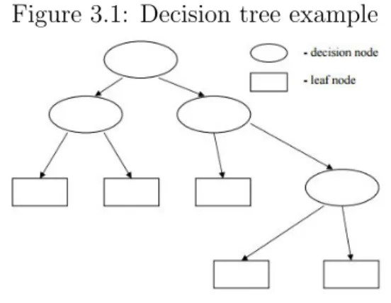
The majority of the tree models are used to solve classification problems. A decision tree compose of decision and leaf nodes as shown in Figure 3.1. Each decision node tests a particular characteristic of an observation.
Figure 3.1: Decision tree example
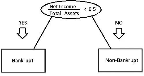
A very simple example on how the model classifies an observation is shown in Figure 3.2. The model determines the split for net income to total assets ratio is as 0.5. So, if a company has ratio lower then 0.5, it will be classified as bankrupt. If its ratio is higher then 0.5, it will be classified as non-bankrupt. Decision tree models can have complex decision rules to follow. The important questions are which explanatory variables should be used and at which value the split should occur.
The tree model follows these steps to determine the splits and explanatory variables; at the beginning, the whole sample is considered as a single class. The split minimizing the class differences is chosen by recursive partitioning and then the class is split into two subsets using a variable. The process continues until no longer additional value is added to predictions.
Decision tree models have certain advantages over classical statistical models. They are not affected from statistical restrictions such as linearity and non-normality. They are simple and provide an intuitive insight.
Figure 3.2: Decision tree classification
3.6
Neural Networks
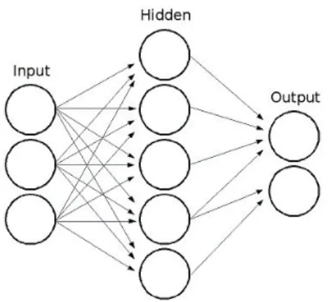
A neural networks model (NN) relates a set of input variables to output variables. The main difference from other approximation methods is that the NN model has hidden layers where the inputs are transformed by a special class of algorithms. This hidden layer approach is an efficient way to model non-linear statistical processes.
For representative purposes, there is an example in Figure 3.3. Three main part of the NN model is shown clearly, these are input layers which are indepen-dent variables, hidden layers that transform information flows from input layers and lastly the output layers where the desired solution is provided. This type of NNs are called multilayer perceptron. The information follows one way direction from input layers to hidden layers and then lastly to output layers.
Usual application of NN model in bankruptcy prediction literature is as fol-lows, the sample is arbitrarily divided into training and test samples. In the training sample, NN model learns the patterns and determines the linking weights of the nodes. In the test sample, model classifies new observations into groups based on training.
Figure 3.3: Neural networks model
3.7
Support Vector Machine
Support vector machine (SVM) is a blend of linear functions and instance based learning algorithms, that selects a number of critical boundary points which are called support vectors. Basically, SVM uses a linear function to classify observa-tions by mapping their non-linear input vectors into a higher dimensional feature space.
In this new space, an optimal separating hyper-plane is constructed and the observations that are closest to the maximum hyper plane are called support
vectors. SVM classifies observations based on these support vectors. That0s why
the model works well with small samples. The observations that are not support vectors are irrelevant for classification.
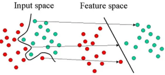
In Figure 3.4 depicts how SVM works. In the two dimensional input space, it is seen that the boundary that separates two groups is not linear. The first step is to find the separating feature space which maximizes the margin between
Figure 3.4: SVM model
the groups. When there is not a linear separator, SVM projects data points into a higher dimensional space where the groups become linearly separable. This is done via kernel trick.
The usual application of SVM is similar to NN model. The sample is randomly divided into two sub-samples as test and training samples.
Chapter 4
Data
The bankruptcy data for this study consists of 32 delisted Turkish companies excluding financial institutions and acquired companies. These companies were delisted due to following reasons from The Borsa Istanbul markets permanently between years 2000 and 2015:
• Filing for bankruptcy • Being financially distressed • Loss in consecutive 3 years • 2/3 asset value loss
• Negative equity figure
We have only considered companies for which financial data was available on Bloomberg. The ticker name of the delisted companies were obtained from
www.borsaistanbul.com. 1
1The total number of delistings is 97. Out of 97 delisted companies, 25 of them are acquired,
I match each failed company with a non-failed company based on closest total
asset size and year2 3 . I use the data of at least 1 year prior to delisting to ensure
that the data exist before the company delisted. For 17 out of 32 company, I use
the data of 2 year prior to bankruptcy due to lack of data. 4
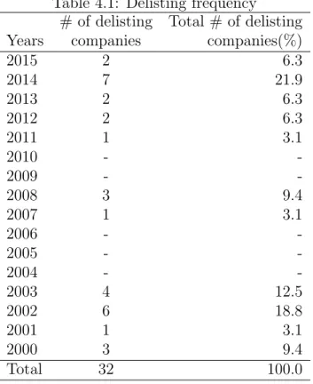
The frequency of delistings is displayed in Table 4.1. Table 4.1: Delisting frequency
# of delisting Total # of delisting
Years companies companies(%)
2015 2 6.3 2014 7 21.9 2013 2 6.3 2012 2 6.3 2011 1 3.1 2010 - -2009 - -2008 3 9.4 2007 1 3.1 2006 - -2005 - -2004 - -2003 4 12.5 2002 6 18.8 2001 1 3.1 2000 3 9.4 Total 32 100.0
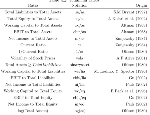
The variables are selected based on the existing literature and availability. However, different studies show different ratios as significant. So, I have collected the most frequently used variables in literature to the extent of availability on Bloomberg. The list of the all ratios is shown in Table 4.2.
2I call the delisted companies as failed companies.
3When I match a failed company with a non-failed company based on industry, asset size of
some pairs might become different. Therefore, I match based on only asset size.
4This situation actually works against the models since the effects of the financial distress
The first step in my study is to select good predictive variables. Correlation analysis is the starting point since almost all financial ratios exhibit some de-gree of correlation between each other. Table 4.3 shows the correlation matrix of explanatory variables. It can be seen that most of the ratios exhibit high cor-relation between each other and some ratios are transformations of each other. If correlation coefficient is higher than 0.5 between two variables, I prioritize the most frequently used and best performing variable.
The second step is looking at the statistical significance of the ratios. I use Akaike Information Criterion (AIC) in a stepwise algorithm to reach the final choice of the variables. AIC is known in the statistics as a penalized log-likelihood.
AIC = −2 x log − likelihood +2(p + 1)
Where p is the number of parameters in the model, and 1 is added for the estimated variance.
It is possible to obtain a perfect fit if we had separate parameter for every individual company, but this model does not have any explanatory power. There is always a trade off between the goodness of fit and the number of variables in the model. AIC is useful because it penalizes any unnecessary variables in the model, by adding 2(p + 1) to the deviance. When comparing different models, the lower the AIC is, the better the fit is.
Table 4.2: Financial ratios
Ratio Notation Origin
Total Liabilities to Total Assets lia/as S.M Bryant (1997) Total Equity to Total Assets eq/as J. Kolari et al. (2002)
Working Capital to Total Assets wc/as Altman (1968)
EBIT to Total Assets ebit/as Altman (1968)
Net Income to Total Assets ni/as Zmijewsky (1984)
Current Ratio cr Zmijewsky (1984)
1/Current Ratio 1/cr Ohlson (1980)
Volatility of Stock Prices vola A.F Atiya (2001)
Total Assets ≥ T otalLiabilities binaryasset Ohlson (1980) Working Capital to Total Liabilities wc/lia M. Leshno, Y. Spector (1996)
EBIT to Total Liabilities ebit/lia Gu (2002)
Net Income to Total Liabilities ni/lia Park (2002)
Working Capital to Total Equity wc/eq B.Back et al. (1996)
EBIT to Total Equity ebit/eq Gu (2002)
Net Income to Total Equity ni/eq Park (2002)
T able 4.3: Correlation matrix of v ariables lia/as eq/as w c/as ebit/as ni/as cr 1/c r v ola binary asset w c/lia ebit/lia ni/lia w c/eq ebit/eq ni/eq log(as) lia/as 1 -1 -0 .966 -0 .195 -0 .425 -0 .148 0 .902 0 .215 -0 .674 -0 .139 -0 .172 -0 .193 0 .144 -0 .026 0 .022 -0 .329 eq/as -1 1 0 .966 0 .195 0 .425 0 .148 -0 .902 -0 .215 0 .674 0 .139 0 .172 0 .193 -0 .144 0 .026 -0 .022 0 .329 w c/as -0 .966 0 .966 1 0 .233 0 .362 0 .162 -0 .936 -0 .251 0 .619 0 .155 0 .185 0 .190 -0 .135 0 .027 -0 .004 0 .295 ebit/as -0 .195 0 .195 0 .233 1 0 .547 0 .062 -0 .157 -0 .137 0 .257 0 .049 0 .464 0 .282 0 .166 0 .336 0 .480 0 .354 ni/as -0 .425 0 .425 0 .362 0 .547 1 0 .150 -0 .202 -0 .589 0 .703 0 .137 0 .311 0 .450 -0 .039 0 .256 0 .157 0 .337 cr -0 .148 0 .148 0 .162 0 .062 0 .150 1 -0 .080 -0 .094 0 .154 0 .999 0 .807 0 .521 0 .113 0 .028 0 .006 -0 .214 1/cr 0 .902 -0 .902 -0 .936 -0 .157 -0 .202 -0 .080 1 0 .091 -0 .444 -0 .076 -0 .093 -0 .090 0 .127 -0 .003 -0 .001 -0 .276 v ola 0 .215 -0 .215 -0 .251 -0 .137 -0 .589 -0 .094 0 .091 1 -0 .371 -0 .088 -0 .103 -0 .140 0 .141 -0 .008 0 .100 -0 .192 binary asset -0 .674 0 .674 0 .619 0 .257 0 .703 0 .154 -0 .444 -0 .371 1 0 .143 0 .196 0 .261 -0 .434 0 .193 -0 .310 0 .242 w c/lia -0 .139 0 .139 0 .155 0 .049 0 .137 0 .999 -0 .076 -0 .088 0 .143 1 0 .793 0 .513 0 .107 0 .025 0 .004 -0 .226 ebit/lia -0 .172 0 .172 0 .185 0 .464 0 .311 0 .807 -0 .093 -0 .103 0 .196 0 .793 1 0 .461 0 .157 0 .175 0 .157 0 .044 ni/lia -0 .193 0 .193 0 .190 0 .282 0 .450 0 .521 -0 .090 -0 .140 0 .261 0 .513 0 .461 1 0 .120 0 .157 0 .161 0 .047 w c/eq 0 .144 -0 .144 -0 .135 0 .166 -0 .039 0 .113 0 .127 0 .141 -0 .434 0 .107 0 .157 0 .120 1 -0 .062 0 .614 -0 .081 ebit/eq -0 .026 0 .026 0 .027 0 .336 0 .256 0 .028 -0 .003 -0 .008 0 .193 0 .025 0 .175 0 .157 -0 .062 1 0 .281 0 .153 ni/eq 0 .022 -0 .022 -0 .004 0 .480 0 .157 0 .006 -0 .001 0 .100 -0 .310 0 .004 0 .157 0 .161 0 .614 0 .281 1 0 .159 log(as) -0 .329 0 .329 0 .295 0 .354 0 .337 -0 .214 -0 .276 -0 .192 0 .242 -0 .226 0 .044 0 .047 -0 .081 0 .153 0 .159 1
Following the selection procedure, working capital to total assets, net income to total assets and net income to total liabilities are chosen to be used in the models.
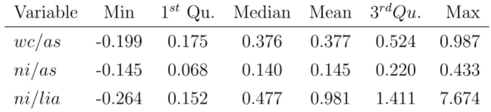
Table 4.4 shows the descriptive statistics for these variables for failed compa-nies and non-failed compacompa-nies. The means of all variables of failed group are less than the non-failed group as expected.
Table 4.4: Descriptive Statistics Failed Companies
Number of observations: 32
Variable Min 1st Qu. Median Mean 3rd Qu. Max
wc/as -14.079 -0.476 -0.121 -1.106 0.181 0.538
ni/as -1.962 -0.578 -0.106 -0.309 0.048 0.264
ni/lia -1.174 -0.340 -0.046 -0.168 0.081 0.447
Non-failed Companies Number of observations: 32
Variable Min 1st Qu. Median Mean 3rdQu. Max
wc/as -0.199 0.175 0.376 0.377 0.524 0.987
ni/as -0.145 0.068 0.140 0.145 0.220 0.433
Chapter 5
Results
In this chapter I show and compare the total accuracy ratios, type I and type II errors of the models.
• Total accuracy is the probability of correctly classifying a firm.
• Type I error is the probability of misclassifying a failed firm as non-failed. • Type II error is the probability of misclassifying a non-failed firm as failed
firm.
It is generally assumed that Type I error might be costlier then type II error. In case of type I error, investor or creditor may loss all principal and interest however, type II error can be seen as a missed opportunity rather then a loss.
5.1
Results of Multivariate Discriminant
Anal-ysis
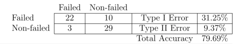
Z = 0.146wc as + 1.497 ni as + 0.508 ni liaTable 5.1: Type I and Type II errors for MDA
Failed Non-failed
Failed 22 10 Type I Error 31.25%
Non-failed 3 29 Type II Error 9.37%
Total Accuracy 79.69%
Above, the discriminant function with estimated coefficients are shown. In MDA model, a company is likely to fail as its Z score decreases. The signs of the coefficients are all positive as expected since the means of the failed group is less then the non-failed group.
In Table 5.1, total accuracy of the model is 79.69% which is quite impressive however type I error is higher compare to type II error.
5.2
Results of Quadratic Discriminant Analysis
Quadratic Discriminant Analysis (QDA)
Table 5.2: Type I and Type II errors for QDA
Failed Non-failed
Failed 19 13 Type I Error 40.63%
Non-failed 2 30 Type II Error 6.25%
Total Accuracy 76.55%
In Table 5.2, total accuracy of the QDA model is 76.55% which is comparable to MDA however most of the classification error is coming from the type I error which is assumed to be more costly than the type I error.
5.3
Results of Logit Model
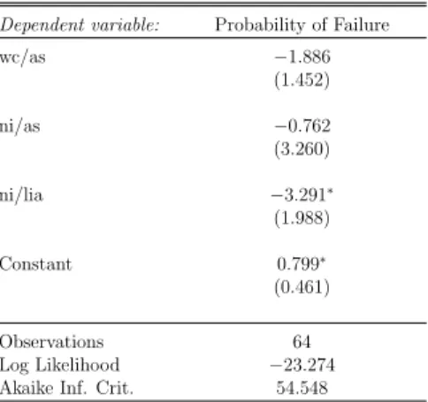
Estimated coefficients for the logit model are shown in Table 5.3. The terms inside the parenthesis are the standard errors. The signs of the coefficients are negative, indicating bankruptcy probability is increasing with lower values. Working capital to total assets and net income to total assets are not significant due to quasi
perfect separations of the group members. 1
Table 5.3: Logit Model Dependent variable: Probability of Failure
wc/as −1.886 (1.452) ni/as −0.762 (3.260) ni/lia −3.291∗ (1.988) Constant 0.799∗ (0.461) Observations 64 Log Likelihood −23.274
Akaike Inf. Crit. 54.548
Note: ∗p<0.1;∗∗p<0.05;∗∗∗p<0.01
Table 5.4: Type I and Type II errors for LOGIT
Failed Non-failed
Failed 25 7 Type I Error 21.88%
Non-failed 8 24 Type II Error 25%
Total Accuracy 76.56%
The total accuracy of the logit model is comparable to MDA and QDA.
5.4
Results of Probit Model
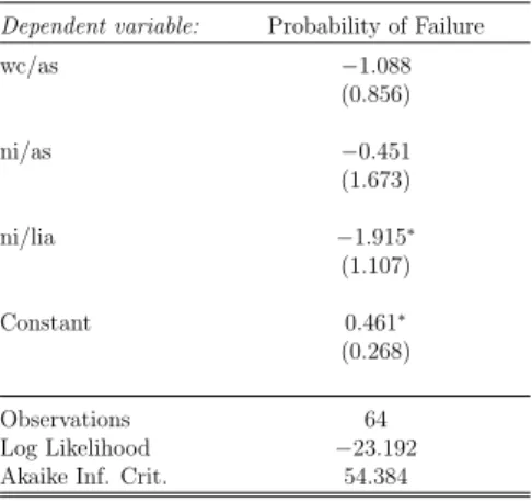
Table 5.5 shows the estimated coefficients for the probit model. The terms inside the parenthesis are the standard errors. The signs of the coefficients are negative, 1All variables are kept inside the model since omitting insignificant variables decreases the
indicating bankruptcy probability is increasing with lower values of independent variables. Working capital to total assets and net income to total assets are not significant as in logit model. Similar to logit regression, it is caused by quasi perfect separations of the group members.
Table 5.5: Probit Model Dependent variable: Probability of Failure
wc/as −1.088 (0.856) ni/as −0.451 (1.673) ni/lia −1.915∗ (1.107) Constant 0.461∗ (0.268) Observations 64 Log Likelihood −23.192
Akaike Inf. Crit. 54.384
Note: ∗p<0.1;∗∗p<0.05;∗∗∗p<0.01
Table 5.6: Type I and Type II errors for PROBIT
Failed Non-failed
Failed 26 6 Type I Error 18.75%
Non-failed 7 25 Type II Error 21.88%
Total Accuracy 79.69%
The total accuracy of the model is slightly better than the logit model. Also, the type I error is lower. For our sample, probit model has better prediction results.
5.5
Results of Decision Tree
Figure 5.1 shows the decision tree model. According to the splits detected by recursive partitioning,
• if working capital to total assets ratio of a company is less then 0.02, it is likely to bankrupt.
Figure 5.1: Decision tree model
• If working capital to total assets ratio is between 0.02 and 0.23 and net income to total assets ratio is less than 0.23, then it is likely to bankrupt.
All other observations that do not fit these rules are classified as non-bankrupt. Table 5.7: Type I and Type II errors for Decision Tree
Failed Non-failed
Failed 28 4 Type I Error 12.5%
Non-failed 3 29 Type II Error 9.37%
Total Accuracy 89.06%
The decision tree model has the highest accuracy among all other models with 89% accuracy rate. Moreover, it has the lowest type I error.
5.6
Comparison
of
Accuracy
Levels
Using
Whole Sample
Table 5.8 shows the summary of the accuracy results obtained by using the whole sample. When we compare these five models, decision tree model outperforms the others. MDA and the probit model have the same accuracy rate. However, type I error of MDA is 31% which is higher than type I error of probit model which is 18.8%.
Table 5.8: Comparison of Total Accuracy Rates
Models % of Correct Classifications % of Type I Error
1 − M DA 79.69 31.25
2 − QDA 76.55 40.63
3 − LOGIT 76.56 21.88
4 − P ROBIT 79.69 18.75
5 − T REE 89.06 12.5
Total number of observations = 64
5.7
Comparison of Accuracy Levels Using
Hold-out Samples
In this section, all 7 models are tested using hold-out samples. I randomly divide the sample into two sub-samples as training and test samples. I use training sample to estimate parameters and then I use the test sample to classify based
on models established. 2
With this procedure, I can use NN and SVM models which require test and training samples inherently and validate my results if there is a bias. When the companies that are used for coefficient estimation are reclassified, there is a possibility of upward bias. I use holdout samples to address this issue and compare 7 models simultaneously.
2Five replications of this procedure are created and tested. Based on these training examples,
Table 5.9 shows the average total accuracy rates of the models for holdout samples. The significance of the results are at 0.025 (*), 0.0025 (**) and 0.001 (***).
Table 5.9: Comparison of Test Samples Accuracy Rates
Models % of Correct Classifications Value of t
1 − M DA 77.5 3.1** 2 − QDA 79.4 3.3** 3 − LOGIT 76.9 3.0** 4 − P ROBIT 76.9 3.0** 5 − T REE 68.1 2.1* 6 − N N 81.3 3.5*** 7 − SV M 78.8 3.3**
Total number of observations per replication = 32
Tree model has the lowest accuracy with 68% accuracy rate. This is surprising since the tree model is the most accurate model when we use all sample. The reason for this result might be due to overfitting.
The traditional statistical models which are MDA, QDA, logit and probit, have similar results. NN model has the best predictive accuracy among all other models.
They are all significant indicating that the models have the discriminating power not only in the same sample but also in holdout samples. Therefore, the models are seem to be robust.
Chapter 6
Conclusion
Bankruptcy prediction models have been widely studied in the finance litera-ture. Various studies analyze different sample periods and different industries and compare the accuracy of different models to predict bankruptcy. In this study, I empirically test 7 widely used models to predict bankruptcy of listed Turkish non-financial companies using the data from 2000 to 2015.
I show that profitability and liquidity ratios such as net income to total assets, working capital to total assets, and net income to total liabilities are significant when predicting business failures.
When I use the whole sample, MDA, QDA, logit, probit and decision tree models predict failures with more than 76% accuracy rate. The decision tree model most accurately estimates business failures with 89% accuracy rate. Since there may be an upward bias when the whole sample is used. I randomly split the date into two sub-samples as training and test samples. I use the training sample to estimate parameters and then I use the test sample to predict failures. when this procedure is used, decision tree model performs the worst with 68% accuracy rate. This result confirms the overfitting of this model when the whole data is used. NN model performs the best among all seven models with 81% accuracy rate. This is due to the reason that NN model does not suffer from statistical assumptions as traditional statistical models.
Bibliography
S. Aktan. Application of machine learning algorithms for business failure predic-tion. Investment Management and Financial Innova, 2011.
E. I. Altman. Financial ratios, discriminant analysis and the prediction of corpo-rate bankruptcy. The journal of finance, 23:589–609, 1968.
E. I. Altman and E. Hotchkiss. Corporate financial distress and bankruptcy:
Predict and avoid bankruptcy, analyze and invest in distressed debt, volume 289. John Wiley & Sons, 2010.
E. I. Altman, R. G. Haldeman, and P. Narayanan. Zeta tm analysis a new model to identify bankruptcy risk of corporations. Journal of banking & finance, 1: 29–54, 1977.
E. I. Altman, G. Marco, and F. Varetto. Corporate distress diagnosis: Com-parisons using linear discriminant analysis and neural networks (the italian experience). Journal of banking & finance, 18:505–529, 1994.
W. H. Beaver. Financial ratios as predictors of failure. Journal of accounting research, pages 71–111, 1966.
J. E. Boritz and D. B. Kennedy. Effectiveness of neural network types for pre-diction of business failure. Expert Systems with Applications, 9:503–512, 1995.
M. A. Boyacioglu, Y. Kara, and ¨O. K. Baykan. Predicting bank financial failures
using neural networks, support vector machines and multivariate statistical methods: A comparative analysis in the sample of savings deposit insurance fund (sdif) transferred banks in turkey. Expert Systems with Applications, 36: 3355–3366, 2009.
S. Canbas, A. Cabuk, and S. B. Kilic. Prediction of commercial bank failure via multivariate statistical analysis of financial structures: The turkish case. European Journal of Operational Research, 166:528–546, 2005.
A. Charitou, E. Neophytou, and C. Charalambous. Predicting corporate failure: empirical evidence for the uk. European Accounting Review, 13:465–497, 2004. P. K. Coats and L. F. Fant. Recognizing financial distress patterns using a neural
network tool. Financial management, pages 142–155, 1993.
W. R. Dillon and M. Goldstein. Multivariate analysis: Methods and applications, volume 45. Wiley New York, 1984.
R. O. Edmister. An empirical test of financial ratio analysis for small business failure prediction. Journal of Financial and Quantitative analysis, 7:1477–1493, 1972.
B. E. Erdogan. Prediction of bankruptcy using support vector machines: an appli-cation to bank bankruptcy. Journal of Statistical Computation and Simulation, 83:1543–1555, 2013.
P. J. Fitzpatrick. A comparison of the ratios of successful industrial enterprises with those of failed companies. Accountants Publishing Company, 1932. D. Fletcher and E. Goss. Forecasting with neural networks: an application using
bankruptcy data. Information & Management, 24:159–167, 1993.
M. M. Hamer. Failure prediction: sensitivity of classification accuracy to alter-native statistical methods and variable sets. Journal of Accounting and Public Policy, 2:289–307, 1983.
W. Henley and D. J. Hand. A k-nearest-neighbour classifier for assessing consumer credit risk. The Statistician, pages 77–95, 1996.
P. Joos, K. Vanhoof, H. Ooghe, and N. Sierens. Credit classification: a comparison of logit models and decision trees. RUG, 1998.
G. V. Karels and A. J. Prakash. Multivariate normality and forecasting of business bankruptcy. Journal of Business Finance & Accounting, 14:573–593, 1987.
J. H. Min and Y.-C. Lee. Bankruptcy prediction using support vector machine with optimal choice of kernel function parameters. Expert systems with appli-cations, 28:603–614, 2005.
M. D. Odom and R. Sharda. A neural network model for bankruptcy prediction. In 1990 IJCNN International Joint Conference on neural networks, pages 163– 168, 1990.
J. A. Ohlson. Financial ratios and the probabilistic prediction of bankruptcy. Journal of accounting research, pages 109–131, 1980.
M. Sanchez and L. Sarabia. Efficiency of multi-layered feed-forward neural net-works on classification in relation to linear discriminant analysis, quadratic dis-criminant analysis and regularized disdis-criminant analysis. Chemometrics and Intelligent Laboratory Systems, 28:287–303, 1995.
S. Sharma. Applied multivariate techniques, 1996. USA, John Wiley& Sons. K.-S. Shin, T. S. Lee, and H.-j. Kim. An application of support vector machines
in bankruptcy prediction model. Expert Systems with Applications, 28:127–135, 2005.
M. Ugurlu and H. Aksoy. Prediction of corporate financial distress in an emerging market: the case of turkey. Cross Cultural Management: An International Journal, 13:277–295, 2006.
G. Zhang, M. Y. Hu, B. E. Patuwo, and D. C. Indro. Artificial neural networks in bankruptcy prediction: General framework and cross-validation analysis. European journal of operational research, 116:16–32, 1999.
Q. Zheng and J. Yanhui. Financial distress prediction based on decision tree models. In Service Operations and Logistics, and Informatics, 2007. SOLI 2007. IEEE International Conference on, pages 1–6. IEEE, 2007.
M. E. Zmijewski. Methodological issues related to the estimation of financial distress prediction models. Journal of Accounting research, pages 59–82, 1984.