NUMBERS IN POLITICS: COMPARATIVE
QUANTITATIVE ANALYSIS & MODELING IN
FOREIGN POLICY ORIENTATION AND ELECTION
FORECASTING
A Master ‘s Thesis
by
ENES TAYLAN
Department of
International Relations
İhsan Doğramacı Bilkent University
Ankara
NUMBERS IN POLITICS: COMPARATIVE QUANTITATIVE
ANALYSIS & MODELING IN FOREIGN POLICY ORIENTATION
AND ELECTION FORECASTING
Graduate School of Economics and Social Sciences of
İhsan Doğramacı Bilkent University by
ENES TAYLAN
In Partial Fulfillment of the Requirements for the Degree of MASTER OF ARTS
THE DEPARTMENT OF INTERNATIONAL RELATIONS
İHSAN DOĞRAMACI BILKENT UNIVERSITY ANKARA
ABSTRACT
NUMBERS IN POLITICS: COMPARATIVE QUANTITATIVE
ANALYSIS & MODELING IN FOREIGN POLICY ORIENTATION
AND ELECTION FORECASTING
Taylan, Enes
MA, Department of International Relations Supervisor: Assist. Prof. Dr. Özgür Özdamar
Co-Supervisor: Prof. Dr. Altay Güvenir May 2017
To advance social science in the direction of accurate and reliable quantitative models, especially in the fields of International Relations and Political Science, new novel methodologies borrowed from the Computer Science and Statistics should be employed. In International Relations, quantitative analysis can be carried out to understand foreign policy topic relations in public discourse of decision makers. In domestic politics, Election Forecasting is a suitable area, because of its offering of already quantified vote results and its importance in the decision-making process in domestic politics and foreign policy. This work embarks upon a
computational-
statistical model built on social media (Twitter) data and texts’ meaning extracted, analyzed and modeled with the state-of-the-art methodologies from Computer Science (Machine Learning and Natural Language Processing) and statistics to forecast
election results and foreign policy orientation. To verify the model, Turkish General Election 2015, US Presidential Election 2016 and campaign period of Donald Trump are analyzed. This work shows that, sentiment of political tweets can be captured with high predictive accuracy (92% in Turkish, 96% in English) and using opinion poll results for a given period of time, vote percentage fluctuations can be predicted. Furthermore, it is possible to capture the foreign policy orientation of a candidate by his and his team’s tweets in the campaign period.
Keywords: Election Forecasting, Foreign Policy Analysis, Machine Learning, Natural Language Processing, Sentiment Analysis
ÖZET
POLİTİKADA SAYILAR: DIŞ POLİTİKA YÖNELİMİ VE SEÇİM
TAHMİNİNDE KARŞILAŞTIRMALI SAYISAL ANALİZ VE
MODELLEME
Taylan, Enes
Yüksek Lisans, Uluslararası İlişkiler Bölümü Tez Danışmanı: Yrd. Doç. Dr. İbrahim Özgür Özdamar
2. Tez Danışmanı: Prof. Dr. Halil Altay Güvenir Mayıs 2017
Sosyal bilimleri, özellikle Uluslararası İlişkiler ve Siyaset Bilimi alanlarında, doğru ve güvenilir niceliksel modeller doğrultusunda ilerletmek için, Bilgisayar Bilimleri ve İstatistik'ten alınan yeni metodolojiler kullanılmalıdır. Uluslararası İlişkiler'de, karar alıcıların kamusal söhylemlerinde, dış politika konuları arasındaki ilişkileri anlamak için niceliksel analiz yapılabilir. İç siyasette, Seçim Tahmini, nicelenmiş oy sonuçlarının varlığı ve iç politika ve dış politika karar alma sürecindeki öneminden dolayı uygun bir alandır. Bu çalışma, seçim sonuçlarını ve dış politika
yönelimlerini, istatistikten ve bilgisayar bilimlerinden (Makine Öğrenimi ve Doğal Dil İşleme) en yeni metodolojilerle analiz edilen ve modellenen, sosyal medya (Twitter) verileri ve metinlerin anlamı üzerine kurulu sayısal bir modelle tahmin etmektedir. Modeli doğrulamak için, 2015 Türkiye Genel Seçimi, 2016 ABD Başkanlık Seçimi ve Donald Trump'in seçim kampanyası dönemi analiz edildi. Bu çalışma, siyasi yönelimlerin yüksek doğrulukla (%92 Türkçe, %96 İngilizce) yakalanabildiğini ve anket sonuçlarındaki dalgalanmaların tahmin edilebileceğini gösteriyor. Ayrıca, bir adayın dış politika yönelimlerinin, kendisinin ve ekibinin kampanya döneminde attığı tweetlerle yakalanabildiği gösterilmiştir.
Anahtar Kelimeler: Dış Politika Analizi, Doğal Dil Işleme, Duygu Analizi, Makine Öğrenmesi, Seçim Tahmini
TABLE OF CONTENTS
ABSTRACT………...iii ÖZET………..…………...……….…...v TABLE OF CONTENTS………...………….vii LIST OF TABLES………...………...xii LIST OF FIGURES………...xiv CHAPTER 1: INTRODUCTION ... 11.1 Domestic Politics, Election Forecasting ... 3
1.2 International Relations, President-Elect D. Trump’s Policy Orientation ... 4
1.3 Main Research Objectives and Questions ... 5
1.4 Research Approach ... 5
1.5 Thesis Outline ... 6
CHAPTER 2: LITERATURE REVIEW ... 7
2.1 Political Science Election Forecasting Literature ... 7
2.2 International Relations FPA Through Decision Makers ... 11
2.2.1 Leadership Traits Analysis ... 12
2.3 Sentiment Analysis Literature ... 14
2.3.1 Sentiment Analysis in Twitter ... 16
CHAPTER 3: BACKGROUND THEORY AND METHODOLOGY ... 20
3.1 Background Theory ... 20
3.1.1 Machine Learning ... 20
3.1.1.1 Machine Learning Terminology ... 22
3.1.1.2 Machine Learning Algorithms ... 24
3.1.1.2.1 SVM ... 24
3.1.1.2.2 Logistic Regression ... 25
3.1.1.2.3 Decision Trees ... 26
3.1.1.2.4 Stochastic Gradient Descent ... 27
3.1.1.2.5 Maximum Entropy Classifier ... 28
3.1.1.2.6 Naive Bayes ... 29
3.1.1.2.7 Ensemble Methods ... 30
3.1.1.2.7.1 Random Forests ... 30
3.1.1.2.7.2 Gradient Boosting Classifier ... 31
3.1.1.2.7.3 Extremely Randomized Trees Classification ... 31
3.1.1.2.7.4 Adaptive Boosting Classifier ... 32
3.1.1.3 Classification Evaluation Criteria ... 32
3.1.1.3.1 K-fold Cross Validation ... 32
3.1.1.3.2 Precision ... 33
3.1.1.3.3 Recall ... 33
3.1.1.3.4 F1-Score ... 33
3.1.1.3.6 Training Score and Testing Score ... 34
3.1.2 Natural Language Processing (NLP) ... 34
3.1.2.1 N-gram model ... 35
3.1.2.2 Bag of words (bow) ... 35
3.1.2.3 Tf-Idf ... 35
3.1.2.4 Word2Vec and Doc2Vec ... 36
3.1.2.5 Cbow (continuous bag of words) ... 36
3.1.2.6 Skip-gram ... 37
3.2 Methodology ... 38
3.2.1 System Design and Programming Environment ... 38
3.2.2 Data Collection ... 39
3.2.2.1 Keywords ... 39
3.2.2.1.1 TURKEY ... 39
3.2.2.1.2 USA ... 40
3.2.3 Preprocessing ... 41
3.2.4 Setting party labels ... 45
3.2.5 Annotation ... 46
3.2.6 Sentiment Analysis of Tweets ... 46
3.2.6.1 Turkish Sentiment Analysis ... 48
3.2.6.1.1 Feature Engineering and Selection of Features ... 48
3.2.6.1.2 Comparative Predictive Accuracies of Algorithms in Tweet Sentiment Analysis ... 49
3.2.6.1.2.1 Support Vector Machines ... 50
3.2.6.1.2.3 Logistic Regression ... 56
3.2.6.1.2.4 Decision Trees ... 58
3.2.6.1.2.5 Stochastic Gradient Descent ... 61
3.2.6.1.2.6 Naive Bayes Algorithms ... 63
3.2.6.1.2.6.1 Multinomial Naive Bayes ... 63
3.2.6.1.2.6.2 Gauissian Naive Bayes ... 65
3.2.6.1.2.6.3 Bernoulli Naive Bayes ... 66
3.2.6.1.2.7 Maximum Entropy (IIS, GIS, MEGAM) ... 68
3.2.6.1.2.8 Ensemble Methods ... 69
3.2.6.1.2.8.1 Random Forests ... 69
3.2.6.1.2.8.2 Gradient Boosting ... 71
3.2.6.1.2.8.3 Adaptive Boosting (AdaBoost) ... 74
3.2.6.1.2.8.4 Extremely Randomized Trees ... 76
3.2.6.1.3 Turkish Sentiment Analysis Conclusion ... 77
3.2.6.2 English Tweets Sentiment Analysis ... 78
3.2.6.2.1 Algorithm Comparison Results... 78
3.2.6.3 Comparison of Turkish and English Sentiment Analysis ... 79
CHAPTER 4: ELECTION FORECASTING ... 80
4.1 Case1: Turkish Election ... 80
4.1.1 Tweet based Forecast ... 81
4.1.2 User based Forecast ... 82
4.1.3 Election Forecast Discussion ... 83
4.2 Case2: US Primary Elections ... 84
CHAPTER 5: FOREIGN POLICY ORIENTATION ANALYSIS... 86
5.1 Dataset ... 86
5.2 Issues ... 88
5.2.1 Russia-Vladimir Putin ... 89
5.2.2 China ... 90
5.2.3 Syria – Iraq - Terrorism – ISIS ... 91
5.2.4 Iran ... 92
5.3 Conclusion ... 93
CHAPTER 6: CONCLUSION ... 94
6.1 Motivation behind the work ... 94
6.2 Revisiting the results ... 95
6.3 Theoretical and Policy Relevant Implications ... 98
6.4 Research Questions and Answers ... 100
6.5 Limitations, Future Work ... 101
LIST OF TABLES
Table 1. Sentiment Examples ... 23
Table 2. Turkish Tweet Dataset Polarity Distribution ... 48
Table 3. SVC 10-Fold Cross Validation Accuracies ... 50
Table 4. SVC Classification Report with Best Unigram Features ... 51
Table 5. LinearSVC 10-Fold Cross Validation Accuracies ... 53
Table 6. LinearSVC Classification Report with Best Unigram Features ... 54
Table 7. Logistic Regression 10-Fold Cross Validation Accuracies ... 56
Table 8. Logistic Regression Classification Report with Best Unigram Features ... 56
Table 9. Decision Trees 10-Fold Cross Validation Accuracies ... 58
Table 10. Decision Trees Classification Report with Best Unigram Features ... 59
Table 11. SGD 10-Fold Cross Validation Accuracies ... 61
Table 12. SGD Classification Report with Best Unigram Features ... 61
Table 13. MNB 10-Fold Cross Validation Accuracies ... 63
Table 14. MNB Classification Report with Best Unigram Features ... 64
Table 15. GNB 10-Fold Cross Validation Accuracies ... 65
Table 16. GNB Classification Report with Best Unigram Features ... 66
Table 17. BNB 10-Fold Cross Validation Accuracies ... 66
Table 18. BNB Classification Report with Best Unigram Features ... 67
Table 19. Maximum Entropy 10-Fold Cross Validation Accuracies ... 68
Table 21. Random Forests Classification Report with Best Unigram Features ... 70
Table 22. Gradient Boosting 10-Fold Cross Validation Accuracies ... 71
Table 23. Gradient Boosting Classification Report with Best Unigram Features ... 72
Table 24. Adaptive Boosting 10-Fold Cross Validation Accuracies ... 74
Table 25. Adaptive Boosting Classification Report with Best Unigram Features ... 74
Table 26. Extremely Randomized Trees 10-Fold Cross Validation Accuracies ... 76
Table 27. Extremely Randomized Trees Classification Report with Best Unigram Features ... 76
Table 28. Turkish Sentiment Analysis Accuracy Comparisons ... 78
LIST OF FIGURES
Figure 1. A sample decision tree (Mitchell, 1997) ... 27
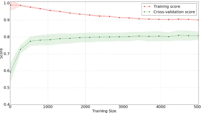
Figure 2. SVC Learning Curve with Best Unigram Features ... 52
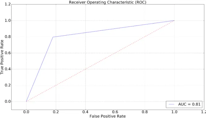
Figure 3. SVC ROC Curve with Best Unigram Features ... 53
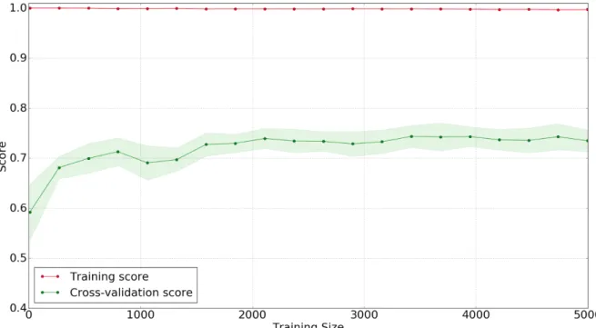
Figure 4. LinearSVC Learning Curve with Best Unigram Features ... 55
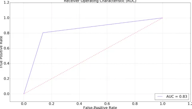
Figure 5. LinearSVC ROC Curve with Best Unigram Features ... 55
Figure 6. Logistic Regression Learning Curve with Best Unigram Features ... 57
Figure 7. Logistic Regression ROC Curve with Best Unigram Features ... 58
Figure 8. Decision Trees Learning Curve with Best Unigram Features ... 60
Figure 9. Decision Trees ROC Curve with Best Unigram Features ... 60
Figure 10. SGD Learning Curve with Best Unigram Features ... 62
Figure 11. SGD ROC Curve with Best Unigram Features ... 63
Figure 12. MNB Learning Curve with Best Unigram Features ... 64
Figure 13. MNB ROC Curve with Best Unigram Features ... 65
Figure 14. BNB Learning Curve with Best Unigram Features ... 67
Figure 15. BNB ROC Curve with Best Unigram Features ... 68
Figure 16. Random Forests Learning Curve with Best Unigram Features ... 70
Figure 17. Random Forests ROC Curve with Best Unigram Features ... 71
Figure 18. Gradient Boosting Learning Curve with Best Unigram Features ... 73
Figure 19. Gradient Boosting ROC Curve with Best Unigram Features ... 73
Figure 21. AdaBoost ROC Curve with Best Unigram Features ... 75
Figure 22. ERT Learning Curve with Best Unigram Features ... 77
Figure 23. Trump Account Token Distribution ... 87
Figure 24. Trump Campaign Team Token Distribution ... 88
Figure 25. Russia - Vladimir Putin Tweets Token Distribution ... 89
Figure 26. China Tweets Token Distribution ... 90
Figure 27. Syria-Iraq-Terrorism-ISIS Tweets Token Distribution ... 91
CHAPTER 1:
INTRODUCTION
Social science research community has a growing interest in the direction of quantitative models. Besides economics, there is a lack of reliable and accurate models in social science fields, and this is certainly true in International Relations and Political Science. There are several reasons behind it, but an important factor is the nature of the Social Sciences, it is difficult to quantify information that can be used in the state-of-the-art modeling techniques employed in natural sciences.
Today, we have much more data available than the social scientists in the past and much more opportunities to quantify and analyze social content and interactions. For example, hundreds of millions of people express their opinion freely and publicly in social media channels and these data and interactions are available to researches as raw data, regressable and analyzable linguistic features or network structures. With Machine Learning and Natural Language Processing algorithms, sentiment polarity of a post of a citizen or a policy decision maker can be analyzed probabilistically. Also, a decision maker’s network structure can be analyzed through her connections in a
social network to understand that decision maker’s policy orientation through not only her own data but with the data of her close environment as a whole.
Election forecasting is an interesting area which can be modeled using advanced data techniques due to availability of dependent and independent certain numerical measures (election results or opinion polls) that social scientist can crunch to produce reliable, accurate models and therefore predictions. Availability of social media medium data offers the chance of capturing voting intention on a very large scale, for example with millions of tweets from Twitter.
Being able to build quantitative models in elections is academically and practically valuable not just for its usefulness in the area of election forecasting but also for the advancement of social sciences in general, in terms of its reliability, accuracy and methodological plurality.
In International Relations, public opinion is a key element to scholarly analysis especially in some theoretical approaches and schools of thought. This work stipulates that decision making in international arena and conduct of foreign policy are directly dependent on the key people in the governments, which are elected by electorates' votes in ballot box in democratic countries, and their strategic interactions. Therefore, leaders and governments those leaders head are very important parameters in deciding how international relations evolve in time for the research community and politicians. Also, after the election and key decision makers assume take their
governmental positions, public opinion continues to exert its influence on decision making process. Decision makers, because of the audience cost and their prospective
domestic and foreign policy. Therefore, being able to predict and forecast which political party (or parties) will run a country or which leader will be the next
president, or more generally keeping track of the public opinion are fundamental to an accurate foreign policy analysis. To achieve the research objectives, this work focuses on both sides of the international - domestic nested game, the mutual dependency between foreign and domestic policies.
Domestic Politics: Election Forecasting through citizens voting intentions of 1 November 2015 Turkish general election and US presidential primary elections in 2016 using Twitter data
International Relations: Foreign Policy Topic Analysis through foreign policy orientation of US presidential election winner, president-elect Donald Trump’s campaign teams’ Twitter data during the campaign season
1.1 Domestic Politics, Election Forecasting
Current election forecasting methodologies differ in terms of their data and their emphasis on qualitative or quantitative models. There are four major types of election forecasting approaches according to (Lewis-Beck and Stegmaier, 2014):
1. Structuralist: Static, usually single equation models 2. Aggregative: Aggregate results from polls
3. Expertise on the domain: Depends on expert qualitative knowledge and intuition 4. Synthesizers: Combining polls data with structural features
We can define social media analysts as the fifth type which captures voting intentions of electorates from social media data using Facebook, Twitter, etc. This thesis does social media analysis and proposes a novel approach which combines Natural Language Processing and Machine Learning approaches to determine the voting intentions of electorate probabilistically in a statistically confident interval. The cases for election forecast methodology are Turkish 1 November 2015 general election and US primary elections in 2016.
1.2 International Relations, President-Elect D. Trump’s Policy Orientation
In the US Presidential Election of November 8, 2016, Trump was elected the president for 2017-2021 period. By assuming campaign team members hold key positions in administrative and governmental positions in successive presidencies, this work analyzes the twitter timelines of key members of Trump campaign team and Trump himself, in several important foreign policy issues for USA:
• Russia • China
• Syria – Iraq - Terrorism – ISIS • Iran
1.3 Main Research Objectives and Questions
1) Can we create a quantified model which can capture the voting intentions of electorate and over performs current methodologies used in the research community? How reliable are these current applied methodologies?
2) Can we create a model capable of explaining a decision maker’s policy orientation on specific issues during the campaign through their own twitter posts and network structure?
To be able to answer the questions given above from a collect ion of twitter data, we should be able to capture a tweet’s meaning in terms of sentimental polarity (positive vs. negative) for a specific policy issue accurately in a probabilistic model. Therefore, our third research question is:
3) In how much accuracy a tweet’s sentimental polarity (positive vs. negative) can be captured?
1.4 Research Approach
This work assumes social science issues can be analyzed and predicted by increasingly advanced computational and mathematical approaches applied on relevant datasets. Therefore, it focuses on machine learning, natural language processing, statistical algorithms and approaches to build models for forecasting elections and foreign policy choices.
1.5 Thesis Outline
Because this work is transdisciplinary and makes predictive analysis for international relations - foreign policy and to achieve this aim creates models using machine learning and natural processing from computer science, first, an extensive review of related literatures from these fields are provided. Methodological choices are
represented afterwards. Because sentiment analysis is at the core of the underlying model, results are discussed in detail especially for the Turkish sentiment polarity analysis to represent the process of algorithmic development. Therefore, English sentiment analysis will be given in less detail. After creating models, Turkish 2015 General Election and US 2016 Presidential Primaries will be analyzed and discussed. In the last case, Donald Trump’s campaign team’s discussion of several foreign policy issues will be discussed by analyzing his key campaign team members’ tweets.
CHAPTER 2:
LITERATURE REVIEW
In this section, election forecasting literature, leadership public content analysis literature and related sentiment analysis literature will be reviewed.
2.1 Political Science Election Forecasting Literature
In the current literature, election forecasting can be categorized into five different labels: Structuralists, Aggregators, Synthesizers, Experts (Lewis-Beck and Stegmaier, 2014), and Social media analysts. Because experts rely on their private knowledge, intuition and not on modeling this work does not discuss on them.
The Structuralists (Abramowitz, 2012; Campbell, 2014; Lewis-Beck and Tien, 2014) present a theoretical model of the election outcome with generally core political and economic parameters such as GDP growth, incumbency or attrition amount a running party burdens. The unit of analysis is either nation or district, based on the available granularity of the data. Estimation is done through regression and resulting function is static rather than dynamic.
The Aggregators, on the other hand, (Blumenthal, 2014; Traugott, 2014), aggregate vote intentions in opinion polls like Real Clear Politics. Voter preferences are combined over multiple polls and weighted according to their past historic performance and recency. Aggregators do not offer a theory which means not causal streams but correlation among independent and dependent variables important. Here accuracy of the forecast is the key not underlying theory. Because aggregators have access to polls result over a period they have the ability to create time series and update their forecasts.
The Synthesizers (e.g. Bafumi, Erikson, et al., 2014; Linzer, 2014) combines methods of the Structuralists and the Aggregators. Their work begins with a political economy theory of the vote and use aggregated and ongoing polling preferences as well. Analysis may include multiple equations and done on national or district level.
Social media analysts, in comparison, use publicly available user intentions and opinions, create metrics and crunch on the numbers. These kinds of works claimed social media data allows a reliable forecast of the final result (Sang & Bos, 2012). Some of these works rely on very simple naïve techniques, focusing on the volume share of the data related to parties or candidates. Along the same line, some scholars claimed that the number of Facebook supporters could be a good indicator of election results (Williams & Gulati, 2008), while Tumasjan, et al., 2011) compared party mentions on Twitter with the results of the 2009 German election and argued that the relative number of tweets related to each party is a good predictor for its vote share.
Some scholar criticized this kind of mere volume works and argued number of mentions or retweets, or the number of “like”s are crude ways of trying to forecast future (Gayo Avallo, et al., 2011). Some studies tried to improve this simple analysis by conducting sentiment analysis. Lindsay (2008), for example, built a sentiment classifier based on lexical induction and found correlations between several polls conducted during the 2008 presidential election and the content of wall posts available on Facebook. (O’Connor, et al., 2010) show similar results displaying correlation between Obama’s approval rate and the sentiment expressed by Twitter users. In addition, sentiment analysis of tweets proved to perform as well as polls in predicting the results of both the 2011 (Sang, et al., 2012) and the 2012 legislative elections in the Netherlands (Sanders, den Bosch, 2013), while the analysis of multiple social media (Facebook, Twitter, Google, and YouTube) was able to outperform traditional surveys in estimating the results of the 2010 U.K. Election (Franch, 2013).
However, other scholar argued that because just successful works are
published, predictions from social media should not be taken reliable (GayoAvello, et al., 2011; Goldstein & Rainey, 2010; Huberty, 2015). For instance, it has been shown that the share of campaign weblogs prior to the 2005 federal election in Germany was not a good predictor of the relative strength of the parties insofar as small parties were overrepresented (Albrecht, et al., 2007). In a study on Canadian elections, Jansen and Koop (2006) failed in estimating the positions of the two largest parties. Finally, Jugherr, Ju¨rgens, and Schoen (2012) criticized the work of Tumasjan et al. (2011), arguing that including the small German Pirate Party into the analysis would have yielded a negative effect on the accuracy of the predictions. Gayo-Avello (2011)
argues that several theoretical problems with predicting elections based on tweets. First, he stresses how several of the quoted works are not predictions at all, given that they generally present post hoc analysis after an election has already occurred. This also increases the chances that only good results are published, inflating the perceived ability of using social media to correctly forecast election. Second, he underlines the difficulty to catch the real meaning of the texts analyzed, given that political discourse is plagued with humor, double meanings, and sarcasm. Third, he highlights the risk of a spamming effect: Given the presence of rumors and misleading information, not all the Internet posts are necessary trustworthy. Finally, in most of the previous studies, demographics are neglected: Not every age, gender, social, or racial group is in fact equally represented in social media. This study responses to the criticisms made by Gayo-Avello in the limitations chapter.
There are also other papers in the Turkish social media analysis literature which do not focus on election forecast in general, but touches upon special cases in political matters in Turkey. Among this, there is Yenigun, G. E., 2013 that analyzes political mobilization and alliance structures in social networks. There is also reports by ORSAM like the one which works on tweets of terrorists in Turkey1. However, in current Turkish social media literature focusing on social media political matters, there is no study which works millions of tweets gathered via Twitter stream API and applies Machine Learning and Natural Language Processing algorithms.
2.2 International Relations FPA Through Decision Makers
This work focuses primarily on specific foreign policy issues discussed by the President Elect Donald Trump himself and his campaign team during the 2016 US Presidential Election by analyzing their tweets. There are “personality at distance” approaches in Foreign Policy Analysis literature, which, like this work, analyze leaders’ speech or interview contents although they model personalities of leaders in general not their orientation for specific foreign policy issues.
In Foreign Policy Analysis, “personality at a distance” analytical approaches to determine leadership styles, in decision making process occupy an important place (Hermann, 1977). Leaders’ interviews, speeches, behavior and past experiences, biographies and autobiographies are all analyzed to make this kind of analysis.
Of these several approaches, Operational Code (OpCode) ((George, 1969) and Leadership Trait Analysis (LTA) (Hermann, 1977). uses decision makers’ speeches and answers to interview questions, respectively, as their working material. They are closely related, share some parameters and differ in some aspects. This work enhances prediction capabilities of both of these statistical, related approaches via new channels of information we have in today’s world (social media data).
LTA and OpCode focuses on grand personality features, an approach which does not focus on specific foreign policy issues. Besides using twitter data of decision makers and their campaign teams as new sources, another novelty of this work is, it directly analyzes specific foreign policy issues instead of personalities. Because there
is no relevant literature focusing on these two aspects, above mentioned two most well-known approaches, LTA and OpCode will be reviewed briefly.
2.2.1 Leadership Traits Analysis
Leadership Traits Analysis, models leaders’ propensities analyzing their answers to the interview questions and calculate values for the parameters: Control over Events, Need for Power, Conceptual Complexity, Self-Confidence, Task Orientation, Distrust of Others and In-Group Bias (Hermann, 1977). LTA focuses on interviews because it sees them more spontaneous than public speeches which may be written by leaders’ advisers or speech writers (Hermann, 1977)
LTA uses verbs or other words (adjectives, pronouns etc.) to calculate the measures for the parameters. For accurate LTA analysis, at least 50 interview responses with at least 100 words are needed. These interviews should span through leaders’ the term in the office and should be on variety of topics and spontaneity levels.
2.2.2 Operational Code
Operational Code first developed by Leites in 1951 in Rand and then redeveloped (George, 1969). It models typology and personality of leader (Walker, 1998).
calculations on the speech material of those decision makers and “asks what the individual knows, feels, and wants regarding the exercise of power in human affairs” (Schafer & Walker, 2006). To do so it focuses on two sets of variables sets,
philosophical ones and instrumental ones (George, 1969) and (Holsti, Rosenau, 1979):
“P-1. the fundamental nature of politics, political conflict, and the image of the opponent;
P-2. the general prospects for realizing one's fundamental political values P-3. the extent to which the political future is predictable
P-4. the extent to which political leaders can influence historical developments and control outcomes
P-5. the role of chance? What are the leader's instrumental propensities for choosing? I-1. the best approach for selecting goals for political action, i.e., strategy
I-2. how such goals and objectives can be pursued most effectively, i.e., tactics I-3. the best approach to calculation, control, and acceptance of the risks of political action
I-4. the "timing" of action"
1-5. the utility and role of different means?” (Walker, et al., 1998)
In calculating these propensities, our main parameters are leaders’ attributions to themselves (to their individual beings) and to the others, positively or negatively. To understand whether a verb (which is what we focus) is positive or negative, Verbs and Context System (VCIS) is used. Verbs in context system codes verbs according to verbs’ subject, time and category. It also looks at domain and the context.
2.3 Sentiment Analysis Literature
Sentiment Analysis, also known as Opinion Mining, is the use of Natural Language Processing, text analysis and computational linguistic techniques with the help of Data Mining and possibly Machine Learning to extract meaning from text data. Because of much more available public and free data on the Internet, sentiment Analysis has gained a lot of interest in the recent years.
Sentiment Analysis works have been done on a wide range of fields such as movie reviews (Pang et al., 2002), product reviews and news and blogs (Bautin et al., 2008) and they can be broadly categorized into three classes:
Polarity: Documents are categorized into positive, negative and neutral.
Emotion: This works focus on emotions or mood states expressed in documents, such as happiness, joy, surprise, among others.
Strength: As a cross-cutting feature, polarity and emotion based classification can be carried out with strength values attached, like numerical scores showing the level of positivity or joy.
Although in Sentiment Analysis, there are less categories than topic classification, it is considered as a harder field of Natural Language Processing because usually sentiment is represented on at least sentence level instead of topic classifiers dependence on words. Therefore, for a successful sentiment classification, it is necessary to analyze words in their order in domain also considering their potential expression with irony, sarcasm and negation. (Pang and Lee, 2008)
Although in polarity based sentiment analysis, texts can be categorized into subjective (positive, negative) and objective (neutral) classes in terms polarity, in Tweet sentiment analysis, most studies assume the subjectivity of the text, therefore focuses on positive and negative labels.
In terms of classification methodology, there exists two different paradigms: Sentiment Analysis (SA) with Lexicons [aka Knowledge Based] and SA with Machine Learning. The lexical approach utilizes a dictionary of words tagged with sentimental polarity; positive, negative or neutral. Some lexicons use has been built on word’s emotional context such as happiness, excitement etc. Works using lexicons, compare words in their corpus to the words in the lexicons. sentiment meaning, then, is computed by counting positive and negative words in a sentence (or in a document, depending on the level of granularity of the classification) and if the number of positive words is greater than the number of negative ones, then that sentence is labeled is positive otherwise negative. Some lexicons have also strength value in a scale attached to the words. In this case, sentiment labeling of that sentence is done through the summation of weighted word polarity values by their strength value. It is also possible to use supervised machine learning for modeling sentence level
aggregated polarity values by taking them features and annotated sentence polarities as the labels.
There are several lexicons used in sentiment analysis such as OpinionFinder (OPF), Affective Norms for English Words (ANEW), AFINN, SentiWordNet, WordNet, SentiStrength, NRC, and others. The problem with lexical sentiment analysis is the fact that it does not take into account of twitter jargon. Because words
used in Twitter do not adhere the rules of formal language, it is possible that many words in Twitter corpus escape the matching process between tweets and a lexicon. These types of words include Twitter slang, informal abbreviations, grammatical mistakes etc. Although with extensive preprocessing and stemming (in Turkish for example), this problem can be solved in some degree, this solution can’t catch the sentiment meaning of that words in the context of their usage. To be able to capture the sentiment meaning of a word in relation to other words in a sentence (or a document), sentence (or document) level analysis is required.
The other paradigm in sentiment analysis, namely using machine learning, requires supervised and unsupervised approaches, however unsupervised algorithms only capture the sentiment meaning to some degree and is used for some auxiliary work such as topic classification by Latent Dirichlet allocation (LDA), Latent Semantic Analysis (LSA) or vector representation by Word2Vec. In supervised approach, on the other hand, labeled data is needed and that can be built by manual annotation or by distant supervised methods such as labeling from emoticons or hashtags. A commonly used method is labeling tweets containing “:)” as positive and “:(“ as negative.
2.3.1 Sentiment Analysis in Twitter
Sentiment analysis of tweets are especially more difficult than long, informal texts such as blog posts because: (Martinez-Camara et al, 2014)
1) Tweets are informal in the sense that they have lots of abbreviations, internal slang and its has its own style of jargon.
2) Grammar of tweets is problematic. Many users do not care about the grammatical correctness of text. Twitter’s policy of maximum text length of 140 plays important role here.
3) Users refer to the same concept via different words, abbreviations and irregular forms. Because of this, same concepts usually get represented by different words, which creates data sparsity problem. If not handled, this problem creates performance issues in sentiment analysis classifiers.
4) Because tweets are short, identifying their context is difficult conceptually and computationally, meaning a token’s previous and successive tokens are few.
One of the earliest studies of tweet sentiment analysis was a classification of tweets, in English, by supervised machine learning algorithms (Go, Bhayani, Huang, 2009). Their work was on a dataset collected through Twitter Search API and labeled through the existence of emoticons ( “:” for positive, “:(“ for negative ). That work’s results showed that, supervised algorithms are the best approach for sentiment
analysis, POS (Part of Speech) tags are irrelevant in tweet classification and unigrams works quite well in short text as opposed to long documents. Furthermore, they found that predictive accuracy can be improved slightly by using a combination of unigrams and bigrams. Another work (Kim et al. 2009), uses not machine learning but uses the Affective Norms for English Words (ANEW) lexicon to capture emotion sentiment.
Pak and Paroubek (2010), in their work, annotates tweets in their dataset with emoticons for positive and negative labels. Also, they collect neutral tweets from the
official twitter accounts of newspapers and magazines. At the modeling step, they use supervised machine learning algorithms: Conditional Random Fields (CRF), Support Vector Machines and Naive Bayes. They conclude that n-grams, POS tags and Naive Bayes are the best the configuration for accurate classification.
Thelwall, Buckley and Paltoglou (2011) focuses on the intensity of tweet sentiments. For this purpose, they use SentiStrength lexicon which assigns a score for positivity and negativity on a strength scale of 1 to 5. Their conclusion is sentiment strength is a useful predictor for learning the behaviors of twitter users.
Khan et al. (2015) uses a hybrid approach and uses a machine learning algorithm, support vector machine, after assigning each tweet using the lexicons. They found that turning abbreviations into whole words, removal of links, POS tagging, deleting retweets and modeling with SVM results in accurate models.
Barbosa and Feng (2010), theorized that just using n-grams can decrease predictive power due to existence of large number of infrequent words in Twitter because of grammatical mistakes. They proposed, instead, inclusion of Twitter and microblogging specific features such as mentions, emoticons, punctuations, retweets and hashtags. In their work, using this enlarges set of features improved accuracy 2% in Support Vector Machine classification. A similar approach was advised by
Kouloumpis, et al, (2011) with the addition of abbreviations and intensifier words as features. They showed that best performance in their work was achieved by a
combination of prior probability of words, n-grams, Twitter specific and lexicon polarity features. However, POS tags decreased the predictive accuracy.
Davidov, Tsur and Rappoport (2010) uses hashtags and emoticons as instance features and models them with K-Nearest Neighbors (KNN) algorithm with promising results. In a comparative study by Agarwal et al. (2011), using unigrams, tree-based models, partial tree kernels and several combinations of them. They assign polarities to words in tweets using DAL dictionary. They conclude that, based on comparison of their results with other research, numerical word polarity based methods are superior to the others. Bifet and Frank (2010) uses data flow algorithms and Kappa evaluation measure on sentiment classification besides three machine learning algorithms, Multinomial Naive Bayes, Stochastic Gradient Descent (SGD) and Hoeffding tree. Their results show that accuracy of SGD is better than the others.
Hernández and Sallis (2011) uses an unsupervised algorithm Latent Dirichlet allocation (LDA) although they do not classify tweets based on sentiments. They just show that vector representation of tweets after LDA analysis and Tf-Idf weighting has less entropy therefore these methods can give better results when combined with classification algorithms. Aisopos et al. (2012) uses character n-grams to solve the problems with Twitter data mentioned above. Because on character level every text is independent of language, sarcasm and irony, grammatical errors and language style becomes irrelevant. They found their supervised model shows good performance. Martinez-Camara et al, (2014) gives a good summary of existing works on Twitter sentiment analysis with their accuracies when available.
CHAPTER 3:
BACKGROUND THEORY AND METHODOLOGY
3.1 Background Theory
This work, to forecast elections and foreign policy, creates models by building upon novel machine learning (ML) and natural language processing (NLP) algorithms and techniques. In this section, related background ML and NLP definitions, concepts, theories, algorithms and approaches are discussed.
3.1.1 Machine Learning
“The field of machine learning is concerned with the question of how to construct computer programs that automatically improve with experience.” (Mitchell, 1997) As a shortly formalized version:
“A computer program is said to learn from experience E with respect to some class of tasks T and performance measure P, if its performance at tasks in T, as measured by
Machine Learning algorithms are data driven, meaning they are algorithms which create other algorithms’ steps through their dataset. For example, in this work’s case: sentiment analysis is not done by writing the rules of extracting sentiment meaning from sentence but modeled through the dataset which is annotated for this work. The main aim of a machine learning algorithm is building a probabilistic model which in essence an algorithm.
Machine Learning algorithms has two main approaches in terms of learning style:
Supervised
In supervised machine learning, instances in the dataset are labeled to give directions to the algorithms. In this work’s case, sentences in the dataset are labeled as positive or negative manually by the humans (or neutral which are filtered out before training stage).
Unsupervised
Unsupervised machine learning algorithms create models from a dataset of unlabeled instances. They do not need human assistance for classification. Main uses of unsupervised methods are clustering and feature engineering.
Supervised and unsupervised approaches can be mixed to create intermediate forms and they are called semi-supervised algorithms. In this work, classification through Doc2Vec, is that kind of machine learning in which first vector
using Word2Vec on word level, another unsupervised algorithm) in unsupervised fashion, and then these vectors are fed into supervised algorithms.
3.1.1.1 Machine Learning Terminology
In this chapter, fundamental machine learning terminology and concepts will be defined.
Training data
The data we have (labeled or unlabeled), to feed into the machine learning algorithms. The algorithms learn models from the training data.
Test data
The models leaned by the algorithms are, tested against the test data. Test data and training data are assumed to be disjoint.
Instances and their features
Each member of the training and testing dataset is called an instance. So, for a supervised algorithm, a row in the training set is composed of instance with its label. The properties of an instance are its features.
Sparse Matrix
In machine learning, instances and their features are represented as matrices whose rows are instances and columns as features. In NLP, due to high number of features because of high number of words and misspellings, many (instance, feature) pairs are just empty in the matrix representation. Therefore, these empty pairs are dropped from the matrix to decrease memory usage. This representation is called the
Classes
Classes, aka labels, are the categories which training instances belong to. In sentiment analysis, classes can be positive, negative, neutral, or some emotional categories such as happiness, excitement etc.
Table 1. Sentiment Examples
Instance Class
Today is Monday. Neutral
Weather is excellent today. Positive
What a bad country. Negative
Training
A classifier said to be trained on the training dataset when it creates a model from the training instances.
Classification
Classification means assigning an instance of a test dataset to a class label such as assignment of a tweet to positive class.
Classifier
The model, built upon the training data, which assigns class labels to instances are called classifier or estimator because of its probabilistic nature.
Feature Engineering and Feature Selection
Although instances may have many features, just a subset of them may be relevant or sufficiently predictive for an accurate and computationally efficient classification task. Determining which subset is optimal for an accurate modeling is
called feature selection. Sometimes, new features may need to be defined from existing ones by combining them. The process of feature selection and creating new features from existing ones is called Feature Engineering.
Learning Curve
Learning curves are used to plot the relationship between number of training instances and the performance of a classifier. It is a great way to show how an information processing algorithm learns with experience.
3.1.1.2 Machine Learning Algorithms
In subsequent sections; the terms “algorithm”, “classifier” and “model” are used interchangeably. Also, “label” and “class” have same meanings.
3.1.1.2.1 SVM
Support Vector Machines (SVM), (Cortes and Vapnik, 1995), builds a decision surface with a set of hyperplanes on the borders of training instances (support vectors) whose locations in the instance space gives the optimum margin to differentiate members of different classes.
The key idea behind SVM’s are if training instances are not linearly separable in their n dimensional space, then in a hyperspace with higher than n dimension, there can be found hyperplanes which separates the instances optimally. This approach is
Sigmoidal, linear and Polynomial Kernel. Furthermore, an SVM model with a kernel (similarity function) is analogous to two-layer Neural Network with a different cost function (as the first layer to project data into another space, and second layer to classify). SVM algorithm can also be used for classification problems with more than two classes. In these cases, usually, one-again-rest or one-against-all methods are used.
Advantages of SVM’s are:
• They are effective in high dimensional spaces which is characteristic in text classification.
• Uses a subset of training instances (support vectors) in the decision function, therefore it is memory efficient.
• It can use custom kernel functions (similarity measure) specific to needs (this kernel function determines the distance among instances in the space)
3.1.1.2.2 Logistic Regression
Logistic Regression classifiers regress the training data but by using a threshold they assign classes (discrete values) to instances instead of regression algorithm’s
continuous outputs, their dependent variables are categorical.
Although logistic regression is special kind of generalized linear regression, it assumes conditional probabilities have Bernoulli distribution instead of Gaussian distribution. In addition, Logistic Regression is equivalent to Maximum Entropy
modeling (Mount, 2011), their decision functions can be derived from each other. However, there are several implementations of Maximum Entropy classifiers using different underlying algorithms, in turn, have different accuracies on their
classification problem.
The logistic regression algorithms are a widely successful algorithm in a wide range of domains such as topic classification, sentiment analysis and language
detection.
3.1.1.2.3 Decision Trees
Decision trees classify instances by hierarchically sorting them through their feature values. Nodes refer to features while leaves are classes. At each tree level, best feature in terms of its ability to differentiate instances, is selected for the nodes. Most
commonly used methods for selecting best features are entropy and information gain. Feature selection continues until a level is found where all instances have the same labels (stop conditions). After the training step, a new instance is classified by going through the root of three till a class label is found.
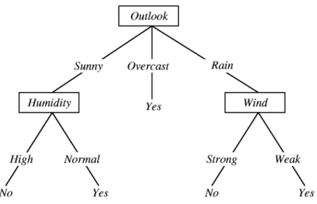
Figure 1. A sample decision tree (Mitchell, 1997)
A decision tree can be seen as a condensed version of a rule table. Each path from root to the leaves is a rule of the model and leaves are the categories in which training instances fall into.
3.1.1.2.4 Stochastic Gradient Descent
Gradient descent (or ascent) algorithms try to approximate maximum or minimum of an objective function (aka decision, loss, error or cost function) in a large problem space which is computationally very expensive to trace every corner of it. Stochastic gradient descent, on the other hand, is the stochastic approximation of the Gradient Descent, which optimizes the parameters of objective function by one training sample at a time, in each iteration. It is widely used in text classification problem which requires lots of features, and is very efficient in terms of computational cost. Another
advantage of Stochastic gradient descent algorithm in Natural Language Processing tasks is its capability in sparse data problems.
3.1.1.2.5 Maximum Entropy Classifier
Another well-known technique for Natural Language Processing is Maximum Entropy algorithm (Nigam et al. 1999) and its varieties that produce a discriminative model by learning soft or hard boundaries between classes in the instance space (similar to SVM and decision trees) as opposed to generative models which model the underlying distribution of training data (such as Naive Bayes algorithm). Maximum Entropy Classifiers do not assume, unlike Naive Bayes classifiers, features are conditionally independent of each other. Its underlying assumption is the Principle of Maximum Entropy which states that maximum information gain can be realized through the model that has the maximum entropy (entropy means the unpredictability of an information content) if we do not know the underlying distribution of an event.
Maximum entropy classifiers need more time than Naive Bayes classifiers because they first need to solve internal optimization problem to find parameters of the model. There are several training methods for Maximum Entropy classifiers such as GIS, IIS and Megam (Daumé III, Hal., 2004)
3.1.1.2.6 Naive Bayes
Naive Bayes classification algorithm rests upon the Bayesian Theorem which can be, in our case:
P(class | feature) = P(class) * P(feature | class) / P(feature)
with the meaning that probability of a class (positive or negative) of a given the feature is dependent on prior probability of that class, probability of seeing that feature given the class and probability of that feature in the corpus. Naive Bayes classifier builds upon this idea and considers every feature independent of other features.
In a document d, the assignment of class c to d is done by calculating the probabilities of each class given the document, then selecting the Maximum Posterior Probability (MAP) estimate:
c MAP = argmax Pc∈C (c|d) using the Bayesian Formula, then c MAP = argmaxc∈C P (d|c) × P (c) / P (d) because P(d) is independent of and same in each class
c MAP = argmaxc∈C P (d|c) × P (c) if we show a document with feature set,
d = f1,f2,f3,f4,,,fn
which makes our Naive Bayes classifier formula as: c NB = argmaxc∈C P (c) ∏a P (a|c)
Naive Bayes classifiers can be differentiated according to underlying probability distribution of p(feature | class) such as Multi-variate Bernoulli Naive Bayes, Multinomial Naive Bayes or Gaussian Naive Bayes.
In certain domains, it has been showed that Naive Bayes algorithm can perform better than more complex algorithms such as Neural Networks (Mitchell, 1997).
3.1.1.2.7 Ensemble Methods
Ensemble learning use multiple classifiers and combines their results for better predictive accuracy. The aggregate result can be calculated by majority rule voting or sum of the predicted probabilities for each of the class label. Voting and summation can be done using a weighted schema by giving not uniform weights for classifiers.
3.1.1.2.7.1 Random Forests
Random Forests classifiers, as an ensemble method and meta estimator, use a set of decision trees and combines their results for a given example to predict. Its
assumption is by building n number of decision trees each trained with a subset of the training data set (bagging – bootstrap aggregating), totality of all trees can have higher accuracy than a single decision tree trained on the whole data set.
3.1.1.2.7.2 Gradient Boosting Classifier
“With excellent performance on all eight metrics, calibrated boosted trees were the best learning algorithm overall. Random forests are close second.” (Caruana, 2006)
Gradient Boosting Classifiers, like Random Forest models, uses decision trees. Instead of Random Forest’s approach of estimating with full blown trees, Gradient Boosting Trees are weak learners with high bias and low variance. The algorithm, in a forward-stage-wise fashion incrementally improves the trees by mainly reducing bias but also, to some extent, variance by aggregating the predictions of weak decision trees.
3.1.1.2.7.3 Extremely Randomized Trees Classification
Extremely Randomized Trees classification first fits randomized decision trees (in other word extra trees) on sub samples of whole dataset. Then, it aggregates results of sub trees to improve predictive power and reduce bias. Although similar, there are two main differences between Extra Trees and Random Forests which are:
- Extra Trees use sub samples from the whole training data set instead of bootstrap of the training data in each split stage while in a Random Forest meta estimator, each decision tree works specifically on a subset of the data (bagging – bootstrap aggregating)
- In each component tree, splits are chosen randomly which involves extra randomness in the ensemble, meaning components trees’ mistakes are less correlated to each other.
3.1.1.2.7.4 Adaptive Boosting Classifier
Adaptive Boosting algorithm (Freund et al, 1999) is an meta estimator as an ensemble method, begins by fitting a classifier on the original whole training dataset. Then, each cycle by increasing the weights of the wrongly classified instances, AdaBoost fits the base classifier. By focusing on the wrongly classified instances in successive steps, it tries to reduce error rate.
3.1.1.3 Classification Evaluation Criteria
In this work, performance of Machine Learning algorithms will be presented comparatively by using the evaluation criteria mentioned below.
3.1.1.3.1 K-fold Cross Validation
Cross validation (aka rotation estimation) is a model validation technique to measure the generalization capability of a model learned from training dataset to out-of-sample instances. In K-fold Cross Validation, training dataset is divided into k separate subsets and with each (k-1) of them, model is trained to predict the remaining subset.
Therefore, there are k possible subsets and in each k iteration, a different (k-1)
combination is selected for training. To calculate overall model predictive accuracy, k accuracies are averaged to get a smooth precision and decrease the weight of possible outliers. In this work, k is chosen as 10 which is the most common value in the literature.
3.1.1.3.2 Precision
Precision, aka positive predictive value, represents the exactness of a classification system. It is defined as (True Positives) / (True Positives + False Positives), in other words, number of correct positive results divided by the number of all positive results.
3.1.1.3.3 Recall
Recall, aka sensitivity, represents the completeness of a classification system. It is defined as (True Positives) / (True Positives + False Negatives), in other words, number of correct positive results divided by the number of positive results that should have been returned (all positive results in the dataset but not returned by the classifier).
3.1.1.3.4 F1-Score
F1-Score incorporates both precision and recall by using both in its formula. F1 is the harmonic mean of precision and recall:
3.1.1.3.5 Roc and Auc
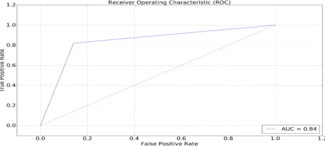
Receiving Operator Characteristic (ROC) Curve and Area under Receiving Operator Characteristic Curve (AUC) are used to illustrate the performance of a classifier ranking function. ROC is plotted as True Positive Rate (recall, sensitivity) against False Positive Rate (1 – specificity).
3.1.1.3.6 Training Score and Testing Score
Training score is the accuracy which the classifier performs in the training data after it is fitted. Testing score is the accuracy of the classifier in the testing data. When
precision is mentioned for a classifier, it corresponds to the testing score. However, training score is also very important, because a classifier with a very high training score is in the danger of overfit. Therefore, classifiers with high and similar testing and training scores can be said to have optimal configuration, probabilistically.
3.1.2 Natural Language Processing (NLP)
In this work, several NLP methods and text representations were used to be able to decide which ones are suitable for Turkish and English in terms of their contribution to the sentiment analysis accuracy.
3.1.2.1 N-gram model
N gram model of text is probabilistic language model to predict the next token given the tokens specified. It is highly used in NLP and Information Retrieval fields. N can be 1,2, 3... etc. As an example, the sentence “the United States is a member of United Nations” can be represented in:
Unigram (1-gram): “the”, “united”, “states”, “is”, “a”, “member”, “of”, “united”, “nations”.
Bigram (2-gram): “the united”, “united states”, “states is”, “is a”, “a member”, “member of”, “of united”, “united nations”.
3.1.2.2 Bag of words (bow)
A bag of words can be considered as a set in which each member is attached with its frequency. In our example “the United States is a member of United Nations” corresponding bow representation is:
“the:1, united:2, states:1, is:1, a:1, member:1, of:1, nations:1”
3.1.2.3 Tf-Idf
Tf–Idf, term frequency–inverse document frequency, is a widely used weighting method in Information Retrieval and NLP communities. It gives more weights proportionally to terms in a dataset which occurs in a document more frequently but offset by term’s occurrences in the whole corpus. Therefore, a term which is seen frequently in small number of documents has higher Tf-Idf value than a term which is
sprawled over entire corpus. As a result, terms with higher discriminating value for document or sentence classification is rewarded by Tf-Idf. Although there are several implementations of Tf-Idf a classical formula of it is:
w(i,j) = tf (I,j) * log(N / dfi) where
tf j,j = number of occurences of I in document j df I = number of documents containing term I
N = total number of documents in the corpus
3.1.2.4 Word2Vec and Doc2Vec
Word2vec (Goldberg et al, 2014) is a shallow neural network to produce vector outputs for given words. This is achieved through transforming each word in the text into n-dimensional (a parametric variable number) continuous vector space by analyzing distributional properties of that token in the document. As an unsupervised algorithm, word2vec does not need labeled data, creates word embedding model by analyzing corpus (set of documents) and extracting token distribution through cbow and skipgram (Levy et al, 2015) as explained below.
3.1.2.5 Cbow (continuous bag of words)
Uses bag of words approach mentioned above. The goal of the word2vec shallow neural network which uses cbow is to maximize P(token|context), meaning predicting
3.1.2.6 Skip-gram
It is similar to n-gram but skips some tokens so its components are not consecutive in the text. For example, in the text “the United States is a member of United Nations”, 1 skip 2grams are: “the states, united is, states a, is member, a of, member united, of nations”. When word2vec model initialized with skip-gram, it maximizes
P(context|token), in other words it predicts the context given the word.
“The skip-gram method weights nearby context words more heavily than more distant context words.” (Mikolov, et al, 2013). Therefore, although Cbow is faster than skip-gram, skip-gram gives higher accuracy for infrequent words.
In Word2vec, the model can be trained via negative sampling or hierarchical softmax are used. Negative sampling, minimizes the log-likelihood of sampled instances of PMI (Pointwise Mutual Information). On the other hand, hierarchical softmax algorithm uses Huffman trees to reduce calculation so it does not need compute the conditional probabilities of all vocab words. According to (Mnih et al, 2009) hierarchical softmax works better for infrequent words while negative sampling works better for frequent words.
Therefore, there are four combinations in a word2vec model, with two representation methods (cbow and skip-gram) and two training algorithms (negative sampling and hierarchical softmax). Doc2vec uses word2vec algorithm to vectorize not just words but also text chunks, sentences, paragraphs and documents by combining text’s word2vec representations.
3.2 Methodology
To build the election and foreign policy models, an advanced programming system is created. In this section, technical details of this system, data collection step,
preprocessing and annotation of tweets, high level statistical analysis of the dataset will be discussed.
3.2.1 System Design and Programming Environment
All data analysis and modeling were done using Python language using PyCharm as the IDE. In data collection step, tweets are stored in a text file each row corresponding to a tweet in json format (the format of Twitter API’s). In analysis stage, tweets were preprocessed and resulting reduced json format were stored in MongoDb because of its inherent support for json format and Python dictionary data structure. For Natural Language Processing, Gensim and NLTK libraries of Python were used. In the modeling step, for machine learning, Scikit-Learn (sklearn) was used (Pedregosa, et al, 2011).
Rationale behind System Design and Programming Environment
In all computational steps Python was used as the programming language. There are other alternative tools: R, Microsoft Office Excel, SaS, Wecka etc. However, Python combines two very important advantages:
• Availability of excellent statistical, machine learning and natural language processing packages with multi-core support (sklearn, gensim, nltk)
• Easiness of coding as a very high level language with higher abstraction compared to lots of other programming languages
As the database management system, NoSql MongoDb was used because of its excellent support for Twitter API’s json results and their corresponding Python dictionary data structure. Another reason for a NoSql Db was the Twitter API’s json results’ self-referential structure which is hard to represent and not natural in classical Sql Db’s such as MySql.
3.2.2 Data Collection
Tweets were collected from Twitter Streaming API with selected keywords. Data collection is done via Tweepy package (a wrapper for the rest based Twitter api, json based) and Python programming language. Twitter streaming API provides maximum 1% of all tweets randomly in real time, filtered by the set keywords. Although Twitter Gardenhouse API (10% of all tweets) and Firehouse API (100% of all tweets), these options are not free and for the work's purposes randomly selected 1% of all tweets is suitable. There is also Twitter Search API, which gives only a few days of data, therefore is not practical for the purposes of this work.
3.2.2.1 Keywords 3.2.2.1.1 TURKEY
akparti = ["adalet ve kalkınma", "akparti", "akp", "erdoğan", "davutoğlu", "@Akparti", "@RT_Erdogan", "@Ahmet_Davutoglu"]
chp = ["cumhuriyet halk", "chp", "kılıçdaroğlu", "@herkesicinCHP", "@kilicdarogluk"]
mhp = ["milliyetçi hareket", "mhp", "bahçeli", "@dbdevletbahceli"] hdp = ["halkların demokratik", "hdp", "demirtaş", "@HDPgenelmerkezi", "@hdpdemirtas"]
To collect tweets from Twitter API, keywords were selected carefully to not to introduce topic bias into the dataset. For each political party; name of the party, its abbreviation, surname of the leader of the party, official twitter accounts of both of the party and the leader were used. In Justice and Development Party (Akparty), President Recep Tayyip Erdoğan and Prime Minister Ahmet Davutoğlu were both considered as the party leaders because of electorates obvious perception of that. Also, due to widespread usages of akparti and akp as abbreviations, both of them were used. Furthermore, in Nationalist Movement Party, there is no official party Twitter account.
3.2.2.1.2 USA
Republican Presidential Candidates
trump = ["Donald Trump", "@realDonaldTrump"] cruz = ["Ted Cruz", "@tedcruz"]
rubio = ["Marco Rubio", "@marcorubio"] carson = ["Ben Carson", "@RealBenCarson"] kasich = ["John Kasich", "@JohnKasich"]
bush = ["Jeb Bush", "@JebBush"] Democratic Presidential Candidates
sanders = ["Bernie Sanders", "@BernieSanders"] clinton = ["Hillary Clinton", "@HillaryClinton"]
In US Presidential Primary Elections, again a formal procedure was used to select keywords for Twitter Streaming API. For each of the candidates, only their names and their official twitter account names were used. However, in this dataset, after the primary election results, only Trump’s and Clinton’s tweets are analyzed.
3.2.3 Preprocessing
Several steps for taken to modify tweet texts before modeling their sentimental polarity.
Lowercase characters
All tweets were lowercased. In Turkish example because of special characters (İ,Ü,Ç...etc.) first all characters were capitalized then lowercased to get uniform representation.
Json reduction
All fields from Twitter json data which are not needed were filtered out such as entities, places, url tags. A twitter json example:
{
"text": In preparation for the NFL lockout, I will be spending twice as much time analyzing my fantasy baseball team",
"favorited": false,
"source": "<a href=\"http://twitter.com/\" rel=\"nofollow\">Twitter for iPhone</a>", "in_reply_to_screen_name": null, "in_reply_to_status_id_str": null, "id_str": "5469180224328", "entities": { "user_mentions": [ { "indices": [ 3, 19 ], "screen_name": "X", "id_str": "271572434", "name": "X", "id": 271572434 } ], "urls": [ ], "hashtags": [ ] }, "contributors": null, "retweeted": false, "in_reply_to_user_id_str": null, "place": null, "retweet_count": 4,
"created_at": "Sun Apr 03 23:48:36 +0000 2011" }
Valid, invalid, spam types
Twitter API returns true tweets and sometimes HTTP status messages both in json content. All json messages labeled with either valid (true tweet), invalid (HTTP status message or broken messages due to network issues) or as spam.