ONLINE CHURN DETECTION ON HIGH DIMENSIONAL CELLULAR DATA USING
ADAPTIVE HIERARCHICAL TREES
Farhan Khan
1, Ibrahim Delibalta
2, Suleyman S. Kozat
11
Bilkent University, Ankara, Turkey
2
AveaLabs, AVEA Iletisim Hizmetleri A.S. Istanbul, Turkey
ABSTRACT
We study online sequential logistic regression for churn de-tection in cellular networks when the feature vectors lie in a high dimensional space on a time varying manifold. We es-cape the curse of dimensionality by tracking the subspace of the underlying manifold using a hierarchical tree structure. We use the projections of the original high dimensional ture space onto the underlying manifold as the modified fea-ture vectors. By using the proposed algorithm, we provide significant classification performance with significantly re-duced computational complexity as well as memory require-ment. We reduce the computational complexity to the order of the depth of the tree and the memory requirement to only linear in the intrinsic dimension of the manifold. We provide several results with real life cellular network data for churn detection.
Index Terms— Churn, big data, online learning, classifi-cation on high dimensional manifolds, tree based method.
1. INTRODUCTION
Online data classification is widely investigated in data min-ing [2], machine learnmin-ing [4] and churn detection in cellular networks [1]. For applications involving big data [2], when the input vectors are high dimensional, the classification mod-els are computationally complex and usually result in overfit-ting.
In this paper, we study non-linear logistic regression us-ing high dimensional data assumus-ing the data lies on a time varying manifold. We partition the feature space into several regions to construct a piecewise linear model as an approx-imation to the non-linearity between the observed data and the desired data. However, instead of fixing the boundaries of the regions, we use the notion of context trees [5, 6] to repre-sent a broad class of all possible partitions for the piecewise linear models. We specifically introduce an algorithm that in-corporates context trees [5, 6] for online learning of the high dimensional manifolds and perform logistic regression on big data.
This work has been supported in part by AveaLabs, TUBITAK TEYDEB 1501 no. 3130095 project.
In most modern applications, where high dimensional data is involved, learning and regression on the manifolds are widely investigated. For instance, in cellular networks [1], large amounts of high dimensional, time varying data of various users are used for churn detection. The problem of manifold learning and regression is rather easy when all the data is available in advance (batch), and lies around the same single static submanifold [8]. However, in online manifold learning, it is difficult to track the variation in data because of the high dimensionality and time varying statistical distri-butions [8]. Hence, we introduce a comprehensive solution that includes online logistic regression on a high dimensional time series.
Note that various approaches are studied for the dimen-sionality reduction as a preprocessing step for the analysis of the high dimensional data [8,9]. In our approach, however, we use context trees to perform logistic regression, which adapts automatically to the intrinsic low dimensionality of the data by maintaining the “geodesic distance” [7] while operating on the original regressor space. In the domain of online non-linear regression, context trees have been used to partition the regressor space hierarchically, and to construct a competitive algorithm among a broader class of algorithms [6]. However, we use hierarchical tree structure to track and learn the man-ifold in a high dimensional setting. In addition to solving the problem of high dimensionality by incorporating mani-fold learning, our algorithm also performs online logistic re-gression.
To this end, we introduce an algorithm that uses a tree structure to hierarchically partition the high dimensional fea-ture space. We extend the algorithm by incorporating ap-proximate Mahalonobis distance as in [8] to adapt the feature space to its intrinsic lower dimension. Our algorithm also adapts the corresponding regressors in each region to mini-mize the final regression error. We show that our methods are truly sequential and generic in the sense that they are indepen-dent of the statistical distribution or structure of the data or the underlying manifold. In this sense, the proposed algorithms learn i) the structure of the manifolds, ii) the structure of the tree, iii) the low dimensional projections in each region, iv) the logistic regression parameters in each region, and v) the linear combination weights of all possible partitions, to
mini-mize the final regression error.
The paper is organized as follows. In Section 2, we for-mally describe the problem setting in detail. In Section 3, we extend the context tree algorithm [6] to the high dimensional case and describe the tools we use such as approximate Ma-halonobis distance, and define our parameters. Then, we for-mally propose our algorithm. In Section 4, we perform logis-tic regression on the real life cellular network data for churn detection using the proposed algorithm. We compare the per-formance of our algorithm with well known algorithms in the literature such as linear discriminant analysis [4], support vec-tor machines (SVM) [4, 10] and classification trees [4], using computational complexity and success rate.
2. PROBLEM DESCRIPTION
All vectors used in this paper are column vectors, denoted by boldface lowercase letters. Matrices are denoted by boldface uppercase letters. For a vector v, kvk2= vTv is squared Eu-clidean norm and vT is the ordinary transpose. Ik represents
a k × k identity matrix.
We investigate online logistic regression using high di-mensional data, i.e., when the dimension of data D 1. We observe a desired label sequence {y[n]}n≥1, y[n] ∈ {−1, 1},
and regression vectors {x[n]}n≥1, x[n] ∈ IRD, where D
denotes the ambient dimension. The data x[n] are measure-ments of points lying on a submanifold Sm[n], where the
sub-script m[n] denotes the time varying manifold, i.e. x[n] ∈ Sm[n]. The intrinsic dimension of the submanifolds Sm[n]are
d, where d D. The submanifolds Sm[n]can be time
vary-ing. At each time n, a vector x[n] is observed. Then z[n] is given by:
z[n] = fn(x[n]), (1)
where fn(.) is a non-linear, time varying function and z[n] =
0 is a separating hyperplane between the two classes. The instantaneous regression error is given by: e[n] = y[n] − z[n]. The estimate of the desired label is calculated by the following logistic function,
ˆ
y[n] = h(z[n]), (2)
where h(.) is a signum function, i.e.,
h(z) = (
1, if z ≥ 0,
−1, if z < 0, (3)
We approximate the nonlinear function fn(.) by
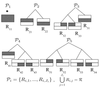
piece-wise linear models such that the IRD regressor space is di-vided into various regions. We assume that there is a lin-ear relationship between x[n] and z[n] in each region. We use a hierarchical tree structure that partitions the regressor space into various regions. We define a “partition” of the D-dimensional regressor space as a specific partitioning Pi =
{Ri,1, ..., Ri,Ji}, where SJi
j=1Ri,j = R, Ri,j is a region in
R11 R 22 R21 R32 R31 R33 R42 R43 R51 R52 R53 R54 R41 ,
Fig. 1:A full tree of depth 2 that represents all possible partitions of the two dimensional space, P = {P1, ..., PNK} and NK≈ (1.5)
2K, where K is
the depth of the tree. Here NK = 5.
the D-dimensional regressor space and R ∈ IRDis the
com-plete D-dimensional regressor space. In general, for a tree of depth K, there are as many as 1.52K possible partitions as shown in Fig. 1. Each of these doubly exponential number of partitions can be used to construct a piecewise linear model. For instance, for a jthregion Rjof partition Pi, the estimate
of y[n] is given by, ˆ
yj[n] = h(wj[t]Tx[n] + bj[t]]), (4)
where wj[t] is the weight vector in IRD, j ∈ {1, ..., Ji}, Ji
is the number of regions the feature space is divided into by the partition Pi, bj[t] ∈ IR denotes an offset, t = {n; x[n] ∈
Rj}. The overall estimate of y[n] by the partition Pi is then
given by:
ˆ
yPi[n] = h(wjx[n] + bj), (5) where j ∈ {1, ..., Ji}, x[n] ∈ Rj.
However, instead of the doubly exponential number of possible partitions, we use the context tree algorithm [6] that competes with the class of all possible partitions with a com-putational complexity only linear in the depth of the tree.
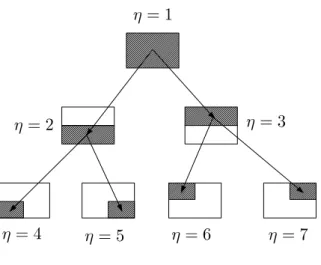
In Fig. 2, a context tree of depth K = 2, that partitions the IR2space into at most four possible regions, is shown. Here, we specifically minimize the following regret over any n [6],
n X t=1 (y[t] − ˆyq[t])2− inf Pi n X t=1 (y[t] − ˆyPi[t]) 2, (6)
where ˆyPi[t] is the estimate of y[t] by the partition Pi, i ∈ {1, ..., 1.52K
}, and ˆyq[t] is the estimate of y[t] by the context
Fig. 2:A two dimensional context tree of depth 2
In our current setting, where the feature vectors lie on a high dimensional manifold and only a subset of features are observed, we use the projections of the input vectors on the intrinsic dimension of the manifolds instead of the original feature vectors. We propose an algorithm that uses a hier-archical tree structure to track the underlying manifold and perform logistic regression on the projected IRdspace, where d is the intrinsic dimension of the manifold and d D.
3. LOGISTIC REGRESSION ON MANIFOLDS To escape the curse of dimensionality, we perform regression on high dimensional data by mapping the regressor vectors to low dimensional projections. We assume that the observed data x[n] ∈ IRDlies on time varying submanifolds Sm[n]. We
can solve the problem of non-linear regression by using piece-wise linear modeling as explained in Section 2, where the regressor space, i.e., IRD can be partitioned into several re-gions. However, in the new setting, since the data lies on sub-manifolds with lower intrinsic dimension, we use the lower dimensional projections instead of the original IRDregressor space. We define the piecewise regions in IRd for each node that correspond to the low dimensional submanifolds. How-ever, since the submanifolds are time varying, the regions are not fixed. We define these regions by the subsets [8, 9]:
<j[n] = {x[n] ∈ IRD: x[n] = Qj[n]βj[n] + cj[n],
βTj[n]Λ−1j [n]βj[n] ≤ 1, βj[n] ∈ IRd}, (7) where each subset <j[n] is a d−dimensional ellipsoid
as-signed to each node of the tree. The matrix Qj[n] ∈ IRD×dis
the subspace basis in d−dimensional hyperplane and the vec-tor cj[n] is the offset of the ellipsoid from the origin. The
matrix Λη[n] , diag{λ (1)
η [n], ..., λ(d)η [n]} with λ(1)η [n] ≥
(a) (b)
Fig. 3:(a) A parent node and its two children in an adaptive hierarchical tree. Each node (subset) is a two dimensional ellipsoid defined by its parameters {Qη[n], Λη[n], cη[n]}. (b) A dynamic hierarchical tree of depth K where
each η represents a subset defined by (7) and η ∈ {1, 2, ..., 2K+1− 1}
... ≥ λ(d)η [n] ≥ 0, contains the eigen-values of the
covari-ance matrix of the data x[n] projected onto each hyperplane. The subspace basis Qη[n] specifies the orientation or
direc-tion of the hyperplane and the eigen-values specify the spread of the data within each hyperplane [8, 9]. The projections of x[n] on the basis Qη[n] are used as new regression vectors,
βη[n] = QT
η[n](x[n] − cη[n]). We represent these regions by
a tree structure given in Fig. 3(b).
The piecewise regions are now d−dimensional ellipsoids instead of the original IRD space, therefore, we use the ap-proximate Mahalonobis distance DM [8] to measure the
closeness of the leaf nodes with the input vector x[n], i.e., η∗= arg min
η DM(x[n], <η[n]). (8)
Once the minimum distance node, η∗ is known, we then use the projection of x[n] on its subspace to calculate the new regressor vector βη∗[n]. We use this η∗ as the {K + 1}th dark node in the context tree algorithm [6] and the rest of K dark nodes are the ancestor nodes of η∗till the root node η = 1. We use each of these dark nodes to estimate z[n] as ˜
zk[n] = wk[n − 1]Tβk[n] + bk[n − 1], and linearly combine
these estimates as follows,
ˆ z[n] = K+1 X k=1 µk[n − 1]˜zk[n], (9)
where the combination weights are determined by the perfor-mance of the kthdark node in the past till n − 1 [6]. We
as-sume linear discriminants in each region and learn the weight vectors wk[n − 1] ∈ IRdand the offsets bk[n − 1] ∈ IR using
the Recursive Least Square (RLS) algorithm [3].
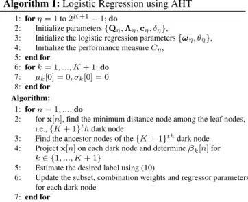
When a new data sample x[n] arrives, we first calculate the minimum distance node among the leaf nodes of the tree according to (8). We mark this node as the {K + 1}thdark node and determine the rest of the dark nodes by climbing
Algorithm 1: Logistic Regression using AHT 1: for η = 1 to 2K+1− 1; do
2: Initialize parameters {Qη, Λη, cη, δη},
3: Initialize the logistic regression parameters {ωη, θη},
4: Initialize the performance measure Cη,
5: end for 6: for k = 1, ..., K + 1; do 7: µk[0] = 0, σk[0] = 0 8: end for Algorithm: 1: for n = 1, .... do
2: for x[n], find the minimum distance node among the leaf nodes, i.e., {K + 1}th dark node
3: Find the ancestor nodes of the {K + 1}thdark node 4: Project x[n] on each dark node and determine βk[n] for
k ∈ {1, ..., K + 1}
5: Estimate the desired label using (10)
6: Update the subset, combination weights and regressor parameters for each dark node
7: end for
up the tree till the root node [?, ?]. We then project the ob-served data sample on each of these dark nodes, train a lin-ear discriminant by using the projection as the new regressor vector, and estimate the desired data label y[n] as ˜zk[n], for
k ∈ {1, ..., K + 1}. We use (9) and the logistic function in (3) to estimate the desired label, i.e.,
ˆ y[n] = h K+1 X k=1 µk[n − 1]˜zk[n] ! (10)
We next update the subsets parameters {Qk[n], Λk[n],
ck[n], δk[n]} belonging to each dark node [8, 9] using the
up-date step in the Adaptive Hierarchical Tree algorithm in [?,?]. The subset basis Qk[n] is updated using PeTReLS-FO
algo-rithm [8, 11]. We also update the combination weights µk[n]
according to the performance of the node k in estimating the desired data. Moreover, we update the logistic regressor pa-rameters by using the RLS algorithm.
4. EXPERIMENTS
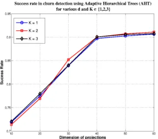
In this section, we use the proposed adaptive hierarchical trees algorithm described in Section 3 for the online churn detec-tion using high dimensional cellular network data of N = 10, 000 users. The original dimension of the regressor vec-tors x[n] is D = 164 and the desired labels y[n] ∈ {−1, 1} where y[n] = −1 for “no churn” and y[n] = 1 for “churn”. The dataset contains missing values and we observe a subset of the D features for each user. The dataset is also imbal-anced as the “no churn” class contains approximately 77% of samples. Therefore, we perform oversampling on the minor-ity class to balance the dataset [4]. We perform online logistic regression choosing d ∈ {10, 20, 30, 40, 50, 60}. We plot the success rate versus d for K ∈ {1, 2, 3} in Fig. 4.
Table 1:Success rate, false alarm rate and detection rate for AHT (d = 40, K = 3), SVM, Classification Trees and AHT-SVM
Algorithm Sucess Rate False Alarm Rate Detection Rate AHT 0.91 0.04 0.93 SVM 0.985 0.03 0.97 CTrees 0.98 0.04 0.95 AHT-SVM 0.99 0.01 0.99
The logistic regression in IRd shows great improvement in performance for churn detection in high dimensional cel-lular data for d D. In Fig. 4, we show that choosing a larger d improves the performance of the algorithm, however, it reaches saturation and further increasing d results in over-fitting and increased complexity. Hence, using only d = 40 features instead of D = 164, we achieve a success rate of over 90% with simple linear discriminant functions within each piecewise region.
It is interesting to note that for smaller K, the algorithm performs worse for d < 40, however, it reaches the same suc-cess rate as K > 2 as we choose d > 40. We also perform logistic regression on the original IRD feature vectors using online linear discriminants and the success rate is as low as 32%. Therefore, the proposed algorithm not only reduces the computational complexity but also produces outstanding suc-cess rate.
We next compare the performance of our algorithm with well known classification algorithms, i.e., SVM and classi-fication trees while using these algorithms offline. We show that our algorithm produces comparable results to batch SVM and classification trees with much less computational and time complexity as our algorithm uses linear discriminants in the online setting.
The adaptive hierarchical trees (AHT) algorithm for lo-gistic regression uses ensemble learning [4] as it linearly combines several linear discriminants and produces out-standing results with much less complexity than SVM and Classification trees (CTrees). We also use a combination of our algorithm and SVM by using SVM within each piece-wise region instead of linear discriminants (AHT-SVM) and achieved 99% success rate with a false alarm rate = 0.01. However, this approach is much complex than the original AHT and is not suitable for online learning. The results are shown in Table 1.
5. CONCLUSION
We consider the problem of logistic regression on high dimen-sional data using piecewise linear discriminants. We assume that the feature vectors lie on a high dimensional and time varying submanifolds. We propose an algorithm that effec-tively learns the underlying structure of the manifold and per-forms piecewise logistic regression on the low dimensional projections. We use hierarchical tree structure for the
piece-Fig. 4: Success rate in Churn detection using Adaptive hierarchical Trees algorithm for logistic regression with various choices of d and K
wise modeling and linear discriminants within each region. We achieve comparable results to other classification algo-rithms such as SVM and classification trees with much less complexity and memory requirement while working in an on-line setting. We use the proposed algorithm on high dimen-sional cellular data for churn detection and achieve a detection rate of 0.93 with a false alarm rate of only 0.04.
REFERENCES
[1] J. A. Deri, J. M. F. Moura, “Churn detection in large user networks ,” Intl. Conf. on Acoustics, Speech and Signal Processing (ICASSP),2014.
[2] X. Wu, X. Zhu, G.-Q. Wu, W. Ding, “Data mining with big data,” IEEE Transactions on Knowledge and Data Engineering, vol. 26, no. 1, pp. 97–107, 2014.
[3] A. H. Sayed, Fundamentals of Adaptive Filtering. NJ: John Wiley & Sons, 2003.
[4] C. M. Bishop, Pattern Recognition and Machine Learn-ing. Springer, 2006.
[5] F. M. J. Willems,“The context-tree weighting method: extensions,” IEEE Transactions on Information Theory, vol. 44, no. 2, pp. 792–798, 1998.
[6] S. S. Kozat, A. C. Singer, and G. C. Zeitler, “Univer-sal piecewise linear prediction via context trees,” IEEE Transactions on Signal Processing, vol. 55, no. 7, pp. 3730–3745, 2007.
[7] J. M. Lee, Riemannian Manifolds: An Introduction to Curvature. Springer, 1997.
[8] Y. Xie, J. Huang and R. Willett, “Change-point de-tection for high-dimensional time series with missing
data,” IEEE Journal of Selected Topics in Signal Pro-cessing,vol. 7, no. 1, pp. 12–27, 2013.
[9] Y. Xie and R. Willett, “Online logistic regression on manifolds,” IEEE Internation Conference on Acoustics, Speech and Signal Processing (ICASSP), 2013. [10] F. Khan, D. Kari, A. Karatepe and S. .S. Kozat,
“Uni-versal Nonlinear Regression on High Dimensional Data Using Adaptive Hierarchical Trees,” IEEE Transactions on Big Data, vol. PP, no. 99, pp. 1–1, 2016.
[11] F. Khan, I. Delibalta and S. .S. Kozat, “High di-mensional sequential regression on manifolds using adaptive hierarchical trees,” IEEE 25th International Workshop on Machine Learning for Signal Processing (MLSP), pp. 1–6, 2015.
[12] N. Cristianini and J. Shawe-Taylor, Support Vector Machines and Other Kernal-Based Learning Methods. Cambridge University Press, 2000.
[13] Y. Chi, Y. C. Eldar, and R. Calderbank, “PETReLS: Subspace estimation and tracking from partial observa-tions,” Int. Conf. on Acoustic, Speech, and Sig. Process-ing, March 2012.