Flowtime estimation in dynamic job shops

A THESIS

SUBMITTED TO THE DEPARTMENT OF INDUSTRIAL ENGINEERING

AND THE INSTITUTE OF ENGINEERING AND SCIENCE OF BILKENT UNIVERSITY

IN PARTIAL FULFILLMENT OF THE REQUIREMENTS FOR THE DEGREE OF

M ASTER OP SCIENCE

By

AbduUaii (^omlekgi

September, 1996

I certify that I have read this thesis and that in my opinion it is fully adequate, in scope and in quality, as a thesis for the degree of Mcuster of Science.

C . .

Assoc. Prof. İhsan Sabuncuoğlu (Advisor)

1 certify that I have read this thesis and that in my opinion it is fully adequate, in scope and in quality, as a thesis for the degree of Master of Science.

O "

Assist. Prof. Selim Aktürk

Assoc. Prof. Erdal Erel

,\pproved for the Institute of Engineering and Sciences:

^rof. Mehmet Bara

FLOWTIME ESTIMATION IN DYNAMIC JOB SHOPS

Abdullali Çömlekçi

M.S. in Industrial Engineering

Supervisor: Assoc. Prof. Ihsan Sabuncuoğiu

September, 1996

In the scheduling literature, estimation of job flowtimes has always been an important issue since the late sixties. The previous studies focus on the problem in the context of due date assignment and develop methods using aggregate information in the estimation process. In this study, we propose a new method which utilizes the job, shop and route information on an operational basis. The performance of the proposed method is measured using a simulation model. It is also compared with the existing methods for a wide variety of performance measures under various experimental conditions.

Key Words; Flowtime Estimation, Due Date Assignment, Simulation, Job Shop Scheduling

DİNAMİK İŞ ATÖLYELERİNDE AKIŞ ZAMANI TAHMİNİ

Abdullah Çömlekçi

Endüstri Mühendisliği Bölümü Yüksek Lisans

Tez Yöneticisi: Doç. Dr. İhsan Sabuncuoğiu

Eylül, 1996

Akış zamanlan tahmini, altmışlı yıllardan bu yana çizelgeleme literatüründe önemli bir konu olagelmiştir. Geçmiş çalışmalar, genellikle, teslim zamanı belir­ lenmesi kapsamında konuya eğilmişler ve bütünsel bilgiler kullanarak metodlar önermişlerdir. Bu tezde, iş, atölye ve rota bilgilerini işin operasyonları bazında ayrıştıran yeni bir akış zamanı tahmin metodu önerilmektedir. Önerilen meto­ dun performansı bir benzetim modeli ile ölçülmekte ve diğer varolan metodlarla birçok performans kriterine göre ve birçok deneysel ortamda karşılaştırılmaktadır.

Anahtar Sözcükler: Akış Zamanı Tahmini, Teslim Zamanı Belirlenmesi, Benzetim, Iş Atölyeleri Çizelgelemesi

I would like to express my gratitude to Assoc. Prof. Ihsan Sabuncuoğlu due to his supervision, suggestions, and understanding throughout the development of this thesis.

I am also indebted to Assist. Prof. Selim Aktiirk and Assoc. Prof. Erdal Erel for showing keen interest to the subject matter and accepting to read and review this thesis.

I cannot fully express my gratitude and thanks to Yasemin Ersolak and my parents for their morale support and encouragement.

I would also like to thank to Savaş Dayamk, Aynur Akkuş, Tolga Ünal, Alper Özdemir, Abdullah Daşcı, Yavuz Karapınar and Engin Topaloğlu for their friendship and support during my time in Bilkent.

My special thanks also go to my officemates in Eczacıbaşı EBI, Istanbul who supported me in any way during the last year.

1 Introduction 2 Literature Review 2.1 Introduction 3.1 Motivating P o in ts ... 17 3.2 M o d e l ... 19 3.2.1 Determination of Relevant J o b s ... 22 3.3 An Illustrative E x a m p l e ... 23 3.4 C onclusion... 25 4 Experimental Conditions 26 VI

4.1 System Considerations and Simulation M o d e l ... 26 4.2 Experimental Design 4.2.1 F actors... 27 4.3 Performance M e a s u r e s ... 30 4.4 Sensitivity Conditions ... 32 4.4.1 Macliine B r e a k d o w n ... 33

4.4.2 Processing Time V a ria tio n ... 34

4.4.3 Load V a r ia t io n ... 35

4.5 Data Collection and Computational Requirements 36 5.1 Introduction 5.2 Second Stage R e s u lts ... 42

5.2.1 Mean Absolute L a te n e s s ... 42

5.2.2 Standard Deviation of L a t e n e s s ... 61

5.2.3 Other Performance Measures ... 78

5.2.4 C o n clu sio n s... 81

5.3.1 Machine Breakdown C a s e ... 82

5.3.2 Processing Time V a ria tio n ... 84

5.3.3 Load V a r ia t io n ..., ... 106

5.3.4 C o n clu sio n s... 106

6 Conclusion 109

A Coefficients, Values and P-values of the Flowtime Estima­

tion Methods 112

5.1 Mean Absolute Lateness (M AL) versus Utilization for FCFS . . 56

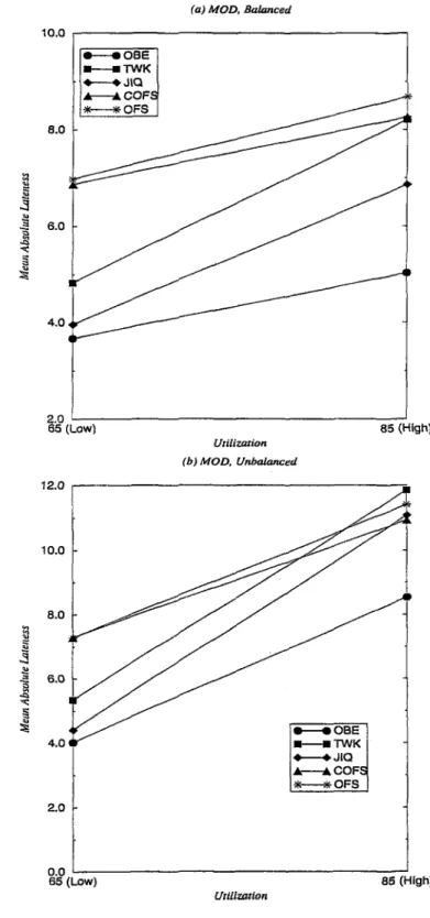
5.2 Mean Absolute Lateness (M AL) versus Utilization for MOD . . 57

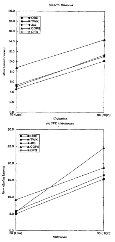
5.3 Mean Absolute Lateness (M AL) versus Utilization for SPT . . . 58

5.4 Mean Absolute Lateness (M AL) versus Balance for FCFS . . . . 59

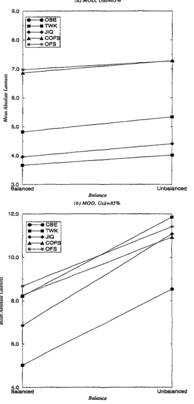
5.5 Mean Absolute Lateness (M AL) versus Balance for MOD . . . . 60

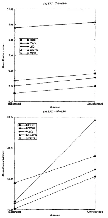
5.6 Mean Absolute Lateness (M AL) versus Balance for SPT . . . . 62

5.7 Standard Deviation of Lateness (STDL) versus Utilization for FCFS ... 71

5.8 Standard Deviation of Lateness (STDL) versus Utilization for M O D ... 72

5.9 Standard Deviation of Lateness (STDL) versus Utilization for S P T ... 73

5.10 Standard Deviation of Lateness (STDL) versus Balance for FCFS 74

5.11 Standard Deviation of Lateness (STDL) versus Balance for MOD 75

5.12 Standard Deviation of Lateness (STDL) versus Balance for SPT 76

5.13 Meaxi Absolute Lateness (MAL) versus Efficiency Levels for Bal­ anced Shop ... 92

5.14 Standard Deviation of Lateness (STDL) versus Efficiency Levels for Balanced S h op ... 93

5.15 Mean Absolute Lateness (MAL) versus Efficiency Levels for Un­ balanced S h o p ... 94

5.16 Standard Deviation of Lateness (STDL) versus Efficiency Levels for Unbalanced S h o p ... 95

5.17 Mean Absolute Lateness (MAL) versus Processing Time Varia­ tion ( P V ) ... 102

5.18 Standard Deviation of Lateness (STDL) versus Processing Time Variation (PV ) ... 103

0.1 Performance Results for Balanced Shop Under Low Utilization (65%) L e v e l ... 44

0.2 Performance Results for Unbalanced Shop Under Low Utiliza­ tion (65%) Level ... 45

5.3 Performance Results for Balanced Shop Under High Utilization (85%) L e v e l ... 46

0.4 Performance Results for Unbalanced Shop Under High Utiliza­

tion (85%) Level 47

5.5 Analysis of Variance for Mean Absolute Lateness ... 50

5.6 Analysis of Variance for Mean Absolute Lateness Under Low Utilization (65%) Level ... 51

5.7 Analysis of Variance for Mean Absolute Lateness Under High Utilization (85%) Level ... 52

5.8 Analysis of Variance for Mean Absolute Lateness for Balanced S h o p ... 53

5.9 Analysis of Variance for Mean Absolute Lateness for Unbalanced S h o p ... 54

5.10 Duncan’s Multiple Range Tests for M A L ... 64

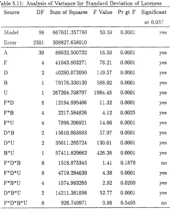
5J1 Analysis of Variance for Standard Deviation of Lateness . 65

5.12 Analysis of Variance for Standard Deviation of Lateness Under Low Utilization (65%) L e v e l ... 66

5.13 Analysis of Variance for Standard Deviation of Lateness Under High Utilization (85%) Level ... 67

5.14 Analysis of Variance for Standard Deviation of Lateness for Bal­ anced Shop ... 68

5.15 Analysis of Variance for Standard Deviation of Lateness for Un­ balanced Shop ... 69

5.16 Duncan’s Multiple Range Tests for STDL I I

5.17 Best Flowtime Estimation Methods for ML ... 78

5.18 Duncan’s Multiple Range Tests for Other Performance Measures 80

5.19 Performance Results for Machine Breakdown Under High Uti­ lization (85%) Level ... 85

5.20 Machine Breakdown Results for FCFS/Low Utilization (65% )/Bal-anced S h o p ... 86

5.21 Vlachine Breakdown Results for FCFS/Low Utilization (65%)/Un-balanced S h o p ... 87

5.22 Machine Breakdown Results for M O D /Low Utilization (65% )/Bal-anced S h o p ... 88

5.23 Machine Breakdown Results for M O D /Low Utilization (65%)/U n-balanced S h o p ... 89

5.24 Machine Breakdown Results for SPT/Low Utilization (65% )/Bal-anced Shop ... 90

5.25 Machine Breakdown Results for SPT/Low Utilization (65%)/U n ­ balanced S h o p ... 91

5.26 Processing Time Variation Results for FCFS / High Utilization (85%)/Balanced S h op ... 96

5.27 Processing Time Variation Results for FCFS / High Utilization (85%)/Unbalanced S h o p ... 97

5.28 Processing Time Variation Results for MOD / High Utilization (85%)/Balanced S h o p ... 98

5.29 Processing Time Variation Results for MOD / High Utilization (85%)/Unbalanced S h o p ... 99

5.30 Processing Time Variation Results for SPT / High Utilization (85%)/Balanced S h op ...100

5.31 Processing Time Variation Results for SPT / High Utilization (85%)/Unbalanced S h o p ... 101

5.32 Load Variation Results for FCFS / Low Utilization (65%) . . . 104

5.33 Load Variation Results for MOD / Low Utilization (65%) . . . . 105

5.34 Load Variation Results for SPT / Low Utilization (65%) . . . . 107

A .l Coefficients, p-values and values for OBE/FCFS/Unbalanced

Shop/High U t iliz a t io n ... 113

A .2 Coefficients, p-values and values for OBE/FCFS/Unbalanced

Shop/Low U tilization...114

A.3 Coefficients, p-values and values for OBE/FCFS/Balanced Shop/High U t iliz a t io n ... 115

A .5 Coefficients, p-values and values for OBE/M OD/U nbalanced Shop/High. Utilization/Iteration # 1 ... 116

A .6 Coefficients, p-values and R^ values for OBE/M OD/U nbalanced Shop/High Utilization/Iteration # 2 ... 117

A .7 Coefficients, p-values and R^ values for OBE/M OD/Unbalanced Shop/High Utilization/Iteration # 3 ... 118

A .8 Coefficients, p-values and values for OBE/M OD/U nbalanced Shop/High Utilization/Iteration # 4 ... 119

A .9 Coefficients, p-values and R^ values for OBE/M OD/Unbalanced Shop/High Utilization/Iteration ^ 5... 120 A .10 Coefficients, p-values and R? values for OBE/M OD/Unbalanced

Shop/High Utilization/Iteration # 6 ... 121

A .11 Coefficients, p-values and R^ values for OBE/M OD/U nbalanced Shop/Low Utilization/Iteration # 1 ... 122

A. 12 Coefficients, p-values and R^ values for OBE/M OD/U nbalanced Shop/Low Utilization/Iteration ^ 2 ... 123 A. 13 Coefficients, p-values and R^ values for OBE/M OD/U nbalanced

Shop/Low Utilization/Iteration ... 124

A .14 Coefficients, p-values and R^ values for OBE/M OD/U nbalanced Shop/Low Utilization/Iteration ^ 4 ... 125 A .4 Coefficients, p-values and values for OBE/FCFS/Balanced

Shop/Low U tilization...115

A. 15 Coefficients, p-values and R^ values for OBE/M OD/U nbalanced Shop/Low Utilization/Iteration # 5 ... 126

A .17 Coefficients, p-values and B? values for OBE /M O D /B alanced Shop/High Utilization/Iteration # 1 ... 128

A .18 Coefficients, p-values and B? values for OBE /M O D /B alanced Shop/Low Utilization/Iteration # 1 ... 128

A. 19 Coefficients, p-values and B? values for OBE /M O D /B alanced Sfiop/High Utilization/Iteration ^ 2 ... 129

A .20 Coefficients, p-values and B? values for O B E /M O D /B alanced Shop/Low Utilization/Iteration ... 129

A .21 Coefficients, p-values and B? values for O BE/M O D /Balanced Sfiop/High Utilization/Iteration # 3 ... 130

A .22 Coefficients, p-values and B? values for OBE/M O D/Balanced Shop/Low Utilization/Iteration ^ 3 ... 130

A .23 Coefficients, p-values and B? values for O BE/M O D /Balanced Shop/High Utilization/Iteration ... 131

A .24 Coefficients, p-values and B? values for O BE/M O D /Balanced Shop/Low Utilization/Iteration # 4 ... 131

A .25 Coefficients, p-values and B?' values for OBE /M O D /B alanced Shop/High Utilization/Iteration # 5 ... 132

A .26 Coefficients, p-values and B? values for O B E /M O D /B alanced Shop/Low Utilization/Iteration # 5 ... 132 A .16 Coeificients, p-values and B? values for OBE/M OD/Unbalanced

Shop/Low Utilization/Iteration # 6 ... 127

A .27 Coefficients, p-values and B^ values for OBE /M O D /B alanced Shop/High Utilization/Iteration # 6 ... . . . . 133

A .29 Coefficients, p-values and values for OBE/SPT/Unbalanced

Shop/High U t iliz a t io n ... 134

A .30 Coefficients, p-values and values for OBE/SPT/Unbalanced

Shop/Low U tilization... 135

A .31 Coefficients, p-values and R? values for O BE/SPT/Balanced Shop/High U t iliz a t io n ... 136

A .32 Coefficients, p-values and R^ values for OBE /SPT/Balanced Shop/Low U tilization... 136

A .33 Coefficients, p-values and R } values for COFS/Unbalanced Shop/High U tiliza tion ...137

A .34 Coefficients, p-values and R? values for COFS/Balanced Shop/High U tiliza tion ...137

A .35 Coefficients, p-values and R? values for COFS/Unbalanced Shop/Low U tiliza tion ...138

A .36 Coefficients, p-values and FF values for COFS/Balanced Shop/Low U tilization ...138

A .37 Coefficients, p-values and IF· values for OFS/Unbalanced Shop/High Utilization ... 139

A .38 Coefficients, p-values and R^ values for OFS/Balanced Shop/High U tiliza tion ...139 A .28 Coefficients, p-values and values for O BE/M O D /Balanced

Shop/Low Utilization/Iteration # 6 ... 133

A .39 Coefficients, p-values and R^ values for OFS/Unbalanced Shop/Low U tiliza tion ... 140

A.41 Coefficients, p-values and B? values for JIQ and T W K Unbal­

anced Sfiop/Higli U tilization...141

A .42 Coefficients, p-values and values for JIQ and T W K Balanced Shop/High U tiliz a t io n ... 141

A.43 Coefficients, p-values and R^ values for JIQ and T W K Unbal­ anced Shop/Low U tiliz a tio n ... 142

A .44 Coefficients, p-values and R^ values for JIQ and T W K Balanced Shop/Low U tilization...142

A.40 Coefficieiits, p-values and. values for OFS/Balanced Shop/Low U tiliza tion ...140

C .l Analysis of Variance for Mean Lateness ... 154

C.2 Analysis of Variance for Mean T a x d in e s s ... 155

C.3 Analysis of Variance for Mean Squared Lateness ... 156

C.4 Analysis of Variance for Mean Semi-Quadratic Lateness . 157 C.5 Analysis of Variance for Mean F l o w t i m e ...158

Introduction

In the job shop scheduling literature, estimation of job flowtimes has always been an important issue since the late sixties. However, the problem has been identified mostly within the context of due date assignment. This is due to the fact that flowtime estimation is critically important when assigning due dates to be promised to the customers. Beyond the objective of due date assignment, quality of flowtime estimates also leads to significant improvements in the shop floor control activities, such as order review/release, evaluation of the shop performances, identification of jobs that require expediting, etc.

The research problem studied in this thesis is the estimation of the time spent by the jobs in the system from their arrival until the completion of all its processing activities. The difficulty of the problem comes from the dynamic and stochastic nature of the job shop environments (i.e. arrival of hot jobs, sudden machine breakdowns and variations in machining conditions, etc.)

The studies in the Uterature approach to the problem by identifying the key information sources required in flowtime estimation. As a result, job, shop and route information are outlined as the major elements in the developed estimation methods. Among them, route is reported and used cls the most valuable information source.

In the previous studies, researchers use the above information sources in aggregate terms and thus ignore the benefits of using the detailed shop and route congestion information for flowtime estimation.

In this study, we develop a new method which estimates operational flow- times in dynamic job shop environments. The proposed method utilizes job, shop and route information and exploits these information on the operational basis. The machine imbalance and dispatching rule information are also con­ sidered.

The rest of this thesis is organized as follows. In Chapter 2, we present the literature for both the analytical and the simulation approaches. In Chapter 3, basic structure and characteristics of the proposed flowtime estimation method are described. The key components of the model are reviewed via an illustrative example. In Chapter 4, we define the experimental design and the details of our simulation model. In Chapter 5, the results of the simulation experiments are discussed with the applications of appropriate statistical procedures. Finally, the concluding remarks are made and further research directions are outlined in Chapter 6.

Literature Review

2.1

Introduction

Due date assignment is one of the main application areas of flowtime estima­ tion. As it is frequently observed in the literature, most of the research efforts directed to the flowtime estimation take place within the context of due date assignment (Eilon and Hodgson [11], Eilon and Chowdhury [10], Taylor and Moore [31]). This evolves from the fact that due date setting procedures re­ quire flowtime estimation methods as a support tool. In this chapter, we will discuss the due date assignment literature to the extent that flowtime estima­ tion efforts exist for dyneimic systems. This means that we will not discuss the studies conducted for static systems nor the studies that calculates due dates for dynamic systems based on predetermined tightness factors.

The literature on flowtime estimation is comprised of mainly two approaches : analytical approach and simulation approach. Cheng and Gupta [8] provides an extensive survey of both approaches in due date assignment. He also gives a framework for scheduling problems consisting of the due date determination process.

the development of sophisticated analytical models. Consequently, restrictive assumptions are made in order to obtain some feasible solutions. But these assumptions prevent the application of analytical models in real life situations. Thus, in many cases, simulation seems to be the sole feasible way of handling such complex systems in flowtime estimation. However, simulation approach may not always lead to reliable estimates. Moreover, in striving for the accu­ rate and precise estimates, a great number of computer runs may be required. In conclusion, there is a trade-off between the analytical and simulation ap­ proaches which in turn leads to the development of literature in both directions. As our primary concern is on simulation approach we will mainly focus on the simulation side of the literature.

In the rest of this chapter, we will first briefly summarize the analytical studies and then discuss the research works which are primarily based on sim­ ulation approach.

2.2

Analytical Approach

Flowtime estimation can be also seen as a key component of scheduling systems. In such a study, Miyazahi [21] proposes a scheduling system to reduce job tardiness by combining a due date assignment procedure with a sequencing procedure. He derives formulae to obtain the mean and the standard deviation of job flowtimes. Number of machines, ratio of the load to the production capacity and the machine utilization information are used in estimating mean and the standard deviation of flowtimes. W ith the help of the formulae and an adjustment factor, due dates are assigned to the jobs. The new combined approach performs better than the conventional scheduling systems. However, the performance of the proposed flowtime estimation method is not measured separately.

exactly, his second formula approximates the standaxd deviation. Cheng [3] ex­ tends Miyazaki’s work and derives both the mean and the standard deviation of the job flowtimes exactly by using Laplace transforms method. The robustness of results to the violation of the assumption of equality of the mean processing times of the machines in the shop is also examined and it is found to be robust.

Enns [12] extends the works of Miyazaki [21] and Cheng [3] and proposes four analytical flowtime assignment methods each using combinations of job and shop information. He compares these methods with respect to many per­ formance criteria and reaches the conclusion that both shop and job informa­ tion are useful in estimating flowtimes. Another important finding of this study is that as the accuracy and precision of the estimates improve, the lateness dis­ tribution becomes to be normally distributed. However, the proposed methods are only valid when the dispatching rule is first-come-first-served (FCFS).

Cheng [4] presents another analytical model that can determine the opti­ mal coefficients for T W K (Total Work Content) and TW K-N OP (Total Work Content and Number of Operations) rules (see Section 2.3 for the definitions of these rules). However, the proposed model is based on some restrictive as­ sumptions on queue discipline and processing time distribution. The analytical results are compared with the simulation results and validated through the ob­ servations that the results agree with each other. Cheng [4] also claims that TW K-N O P is more effective in minimizing missed due dates costs in a job shop. Cheng [7] elaborates more on the determination of coefficients for TW K for an assembly shop. A critical path based analysis of the job processes in­ formation is developed to obtain the coefficient value for T W K that minimizes the expected value of the squared lateness. A formula which approximates the optimal coefficient value is derived and it is shown that the approximation er­ ror is below 30 per cent in the worst case situation. It is also shown that that the proposed method is effective for jobs with varying structural complexities.

Cheng [5] proposes another method of assigning optimal due dates and a heuristic approach which minimize the average amount of missed due dates in a single machine shop with the queue discipline of SPT. He evaluates the

analytical results by comparing with the simulation results for various shop conditions and concludes that the heuristic method can produce accurate due dates eifectively.

Shanthikumar and Buzacott [28], [29] model a dynamic job shop as the open queuing network and derives approximations to the mean and the standard deviation of flowtimes. However, their model produces effective approximations only for the job shops with local dispatching rules. Buzacott and Shanthikumar [2] show that the mean and standard deviation of the flowtimes are smaller for SPT when compared with the FCFS dispatching rule. Shanthikumar and Sumita [30] extend this study and develop approximations to the distribution of the flowtimes. They also use these distributions in controlling the total costs incurred for tardiness and earliness of the jobs while assigning due dates.

Finally, Lawrence [20] proposes a due setting methodology for which the flowtime error distributions are approximated empirically by Ramberg-Schmeiser [26] distributions. Using the properties of Ramberg-Schmeiser distributions, the best due dates are obtained for different objectives such as minimizing mean squared lateness, minimizing total tardiness and eaxliness costs and at­ tainment of some service level targets.

2.3

Simulation Approach

One of the early works in the simulation approach has been conducted by Conway [9]. In this study, four flowtime estimation methods are compared: Total Work Content (T W K ), Number of Operations (N OP), Constant (CON), Random (RDM ). The mathematical definitions of these methods are as follows :

T W K : Fi = kPi NOP: Fi = kNi CON: Fi = K RDM: Fi = kXi where, Fi Pi Ni Xi k j <

Flowtime estimate of job i

Total processing time of job i

Number of operations of job i

A random number assigned for job i

constants

These methods are used in assigning the due dates. The results of his simulation experiments indicates that the methods which utilizes the job in­ formation perform better than the ones that do not consider. Conway [9] also reports that there exists a relationship between the due date assignment methods and the dispatching rules.

Eilon and Hodgson [11] compare the performances of dispatching rules when due dates are cissigned by T W K method. It appears that SPT is the best dispatching rule with respect to several performance measures such as waiting times, queue lengths, etc. In this study, the best ki values which minimizes the total penalty costs for earliness or tardiness are also obtained. This study is also the first simulation study which aims at finding the best coefficient values.

Eilon and Chowdhury [10] first uses shop congestion information in estimat­ ing flowtimes. In this study, T W K is compared with three new methods which are all extensions of T W K : Jobs in Queue (JIQ ), Delay in Queue (DIQ), M od­ ified Total Work Content (M T W K ). The mathematical forms of these methods are :

D IQ: Fi = hPi + h W JIQ: Fi — k\Pi -)- k2Qi M T W K : Fi = hPt^

where,

W = Mean waiting time per job.

Qi = Number of jobs in progress along the route of job i. ki,k2 = constants

Results indicate that JIQ method, which employs the shop congestion in­ formation, outperforms all other methods. JIQ also produces better results than the other methods for a shop with fluctuating load ratio. This is because, the other methods do not make use of the shop load information. Another observation of this study is that due date dependent dispatching rules pro­ vide better results in terms of missed due dates as compared to the due date independent dispatching rules.

Weeks [34] proposes a method which also combines job and shop informa­ tion;

Fi = max{Pi + W + I{TQi)crw, Pi)

where,

T Q i= Total number of jobs in the system when job i arrives.

I{T Q i)=

1 if TQi < TQ — (ttq

0 if TQi — (Ttq < TQi < TQ + arq

- 1 i î T Q i > T Q + (ttq

T Q = Mean number of jobs in the system.

cTw= Standard deviation of waiting times of jobs.

This metbod is found to be superior over the previously proposed methods for the performance measures such as mean lateness, mean earliness, and mean missed due dates. Three diiferent types of production systems are also investi­ gated in the study and it is empirically shown that, as the structural complexity of the shop is increased, the performances of the methods are negatively af­ fected. It is also reported that the performances are not much influenced from the shop size. It is noted that shop size is being characterized by the number of machines and workcenters in the shop whereas the shop complexity is char­ acterized only by the increased structural departmentation (divisions in the shop).

Taylor and Moore [31] demonstrate the use of network modeling and simu­ lation in estimating job flowtimes for a job shop. They present their approach via an example and show how a job shop can be modeled as a network with the Q-GERT technique. They also emphasize that the practical benefits that may be achieved by network modeling.

Bertrand [1] proposes a new method of flowtime estimation which exploits time-phased workload information of the shop :

Fi = Pi + P x S L x N i + Fi{Wt)

where.

P SL FiiW,)

Mean processing time in the shop

Minimum allowance for waiting

Additional flow time allowance, dependent in observed congestion due to the workload, Wj, in the shop

Two factors are used in analyzing the performance of the method: SL and

CLL (capacity loading limit). The method is compared with its version that does not take into account the time-phcLsed workload information (i.e. Fi{Wt)

is omitted from the model). It is seen that time-phased workload and capacity information significantly decreases variance of the lateness.

Ragatz and Mabert [25] give an extensive comparison of eight different methods and evaluate their performances for a hypothetical job shop with re­ spect to three performance measures: mean tardiness, mean absolute lateness and standard deviation of lateness. T W K , NOP, TW K-NOP, JIQ, WIQ (sim­ ilar to JIQ except that the total processing times of jobs on the route is used instead of the number of them), W EEK’s method, JIS (similar to JIQ except that the number of jobs at the system is used instead of the number of jobs on the route), and RM R (Response Mapping Rule) are compared with this study.

R M R is the proposed method in the study, and it utilizes the response surface mapping procedures to identify the significant factors in estimation of the flowtimes. Three different models are constructed for each dispatching rule used in the analysis. This is needed because different factors appear to be significant for each dispatching rule.

An interesting result of this study is the poor performance of W EEK’ s method with respect to most of the other flowtime estimation methods. It is also reconfirmed by this study that both shop and job information are useful in flowtime estimation. Another observation of the study is that the workload information along the route is more useful than the general shop information. It is also reported that the use of more detailed information with R M R does not improve the performance much over the other methods that use more aggregate information.

Cheng [6] exploits a hypothetical job shop to determine the main and in­ teraction effects o f: due date assignment method, dispatching rule, and shop load ratio. He employs multiple regression analysis on the results to estimate the mathematical relations between these three factors and the performance measure of percentage late jobs. The derived regression model is used to obtain percentage of late jobs for any given shop conditions characterized by the three factors.

Kanet and Ckristy [17] compare T W K with the Processing Plus Wait­ ing (P P W ) method for a general job shop with forbidden early shipment of completed jobs. PPW method estimates a jo b ’s flow allowance by adding an estimate of the waiting time, which is proportional with the number of opera­ tions, to the total processing time of a job. The experimental results showed that T W K is superior to PPW in terms of the performance measures of mean tardiness, proportion of tardy jobs, and mean inventory levels.

Fry, Philipoom and Markland [15] investigate the job and shop characteris­ tics which affect a jo b ’s flowtime in a multistage job shop. The characteristics they have identified are ;

a) Job Factors

— Sum of all operation times in the BOM.

— Sum of ail operation times on the critical path of the BOM — Total number of assembly points in the BOM

— Number of branches or components in the BOM

b) Shop Factor

— Total amount of work in the system

W ith these factors, they construct two linear and two multiplicative nonlin­ ear models and estimate the coefficients of the factors via regression analysis. The following conclusions are drawn from this study:

a) Models using product structure and shop conditions can estimate flow- times better than the others.

b) Linear models are superior to the multiplicative models.

Vig and Dooley [32] propose two new flowtime estimation methods which utilize flowtime per operation information of the recently finished jo b s : Op­ eration Flowtime Sampling (OFS) and Congestion and Operation Flowtime Sampling (OOFS). The mathematical forms of these methods are:

OFS: COES:

where,

Fi — kiT -|- k2Ni -t- k^Pi

Fi

k iT

k2Qi

k^Ni

k^Pi

Ti = A x Ni

= Ai/NRi + A2/NR2 + A3/NR3

Ai, A2, A 3 = Flowtimes of the three most recently completed jobs

N Ri, N R2, NR3 = Number of operations of the three most recently completed jobs

These methods are compared with JIQ and TW K-N OP methods under various shop conditions. The results show that COFS and JIQ methods give the overall best performances, but OFS method shows also good performance when MOD dispatching rule is used. The interactions of the experimental factors are also analyzed through analysis of variance. It is observed that flowtime estimation method, dispatching rule, and shop balance all influences the performance of the shop for all performance measures. Vig and Dooley [33] extend this work by combining static and dynamic estimates to obtain job flowtime estimates with the following method :

Fi = {1 — a)Fst + oiFdi

n VVcigliliiig faclor

= Static flowtime estimate (mean flowtime)

l'\li = Dynamic flowtime estimate of job i

hi this method, the dynamic estimates are produced by COFS and 01'\S methods. Witli the data collected from steady state simulation runs, the actual and dynamic ilowtime estimates are compared one by one and a range for I Ik' wi'ighting factor o- is obtained. The o- value to be implemented is si'lected from this range.

Vig and Dooley [32] and [33] also investigate the effect of the shop balance on the performance of the flowtime methods and they conclude that the balance information siguiflcantly affects the iierformance of the flowtime estimation methods.

(îee and Smith [16] propose an iterative procedure for estimating ilowtinu's when due date dependent dispatching rules are used. Two flowtime estima­ tion methods irsing local (job related) information and global (both job and shop ndated) information are also employed to present the benefits of iterativi' estimation.

Local Method:

Fi = kiPi + k2lV^ + hP^ + k,Nf

(llohal Method:

Fi

=

+

+

+

+

Ri = Total processing time for operations in queue along the routing of job i

Si — Total processing time for operations elsewhere in the shop that require machines that are required by job i

It is reported that the global rule gives better estimation performance most of the time. It is interesting to note that the load information out of the route,

{Si), is valuable in estimation of the flowtimes.

The impact of the iterative approach is demonstrated also by comparing the second method with the RM R approach previously proposed by Ragatz and Mabert [25]. The experimental results show that using the iterative approach for due date dependent dispatching rules improves the performance of the flow­ time estimation methods. This is because, the regression equations fitted for a method, change at each iteration. Since due dates are based on the flowtime estimates, the dispatching in the shop is also changed at each iteration.

Enns [13], [14] describes a dynamic estimation method which employs a dynamic version of the PPW method. By using exponentiedly smoothed flow­ time estimation error feedback, the operation lateness variance is estimated and used when setting due dates for jobs. It is shown in this study that the estimation errors are normally distributed. By making use of this observation, they describe a method of setting due dates that enables the achievement of the desired percentage of tardy jobs so that the delivery performance is con­ trolled. It is also reported that the due date dependent dispatching rules lead to better performance as compared to due date independent rules.

Kaplan and Unal [18] suggest a cost based approach for determining the due dates. The proposed approach states that the due dates are calculated by summing the flowtime estimate with a multiple of the estimated standard deviation of the flowtime estimation error. Their analysis is composed of two stages. In the first stage, a flowtime estimation model is derived. By performing a correlation analysis over the shop, job and route related factors, the key factors affecting the shop are determined. Several models are developed for

(vu li coml)inat,ion of these factors and one of the models is selected to be used in tlie due date assignment procedure. In the second stage, the coefficient to he used when adding a multiple of the standard deviation of estimation error, is sought. 'I'his coefTicient is obtained by optimizing the total cost (liolding cost plus tardiness cost) function. 'I'liey also consider the balance of the shop in their e.xperimental study.

In the literature, api3İying multiple regression to the data collected \ ia simulation experiments is a commonly used procedure for ilowtime estimation. Philipoom, Re('s and Wiegmann [21] present the use of neural networks a.s a.ii alt('rna.tive to (his approach. In tlu'ir study, (hey estimate the coedicients of ( he methods previously tested by llagatz and Mabert [25] with neural networks instead of mull,iple regression. It is observed that the neural network approacli oid.pcnforms the conventional regression based approach in two of the threM' shops tested in their study.

The interactions between the ilowtime estimation methods and the dis­ patching rules are significant. Hence, the dispatching rule used in a system influences both the shop performance and the performance of i.lu' flowtime estimation method ([6], [8], [9], [11], [12], [21], [25]).

• Both shop and job characteristics are important for estimation of flow- times ([1]. [3], [10], [12], [21], [25], [.32], [3-3], [34]).

• Splitting the shop congestion information as the load on the route and the load out of the route enhances predictive power of the flowtime estimation methods. Especially, the load information along the route of a job is secui to be more, useful than the other general shop information ([10], [25], [32], (3.31).

• Due date dependent dispatching rules provide superior shop performance over the due date independent rules ([10], [14]).

• Shop balance information significantly affects the performance of the flowtime estimation methods ([IS], [32], [33]).

• Use of aggregate information leads to almost the same performance when compared with the use of more detailed information with RM R ([25]).

In the rest of this thesis, we will evaluate the problem of estimation of flowtimes by taking into account these observations and will propose a new

-Proposed Method

In this chapter, we describe the basic structure and characteristics of the pro­ posed flowtime estimation method.

3.1

Motivating Points

In this section, we outline the main ideas which motivated us to develop a new flowtime estimation model.

1) Previous research indicated that total load on the process route of an arriving job provides valuable information in flowtime estimation. (Eilon and Chowdhury [10], Bertrand [1], Ragatz and Mabert [25], Vig and Dooley [32], [33]) Moreover, we expect that distribution of this load on the machines along the route of the job is also as important as the total load itself. As one can intuitively expect, the existing load of the machine close to the beginning of the route of the job would affect the flowtime of that job more than the load close to the end of the route. Because state of the system could be quite different when the job arrives at the machines for later operations. Thus, splitting the route information with respect to operations of the job can improve the performance of a flowtime

estimation method.

2) Previous research has also indicated that consideration of total loads of the jobs elsewhere in the shop (i.e. the jobs which are not currently at the respective machines on the route of the arriving job, but will visit these machines later in their processes) is also important (Gee and Smith [16]). Because these jobs will eventually bring additional loads to the route of the arriving job. Hence, both timing and distribution of these so called “other jobs” should also be considered in flowtime estimations.

3) Many researchers have demonstrated that dispatching rules used to se­ quence jobs also affect the performance of estimation methods ([6], [8], [9], [11], [12], [21], [25]). For example, Ragatz and Mabert [25] investi­ gated this situation and proposed different flowtime estimation models for different dispatching rules in their proposed ’’ Response Mapping Rule

(R M R )” .

In our study, we also use different dispatching rules for flowtime estima­ tion. But the use of dispatching rule information in our case is quite different than the usage in the literature; instead of using a separate prediction model for each rule, we use the same model but redefine the variables for each dispatching rule. For example, when total load is used as a variable in the model, the total operation times of all the jobs in the queue is calculated for FCFS rule whereas the total operation time of the jobs with smaller operation times than the arriving job is used for the SPT rule. Thus, meanings of the variables in our model are quite different for different dispatching rules.

4) It has been also shown in the literature that the performance of the flowtime estimation methods are significantly affected as the balance of the shop deteriorates. Bertrand [1] uses the time-phased profile of the workload information and implicitly considers the shop balance in his proposed model. However, there is currently no study in the literature which explicitly considers machine imbalance information in flowtime es­ timation. In our study, however, we will consider explicitly the long run load information for each machine.

3.2

Model

In this section, we describe the basic characteristics and structure of the pro­ posed flowtime estimation model whose motivating points are outlined in the previous section. In the model, the following variables are considered:

a) the processing time of the job,

b) the existing total load o f the machine on which the job will be processed, and

c) the total load that will soon arrive to the machine on which the job will be processed.

These variables have been selected because they capture most of the oper­ ational information of a job. The generic model is as follows :

: Sum of processing times of the relevant jobs^ at the queue of machine

j that job i will have its kth. operation

X^ji '■ Sum of processing times (on the machine j that job i will have its kth.

operation) of the relevant jobs^ at the queues of the machines other than machine j but require machine j in the future

X^·^: Processing time of job i at machine j for its kth operation

’•Only a subset o f jobs are used in calculating the values o f the variables. These jobs are called the relevant jobs. The criteria for selecting these relevant jobs are given in section 3.2.1.

c’ij,C2j,c^j : coefficients

When job i arrives to the system, the PFji values are calculated for each operation by using the above equations. Then, the total flowtime estimate Fi

is obtained by summing these values.

In the balanced shop case, since the utilizations of the machines are nearly the same, they can be ti’eated as identical machines. Thus, the above model is simplified in to:

P F t = cfX fi + + 4 x 1 , (1.2) where,

PF^ : Partial flowtime of job i for its kth operation

X^·: Sum of processing times of the relevant jobs at the queue of the machine that job i will have its ¿th operation

X21 : Sum of processing times of the relevant jobs at the queues of the ma­ chines other than the machine that job i will have its A;th operation, but will require that machine in the future

X з¿; Processing time of job i for its fcth operation c^,C2,C3 : coefficients

The following equations are obtained for a job shop comprised of 5 ma­ chines : a) Unbalanced shop : Machine PFl, = c\,X\,, + c\,Xh,i PF\i ~ PFh = ct.xtu + PF!i = 4 , x i u + 4 A Machine # 2 + 4l^3U I X’'2 + 1 .3 y3 + ^31-^318 + 4 A P F l = cloA'i 4- chnXi jj ^2 _ 2 v2 I 2 A"? ^^ 2i — ' ^22‘‘^22z P Fii — ^12^121 PF.% = C A i P F l = c f A i Machine # 3 ^22'^'222 X ^22^222

“I" C ooA o*),*

PFk = cl3^Ti3, + <^23-'^23i n c ’’’ 2 v2 I 2 v2 ^ -^38 ~ '^13"^138 + C23A23j P Fii — ‘^ ? 3 '^ 1 3 i + ^23X23« P F i, = cUXfai + c | 3 ^ l 3 8 P Fii = c h X L ·_'13^138 + ^23-^238 Machine # 4 PFli = c \ A i_14^14i PFl = cl A + 441^248 + C24^248 PFi = cl A + 4 A PFti = c t A + 44^248 + €24X248 '1 4 ^ '· 148 P F l = c \ A Machine # 5 PFii = €45X45^ PFi, = chX + 4 2 -^ 3 2 8 -> y 9 ■ t" ^3 2 ^ 3 2 8 - L . ^ ^ + C 32X 328 + 4 2 X 3 2 8 4 - U Y '· w ‘'33^'-338 + 4 3 X I 3 8 + 4 3 X 3 3 8 + 4 3 X 3 3 8 + 4 3 X 3 3 8 + 4 4 X 3 4 8 + O I A + 4 4- ^348· + 4 4 X 3 4 8 + <^34X348 15^'· 158+ 4,,X:' PFi, = c l A PFi, = c t A P F l = cl A_15^'-158 + 4 5 "^ 2 5 8 + 4 5 -^ 3 5 8 I „ 2 v 2 + C зgA з5¿ + 45X351 + 4s-^358 + 4sX|58 25^258 + 45-^258 + 4s-^258 + 45'^f58

b) Balanced shop : PFl = clx}, + 4x^, + 4 x i, PF? = c i x i + 4 x i + 4 x i P F f = c ? x f, + c?At· + ciA t- P F t = c\Xt^ + c|A|, + c|A|, P F ! = 4 x ! i + 4 x 1 , + c|a _:3i

3.2.1

Determination of Relevant Jobs

In the proposed nnethod, while calculating the values of X n j and X2ij for an arriving job i, we do not consider all the jobs in the queues. Instead we focus on some subset of the jobs, and eliminate the rest by using a selection criteria. The jobs that are selected are called “relevant” jobs whereas the others are simply called “irrelevant” . Since different sets of jobs are used when calculating the values of Xuj and X2ij·, we use different criteria in determining the relevant jobs for each variable.

Determination of Relevant Jobs for

X\ji:

The jobs residing at the queue of machine j (the machine on which the arriving job will be processed) are evaluated by the following criteria for each dispatching rule.

FCFS: All of the jobs are selected as “relevant” .

SPT·. The jobs which have smaller operation times than the arriving job are selected as “relevant” .

MOD: Let k be the index for a job waiting at the queue of the machine j

and let i be the index for the arriving job.

if its priority index is lower than the job z’s index.

The priority index for job k, is assigned just as the modified operation due date (see section 4.2.1), whereas the priority index of job i is assigned as the ready time plus a fraction of its total flow allowance. This fraction is calculated by dividing the total processing time required until job i finishes its operation on machine j , by the total processing time required for all of its operations.

Determination of the Relevant Jobs for

X-

2ji’.

The jobs residing at the queues of machines other than machine j are eval­ uated by the following criteria for each dispatching rule.

FCFS: All of the jobs are selected as ‘‘relevant” .

SPT : The jobs which have smaller operation times than the arriving job are selected as “relevant” .

MOD: Let k be the index for a job residing at the queue of a machine other than machine j , and i be the index for the arriving job.

We again calculate two priority indices for each job and select job k as “relevant” if its priority index is lower than that of job i.

The priority index for job i is calculated in the same way as it was calculated for X\ji. The priority index for job k is assigned as a fraction of its remaining flow allowance where this fraction is calculated by dividing the total processing time required until job k finishes its operation on machine j , by the remaining total processing time.

3,3

An Illustrative Example

In this section, we will try to explain the proposed method in more detail via an example.

Let us suppose that job i has just arrived at an unbalanced shop with 5 machines. Assume that this job will visit machine # 5 , machine # 3 and machine # 2, for its first, second and third operations, respectively.

The proposed method requires the following equations in order to estimate the flowtime of job i:

m = (1.3)

PF^i = + <43-^331 + (1.4)

PF}, = + cljJfl,.- (1.5)

When the job arrives to the shop, we collect the values of the X jj variables and plug them into the equations to obtain the partial flowtimes (P F s) for each operation of the job.

The total flowtime of the job i is obtained as follow s:

F, = P F l + P F l + P F l (1.6)

Notice that if the visitation sequence of the job had been machine # 2 , machine # 3 and machine ^ 5 , then the flowtime estimate would have been as follow s:

F, = PFi, + P F l + PFi, (1.7)

However, this new flowtime estimate is quite different than the one given before (equation 1.6). Because different P F values are used for different visi­ tation sequences even though the job visits the same set of machines. Hence, it is obvious that the proposed method effectively utilizes the route information. Moreover, the distributions of the loads along the route and outside the route of job i are also captured with the machine and operation specific information provided by the values in the model. Thus, the first and second motivating points given at the beginning of this chapter are well exploited in the proposed method.

Note that the variables can take different values with respect to the dispatching rule implemented in the system. For example, if the dispatching rule is FCFS, becomes the total load of the machine ^ j . But when the MOD rule is used, the total load is calculated by summing the operation times of the relevant jobs which have earlier modified operation due dates than job

i's calculated priority index. This justifies the, third motivating point of the proposed method.

Finally, as one can ecisily note, machine balance information is directly utilized by the proposed method; the machine indexed coefficients carry the necessary machine load information. The equations for the highly utilized ma­ chines are expected to have larger coefficient values that leads to larger partial flowtime estimates. If all the machines have the same utilization, machine in­ dices would not be needed, and hence, the equations would have reduced to the formulation given by (1.2). This property of the proposed method implements our forth motivating point.

3.4

Conclusion

In this chapter, we have presented a new flowtime estimation method, its struc­ ture and the motivating points. In the following chapter, we will present the procedure to collect the necessary data and will discuss its computational re­ quirements.

Experimental Conditions

In this chapter, we discuss the experimental issues related to the flowtime estimation; namely, system considerations and simulation model, experimental conditions, and data collection with computational requirements.

4.1

System Considerations and Simulation Model

A traditional job shop model is used in our simulation study. The model is developed in the SIMAN simulation language (Pegden et al. [23]). A part of the code is written in C language to implement dispatching rules (see Appendix B for a sample model and experimental frame). The simulated shop is comprised of flve machines. All other resources (labour, tool, etc.) are assumed to be in ample supply. Job arrivals follow Poisson process and it is assumed that each arrival is of lot size 1. The number of operations of a job is selected from a discrete uniform distribution from 1 to 5. It is assumed that a particular machine cannot be assigned to more than one operation of a job (i.e., non­ reentrant job shop). The jobs are randomly routed in the shop. The operation times are generated from an exponential distribution with a mean of 2.5 time units.

Mean utilization (or load) of the shop is set to different levels by adjusting the arrival rate of the jobs. In the uniform job shop case, the mean utilization is set to 65% for low level, and 85% for high level. In the bottleneck case, the utilization of the bottleneck machine is set 75% for low level, and 95% for high level. The other machines have utilizations decreasing with 5% with respect to the bottleneck machine (e.g. 70%, 65%, 60% and 55% for low level).

4.2

Experimental Design

4.2.1 Factors

Four factors are considered in the experiments. These are:

Five different flowtime estimation methods are tested in this study:

• Operation-Based Estimation (OBE)

• Total Work Content (TW K)

• Jobs in Queue (JIQ)

• Operation Flowtime Sampling (OFS)

OBE is our proposed estimation method which was already discussed in the previous chapter. OFS and COFS are two methods that showed very good performances in recent studies (Vig and Dooley [32] and [33]). Another method is JIQ that is one of the most popular methods in the literature (Eilon and Chowdhury [10], Ragatz and Mabert [25], Philipoom et al. [24], and etc.) T W K is also a frequently used method in the literature. It is included in this study for the purpose of benchmarking. The mathematical forms of these methods are:

TWK:

Fi = kPi

JIQ:

Fi = k\Pi + k2Qi

OFS:

Fi = k\Ti + k2Ni + ksPi

COFS:

Fi = kiTi + ¿

+ ksNi + k4?i

where.

Fi

P i

Ni

Q i

= Flowtime estimate of job i = Total processing time of job i = Number of operations of job i

= Number of jobs in progress along the route of job

Ti

= A x Ni

A = Ai/NRi + A2IN R 2 + A3/NR3

Ai,A.2,A3 = Flowtimes of the three most recently completed jobs

N Ri,N R2,N R 3 = Number of operations of the three most recently completed jobs

All these methods are tested under two job shop conditions :

• uniform, shop

In bottleneck case, the utilizations of the machines are set as explained in the previous section.

Two levels are taken for machine utilizations ;

• High utilization (85%)

• Low utilization (65%)

We use three dispatching rules in the experiments :

• FCFS

• MOD

• SPT

FCFS (First Come First Served): Earliest job has the highest priority.

MOD (Modified Operation Due Date): The job with the smallest value of modified operation due date, d'-, has the highest priority. Modified operation due date of a job is calculated as follow s:

d'ij

max{dij, t

pij)

dij = f'i + (total processing time up to operation j) x ^

Vi = release time of job i

k = (di - Vi) / total processing time (assuming that d{ > Vi)

di = due date of job i t = current time

Pij = processing time of job i for its jt h operation

SPT (Shortest Processing Time): The job with the shortest processing time has the highest priority.

We have chosen these dispatching rules because each represents a different dispatching strategy. MOD assigns priorities that change over time and there­ fore is one of the dynamic rules. Whereas static rules assign priorities that do not change over time as long as the job information does not change. SPT is a such rule and hence, it is included in the study (Ragatz and Mabert [25]). FCFS is used as a benchmark rule for comparisons.

4.3

Performance Measures

To evaluate the performances of the flowtime estimation methods, we have used the following criteria :

• Mean Lateness :

ML = E U L i/ n

• Standard Deviation of Lateness :

-• Mean Tardiness:

M T = j :u T i / n

• Mean Squared Lateness :

M SL = j : U ( L i ? l n • Mean Absolute Lateness ;

M AL = Z U \Li\ln

• Mean Semi-Quadratic Lateness:

M SQL = E Li K-/n Vi = Lf if Li > 0 V = \Li\ if Li < 0 • Mean Flowtim e: M E = Z U Filn where,

Fi ·. Flowtime estimate of job i Ti : Release time of job i Ci : Completion time of job i

Due date of job i \ di — Vi -f Fi

Lateness · Li — di

Tardiness : T = m as(0, Ci — di) n : number of jobs completed

One can determine the quality of an estimation method by the accuracy and precision of the estimates it produces. Vig and Dooley [33] define accuracy

of estimates as the closeness of the individual estimates to their true values; and, precision as the variability of the prediction errors. We have selected ML, MAL and M T to measure the accuracy; and, STDL and MSL to measure the variability of the estimates. MSQL is a hybrid performance criterion and can be considered for both accuracy and precision. It penalizes the late jobs severely than the early ones. In general, M T is mostly used when comparing due date

assignment methods and it is not a preferred criterion in flowtime estimation. This is because tardiness is calculated only as the positive lateness. Since ML can lead to misleading results when large negative and positive lateness values cross each other, MAL can be considered as a better criterion to measure accuracy. Both STDL and MSL aim to quantify the variability of lateness and there is no significant difference between them when used for the purpose of measuring the precision of the estimates of flowtimes.

In the literature, MF is usually not considered as a performance indicator when comparing the flowtime estimation methods ([32], [33]). It has been observed that when FCFS or SPT is used, the flowtime estimation method and the dispatching rule are completely independent. Therefore, when common random numbers are used, exactly the same performance values are observed for all flowtime estimation methods. It has also been observed that that slightly different MF values are obtained for the MOD case ([32], [33]). Conclusively, we have selected MAL and STDL as our primary criteria for accuracy and precision, respectively. We have to note that although ML, MT and MF are all frequently used in the job shop scheduling literature, they are not much relevant when comparing flowtime estimation methods.

4.4

Sensitivity Conditions

In addition to the standard conditions discussed above, we have also used other test conditions to measure the sensitivity of the flowtime methods to changing shop conditions. These are as follow s;

a) Machine Breakdown

b) Processing Time Variation

4.4.1

Machine Breakdown

Machine breakdowns are modeled by following the busy time approach pro­ posed by Law and Kelton [19]. The authors recommend that the following gamma distributions can be used for busy time distribution and down time distribution in the absence of data:

Busy Time Distribution:

Gamma 0:5 = 0.7, = davg x

0.7(1 - e )^

where,

ab : shape parameter for busy times

j3b : scale parameter for busy times

davg : mean duration of the down times

e : efficiency level (long-run ratio of the machine busy time to total busy and down times)

Down Time Distribution :

Gamma ad = 1-4, = '^avg 1.4

where,

ad : shape parameter for down times

¡3d · scale parameter for down times

We have selected two levels for mean duration of breakdowns (or, mean downtime), d^vg = I>pavg and davg = 15pai;g, where pavg IS the average operation

processing time. EfEciency is our second factor for which, we have selected two levels, e = 80% and e = 90%. By changing the mean downtime for each efficiency level, we attempted to model two different cases. In the former case, machines are broken frequently but repaired quickly (i.e., davg ~ 5pavg)

whereas in the later case the frequency of the breakdowns is smaller but the mean downtime is much larger than the former case (i.e., d^vg = i^pavg)·

During simulation experiments, we observed that the system saturates at high utilization rates even for the efficiencies of 96% or above. For that reason, we tested sensitivity of the flowtime methods under low utilization case for all dispatching rules; and, balanced and unbalanced shop conditions.

4.4.2

Processing Time Variation

In practice, processing times are estimated by some mechanisms (e.g., statis­ tical tools, workers, engineers, etc.) and these estimates are used to make various decisions such as due date assignment and scheduling. However, actual processing times can be realized quite differently than the estimated quantities due to variations in machining conditions, material, etc.

In order to model this situation, we perturb the processing times in the experiments. The best estimates are still drawn from the exponential distribu­ tion but only some percentages (plus or minus) of the sampled quantities are used for actual processing times.

Processing time variations are incorporated into the simulation model as follow s:

P'ij = {l + V X U [~l, -K ]) X piy

pij : processing time value drawn from the exponential distri­ bution function (estimate of the processing time),

V level of the processing time variation

U\—l, -hi] ; uniform distribution with a minimum value -1 and a max­ imum value -f 1

Pif processing time deviated from its estimated value (actual

value of processing time)

The flowtime methods are tested under three levels of processing time vari­ ation, V = 0.2, V = 0.4 and Y — 0.6 for balanced and unbalanced shops.

4.4.3

Load Variation

In OUT study, we also consider load variation in order to model the situation

where the system experiences a seasonal demand or some other external factors that cause changes in demand rate over time.

In the model, load variation is achieved by varying the arrival rate of the jobs to the system. This meajis that the load level of system (consequently, the utilizations of the machines) changes over time. In the pilot experiments, we observed that 500 jobs is quite sufficient to change the load level of the system significantly. Hence, in simulation runs, after the completion of 500 jobs, the arrival rate is updated to a new value as follows;

a ~ C[a^y, a^y]

where,