Simulation of a flowing snow avalanche using molecular dynamics

(1)

SIMULATION OF A FLOWING SNOW

AVALANCHE

USING MOLECULAR DYNAMICS

A THESIS SUBMITTED TO

THE DEPARTMENT OF COMPUTER ENGINEERING AND THE INSTITUTE OF ENGINEERING AND SCIENCE

OF BĠLKENT UNIVERSITY

IN PARTIAL FULFILLMENT OF THE REQUIREMENTS FOR THE DEGREE OF

MASTER OF SCIENCE

By

Denizhan Güçer December, 2010

(2)

ii

I certify that I have read this thesis and that in my opinion it is fully ade-quate, in scope and in quality, as a thesis for the degree of Master of Science.

Prof. Dr. Bülent Özgüç (Supervisor)

Asst. Prof. Dr. Tolga K. Çapın

Asst. Prof. Dr. Tolga Can

Approved for the Institute of Engineering and Science:

Prof. Dr. Levent Onural Director of the Institute

(3)

iii

ABSTRACT

SIMULATION OF A FLOWING SNOW AVALANCHE

USING MOLECULAR DYNAMICS

Denizhan Güçer

M.S. in Computer Engineering Supervisor: Prof. Dr. Bülent Özgüç

December, 2010

This thesis presents an approach for modeling and simulation of a flowing snow avalanche, which is formed of dry and liquefied snow that slides down a slope, by using molecular dynamics and discrete element method. A particle system is utilized as a base method for the simulation and marching cubes with real-time shaders are employed for rendering. A uniform grid based neighbor search algorithm is used for collision detection for inter-particle and particle-terrain interactions. A mass-spring model of collision resolution is employed to mimic compressibility of snow and particle attraction forces are put into use between particles and terrain surface. In order to achieve greater performance, general purpose GPU language and multi-threaded program-ming is utilized for collision detection and resolution. The results are dis-played with different combinations of rendering methods for the realistic re-presentation of the flowing avalanche.

Keywords: flowing avalanche simulation, snow, discrete element method, par-ticle system, marching cubes, parallel computing, GPU, CUDA, shared memo-ry.

(4)

iv

ÖZET

ÇIĞIN MOLEKÜLER DĠNAMĠK YÖNTEMĠ ĠLE

BENZETĠLMESĠ

Denizhan Güçer

Bilgisayar Mühendisliği, Yüksek Lisans Tez yöneticileri: Prof. Dr. Bülent Özgüç

Aralık, 2010

Bu tez, yamaç aşağı kayan akışkan çığı ayrık öğeler yöntemini ve moleküler dinamik kurallarını uygulayarak bir modelleme ve benzetim yaklaşımı sunar. Benzetim için temel olarak parçacık sistemi, görsel oluşum için “Marching Cubes” ve gölgelendirme betikleri kullanılmıştır. Parçacıklar arası ve parçacık ile yer yüzeyi arasında etkileşimleri hızlı bir şekilde modellemek için sabit ka-fes tabanlı komşu belirleme algoritması kullanılmıştır. Çakışma çözümleme-sinde karın sıkışabilirliğini benzetmek için kitle-yay modellemesi ve parçacık-lar arası çekim kuvveti uygulanmıştır. Çakışma çözümlemesinde yüksek per-formans elde etmek için genel amaçlı grafik ünitesi üzerine yazılan diller ve çok çekirdekli işlemcilerden yararlanılarak programlama yapılmıştır. Elde edilen sonuçlar, gerçekçi senaryoları hesaba katarak, farklı gösterim teknikle-rinin bir birleşimi halinde görüntülenmiştir.

Anahtar kelimeler: akan çığ simülasyon, kar, ayrık öğeler yöntemi, küpler, pa-ralel hesaplama, GPU, CUDA, paylaşılan bellek, parçacık sistemi.

(5)

v

ACKNOWLEDGMENTS

I would like to express my gratitude to my supervisor Bülent Özgüç for pointing me in the right direction and giving supportive ideas throughout my thesis.

I am indebted to all my close friends who took their time and evaluated the results of my thesis and provided valuable feedback.

I would also like to thank to Serkan Bayraktar, who took his time and encouraged me to use up-to-date resources.

(6)

vi

List of Figures

1.1: “The dense flow avalanche forms a powder snow layer” Photo: Tobias Hafele, Arlberger Bergbahnen) [16]. ... 2 1.2: “Flowing avalanche impacting a wing-shaped structure in the Lauratet

experimental site (France)” Balmforth et.al. [1] ... 3 1.3: “Airborne avalanche descending a steep slope (Himalayas)” Balmforth et.al.

[1] ... 3 1.4: “Different spatial scales used for describing avalanches” [1]. ... 5 2.1: “Non-spherical particles are used to accurately model static granular

phenomena. Here tetrahedron and cube shapes are constructed from

spheres” [9]. ... 9 2.2 “A steel ball collides with a sand pile, producing a large splash.” Bell et al.

[9] ... 9 2.3 “Uniform Grid” and atomic operation table. Green [12]. ... 10 2.4 – “The figure on the left shows the surface for a random sampling of a cube

with 100k particles. The right one shows the surface after adaptive down-sampling to 20k particles.”[17] ... 11 2.5: Fluid pours down on a sphere with (a) adhesion effect and (b) no-adhesion

(9)

ix

2.6: A river flowing through a stack of rocks [15]. ... 13

2.7: “A kinematically controlled sphere splashing into a multilayer pool” [21]. . 13

2.8: “An avalanche traveling down the slope in 3D simulation” [5]. ... 14

2.9 “Particle simulation in CUDA” [12]. ... 15

3.1: “Uniform Grid using Sorting” [12] ... 18

3.2: The Collision Plane (Surface plane of terrain) ... 22

3.3: Particle and collision plane. ... 24

3.4: Effects of grid size to final mesh [39]. Note: Grid size refers to voxel size in this document. ... 30

3.5: Contribution of a particle to sampling. ... 31

3.6: Flowing snow with Particle Shading and Marching Cubes, Render resolution 128x128x128. ... 33

3.7: Flowing snow with Particle Shaders. (Marching Cubes is absent) ... 34

3.8: Particle rendering in avalanche simulation. ... 35

3.9: Terrain and Foggy Environment Rendering in avalanche simulation. ... 36

4.1: Flowing avalanche set loose on mountainous terrain. ... 39

4.2: Flowing avalanche set loose on mountainous terrain with Marching Cubes Rendering. ... 39

4.3: Flowing avalanche set loose on mountainous terrain with Marching Cubes Rendering and ice slates. ... 40

4.4: Simulation performance in frames per second with different sizes of particle sets and types of rendering. ... 41

(10)

x

List of Tables

1.1: The listing of mathematical notations. Notations with arrows throughout the thesis denote 3D vectors..……….7 4.1: Exact values of simulation performance in frames per second with differ-ent sizes of particle sets and types of rendering with memory consump-tion………...42

(11)

1

Chapter 1 Introduction

In the race to capture reality to digital world, the research on visual simula-tion of natural phenomena has continually advanced to generate realistic scenes of nature for both scientific and entertainment purposes. To help achieve this realism, knowledge in physics and mathematics has provided an outstanding establishment to create simulations that pertain to nature’s laws. Combined with computational mathematics and advanced hardware accelera-tion possibilities, the research brought numerous methods such as “particle systems” [14] or “grid based systems” [15] to define the base material of a nat-ural event such as motion of flowing water. While lots of exemplary work has emerged about nature’s most common happenings, avalanching of snow has rarely been the subject to be simulated as a whole. This thesis will describe a physically based method to simulate a common type of snow avalanche, de-fined as flowing snow avalanche.

1.1 Definition of an Avalanche

The world we inhabit is a dwelling for many natural happenings that are dis-tinct in terms of form and behavior. One of these happenings is avalanching of snow. In general sense, avalanching is defined as the sudden disentanglement and flow of loosely piled or partially combined materials [1]. Snow avalanching, however, has its own materialistic and kinetic characteristics. Simulation of a

(12)

CHAPTER 1. INTRODUCTION 2 snow avalanche requires a lot of empirical and theoretical knowledge about water and its states of matter in order to mimic these characteristics. Howev-er, delving into very fine details of matter would be too cumbersome and re-source squandering. To facilitate things, previously investigating avalanche behavior as a whole would yield better outcomes.

Figure 1.1: “The dense flow avalanche forms a powder snow layer” Photo: To-bias Hafele, Arlberger Bergbahnen) [16].

According to avalanche terminology, motion of a snow avalanche may be clas-sified in two main subjects: Flowing and airborne avalanches. Flowing ava-lanches contain a high density, liquefied layer at the bottom and their motion is determined by the relief point (see Figure 1.2). Airborne avalanches are made of turbulent snow particles that are hung in the air and they rapidly reach to resolution (see Figure 1.3). Other than these avalanche types, there are also avalanches that display both of these motion characteristics which are called mixed-motion avalanches (See Figure 1.1) [1].

Material state of the snow particles is very deterministic on the motion of snow that is unleashed by a triggered avalanche. For instance, a disentangled dry and freshly fallen snow mass is more likely to behave like an airborne ava-lanche because there are less inter-material bonds between snow particles. The lack of bonds allows the snow to levitate according to the air flow. In

(13)

con-CHAPTER 1. INTRODUCTION 3 trast, wet snow mass would produce an avalanche that behaves congruous with flowing avalanche motion type, since the wet and slushy snow form a dense bottom layer [1].

Figure 1.2: “Flowing avalanche impacting a wing-shaped structure in the Lau-ratet experimental site (France)” Balmforth et.al. [1]

Figure 1.3: “Airborne avalanche descending a steep slope (Himalayas)” Balm-forth et.al. [1]

(14)

CHAPTER 1. INTRODUCTION 4

1.2 Simulation Requirements of a Flowing

Snow Avalanche

To build up a visually pleasing snow avalanche scene, two challenges arise forth. First, a fitting simulation model for avalanches that can take its physi-cal attributes into account must be found. Then, a befitting rendering method of the snow particles should be developed. To address these problems, one may find the literature related to simulation of natural phenomena quite useful. Even though the visual simulation of snow avalanching has rarely been inves-tigated, a lot of work related to granular or liquid flows exist in computer graphics literature. Thus, on one hand, literature has visual qualification oriented models for granular avalanches that use physically based particles and complex rendering algorithms. On the other hand, we have the hazard mitigation oriented avalanche simulations, be it statistical or deterministic (physical) models. Indeed none of those solutions would directly apply to a snow avalanche simulation. Still, a combination of these methods could be useful in creating a snow avalanche scene. For instance, a dry and icy flowing snow avalanche might behave like a granular material running down a slope. Thus, using a discrete approach such as Molecular Dynamics (MD) might be a better match [9]. In contrast, a slushy wet flowing snow avalanche may be si-mulated using Smoothed Particle Hydrodynamics (SPH) [5], because the un-leashed snow’s behavior is likely of a fluid.

At this point, it is better to examine the models that literature has granted us and extract the useful methods that are helpful.

(15)

1.3 Snow Avalanche Models in Literature

There are two main types of approaches to model avalanches: Statistical and deterministic (physical) modeling. Due to the complexity and dangerous na-ture of avalanches, the objectives of modeling approaches converge around ha-zard mitigation. Statistical modeling incurs predictions via analyzing past avalanche boundaries and extensions, so it is more focused upon hazard miti-gation. Adversely, deterministic modeling conveys a quantitative approach that deciphers the avalanche motion characteristics, and can be useful for both visual simulation and risk management [1].

The well-known deterministic models that are presented by the literature in-volve simple models that characterize avalanche motion as a sliding mass which is subject to a friction force. For instance, the Voellmy-Salm-Gubler model suggests that this friction force varies according to avalanche mass, flow depth, path inclination and two friction coefficients, which can be listed as internal and external frictional factors (see Figure 1.4). The internal fric-tion coefficient depends on the fluidity of snow and thus to the avalanche mass, whereas the external friction force depends a lot on the path that ava-lanche takes [2].

(16)

CHAPTER 1. INTRODUCTION 6 Despite there are so many publications motivated around hazard mitigation, be it deterministic or statistical [40][41][42][43][44], there is much less re-search done for a visual simulation of a snow avalanche. To our knowledge, there are three publications that are directly related to visually simulate snow avalanching. Chronologically, first one is Alan Kapler’s CG work for the movie “xXx”(2002) which had a mixed-motion avalanche simulation. This work was done via Houdini’s particle system with lots of event scripting to make the visual effect look realistic [3]. The second one is again a visual effects work done for a movie called “Mummy 3”(2008). It included mixed-motion avalanche which had a finer detail of snowpacks [4]. Both of these effects had undergone plenty of make-up for rendering it into the movie scenes. Lastly, Tsuda et.al. has brought a recent scientific publication that models the mixed-motion ava-lanche in a layered approach [5]. In this work, flowing and airborne avaava-lanche motions are defined as dense-flow and suspension layers and they are simu-lated using Smoothed Particle Hydrodynamics (SPH) [6] [7] and a grid based approach [8].

Apart from related work, this thesis approaches the problem of modeling a snow avalanche in a different angle. Treating snow particles as granular ma-terial and using molecular dynamics method, this model aims to bring a rea-listic model for scattered snow chunks that compose the flowing part of an avalanche. Thus, the focus of this thesis will be on the visual simulation of flowing avalanches whilst pertaining to physical properties of snow.

(17)

1.4 List of Symbols

Table 1.1 shows the symbols and mathematical notations used in thesis. Notation Expression Description

c, e coordinate global coordinates

r radius particle radius

v velocity particle velocity

f force forces that affect particles

damping damping coefficient for inelastic collision

shear shearing force coefficient

attraction attraction force coefficient x and d displacement displacement values

penetration penetration of the particle to the boundary b. damping boundary damping coefficient

plane normal normal value of a collision plane

d. vector vector between particle center and plane collision angle collision angle between plane and particle g displacement displacement btw an MC voxel and particle

m mass mass of the particle

Table 1.1: The listing of mathematical notations. Notations with arrows throughout the thesis denote 3D vectors.

1.5 Thesis Outline

The thesis follows with a background investigation of general methods that were put into use to simulate granular materials and liquids (Chapter 2), which are partially applicable in a snow avalanching simulation. Then in Chapter 3 the implementation details related to the NVIDIA CUDA1 (Com-pute Unified Device Architecture) HW accelerated particle system, terrain

col-lision detection, rendering algorithms are laid out. Subsequently in Chapter 4, the performance comparisons and visual qualification results will be given to-gether with technical details. Finally, Chapter 5 will elaborate the results and indicate any feasible further improvements that can be applied.

(18)

8

Chapter 2 Overview of Related Methods

2.1 Molecular Dynamics Method

Molecular dynamics (MD) [10] method is originally intended for simulating numerous discrete materials such as molecular compounds or sand grains. Thus, it has a simple representation of particle system and a variety of colli-sion resolution and contact generation (detection) algorithms for granular ma-terial. The significant variables in the system are mass, contact data, restitu-tion and shear fricrestitu-tion values. Each particle may be assigned a different mass according to their size and they will be fixed if there is no fracture involved. Contact data is divided into three main parts: Contact point, contact normal forces and tangential forces. Contact normal forces involve linear or non-linear stiffness and restitution related calculations, whereas tangential forces incur shear friction forces which slows down movement in tangent direction. These forces are crucial for simulating the behavior of granular material with stick and slip behavior yet insufficient by themselves [10].

In molecular dynamics, definition of the shapes of the particles is dependent of the type of desired behavior. For instance, if all particles are made of spheres, the particles cannot stabilize on a ground unless they have a static friction rule which sticks them to the ground. Thus the model might look superficial. Still, a range of shapes are possible to use to better simulate granular mate-rials (see Figure 2.1). There are examples of proposed shapes for simulation of

(19)

CHAPTER 2. OVERVIEW OF RELATED METHODS 9 various characteristic properties such as clogging and arching. For instance, according to Pöschel and Buchholtz’s article[10] multiple spheres can imitate a cube like shape.

Figure 2.1: “Non-spherical particles are used to accurately model static granu-lar phenomena. Here tetrahedron and cube shapes are constructed from spheres” [9].

A good example of application of MD method is Bell et al.’s [9] work that pro-vides a solution for simulation of granular materials such as sand. With this method, avalanching of sand can be simulated without losing fine details of a granular flow (see Figure2.2).

Figure 2.2 “A steel ball collides with a sand pile, producing a large splash.” Bell et al. [9]

(20)

CHAPTER 2. OVERVIEW OF RELATED METHODS 10 One of the robust contact generation (detection) and resolution techniques that is applicable in molecular dynamics (MD) is to give each particle a bound-ing sphere and apply resolution forces based on the contact normal. Treatbound-ing each particle as a sphere greatly facilitates collision detection. Measuring the distance between centers of spheres will suffice for generating contacts. Apart from the naïve approach of checking each sphere with all other spheres in the simulation, hashing the spheres coordinates and thereby reducing the possible collision set to a O(1) lookup is feasible (see Figure 2.3) [9]. Additionally, another bonus of this approach is the ease of implementation of interaction with rigid bodies, since there is an independent physical body for each par-ticle.

Figure 2.3 “Uniform Grid” and atomic operation table. Green [12].

2.2 Smoothed Particle Hydrodynamics

Although not directly related with the work done in this thesis, SPH is a valid way to be used to simulate flowing avalanches. This is due to the liquefied na-ture of melted snow which lies in the core of a flowing avalanche. As in mole-cular dynamics, the representation of flowing mass is handled with a particle system. The decisive variables in the system are mass, density and pressure. In most cases mass is divided equally among the particles. Expectedly, density and pressure constantly changes around each particle’s circumference.

(21)

CHAPTER 2. OVERVIEW OF RELATED METHODS 11

In a nutshell, the SPH algorithm has the following outline: For each particle, neighboring particles are determined and density calculation is done. After-wards, pressure values and velocity are updated. Lastly, collision check and position updates are done. Density and pressure is calculated according to a kernel radius “ ” which determines the amount of pressure on a particle at any coordinate “ ”. Visually speaking, beyond a sphere of radius , nothing adds-up to the forces that affect particle .

Simulation of a flowing liquid may not suffice to imitate the behavior of flow-ing snow. If not more, there are three material factors that can make a flowflow-ing snowpack different: Compressibility of snow, stronger cohesion due to frost and heterogeneous viscosity. Some of the methods used in recent applications of SPH may be useful in addressing these differences in order to simulate flow-ing snow. Adam et.al. used an adaptively sampled particle system to focus on simulating fluid behavior on complex geometries [17]. For instance, to render the geometry of fluid, there are more particles with smaller radii on the sur-face and on borders where rigid body interaction takes place. In other words, there are bigger and fewer particles sampling the coarse geometry of a particle system, than in finer geometry (see Figure 2.4). Using this system may prove useful to simulate compressibility of snow.

Figure 2.4 – “The figure on the left shows the surface for a random sampling of a cube with 100k particles. The right one shows the surface after adaptive down-sampling to 20k particles.”[17]

(22)

tak-CHAPTER 2. OVERVIEW OF RELATED METHODS 12 en as a base example. In Stora’s work, heat transfer equations are used to si-mulate lava flows by “linking viscosity to a temperature field” [18]. This me-thod could be applied in an avalanche condition where snow starts to melt during or right before the avalanche, so that the liquefied snow can be more viscous when confronted with lower temperature (just as lava becomes solidi-fied as its core temperature drops).

A similar work comes from Solenthaler et al. to simulate melting and solidify-ing with the use of SPH. By changsolidify-ing attributes of the particles, they simulate the melting process as well as the fusing and splitting of objects [19]. As pre-viously mentioned, this type of method could be used to simulate the freeze bonds and partial solidification of snow in flowing avalanches.

Another phenomena that is important in simulating a flowing avalanche is the adhesive and frictional forces of the underlying ground. To simulate such forces between fluid and its contact surfaces, a similar research was done by Bayraktar et.al. [15]. In this research the effect of adhesion is required to si-mulate the flow of fluids through porous media. Congruously, the adhesive forces between flowing snow and avalanche ground behave in a similar fashion to the adhesion of fluids on various surfaces (see Figure 2.5 and 2.6).

Figure 2.5: Fluid pours down on a sphere with (a) adhesion effect and (b) no-adhesion effect [15].

(23)

Figure 2.6: A river flowing through a stack of rocks [15].

Flowing avalanches involve mixture of liquefied snow with different densities and viscosity. A related research was provided by Losasso et.al. including a broader approach for interaction of different types of fluids, allowing them to react physically and chemically as well [21]. While chemical reactions are ob-solete for flowing avalanches, thermo-physical and buoyancy interactions are a frequent occurrence (see Figure 2.7).

Figure 2.7: “A kinematically controlled sphere splashing into a multilayer pool” [21].

The appliance of SPH model to avalanching is described in Tsuda et.al’s work [5]. To simulate the dense flowing avalanche, they have fitted the SPH model whilst simulating the suspended airborne avalanche with a grid based ap-proach (see Figure 2.8) [13].

(24)

Figure 2.8: “An avalanche traveling down the slope in 3D simulation” [5].

2.3 Parallelization of Physical Simulation of

Particles

Particle systems, by their nature, are highly parallelizable. This is due to the fact that each particle can be integrated (processed) independent from anoth-er. Intel’s “Ticker Tape” [11] multi-threaded particle system on CPU provides a good example of parallelization. The integration work of the particle system is shared among the physical processor cores, allowing multiple particles to be integrated at the same instant. Displaying particles as quads and calculating wind, air resistance and torque along with highly optimized code, they achieve 2 times higher performance while scaling from two to four physical cores, al-beit there is no mentioning of inter-particle collision detection.

Kruger et al. used GPU texture memory to dump the particle position data and process it in place, in order to integrate a large sum of particles. Using fragment shaders to build and process particle data, they have improved the integrator performances up to 110 times faster [20].

Hegeman et al. built a dynamic quad-tree structure on GPU to facilitate the inter-particle neighbor searching in order to speed up the collision processing. They have achieved up to two times performance gain, compared to CPU im-plementation [23].

(25)

Harada et al. have achieved up to 28 times faster performance for SPH simu-lation via exploiting GPU’s parallelized structure. The entire system data is located on GPU and coding is handled on vertex and fragment shaders on top of C++/OpenGL [22].

Another example of parallelized particle system is Nvidia’s CUDA particle im-plementation [12]. Exploiting the GPU’s capabilities and utilizing general purpose coding on GPU, optimization of particle system comes to the point where each particle is assigned to its own physical or logical processor’s threading pool. This is possible because within a CUDA enabled GPU, where there are at least a hundred physical cores that are capable of running general purpose code. In this case, this piece of code could be an integration step, sort-ing or neighbor-checksort-ing of particles in the system. For optimization, the posi-tion and velocity data of particles are loaded to texture memory to use cached texture lookups, which can improve performance by %45. To make things even faster, particles’ position and velocity data are sorted in order of collision processing. In this work, 65,536 particles could be simulated and rendered (as spheres) at 120 frames per second on a 8800GTS GPU (see Figure 2.9).

(26)

16

Chapter 3 Flowing Avalanche Simulation

As the literature suggests, there are two approaches to simulate a flowing ava-lanche. First one is to simulate the flow using smoothed particle hydrodynam-ics (SPH) which takes density and pressure into account. While this is a valid way to define the simulation, using SPH cuts the fine details off of an ava-lanche, which contains an enormous amount of snow packs that tumble onto each other. Using the second approach, which is molecular dynamics (MD), preserves the details of falling bits and pieces of a snow pack. This decision is based on the assumption that a flowing avalanche contains snow chunks ra-ther than individual and disconnected snow particles [1].

For rendering the snow packs in an avalanche, a befitting rendering method of the snow particles is defined in [12] and [20]. By rendering each particle as a point sprite, which can be in any arbitrary shape defined in a fragment shad-er, and use marching cubes for volume rendering, an optimal scenario is poss-ible to achieve.

3.1 Particle System Basics

In a flowing snow avalanche without the airborne counterpart, the main visu-al element of the event is tumbling snow packs above the layered snow. As mentioned in Section 1, to simulate these packs a particle system with certain physical properties should be used. Inter-particle collision detection and reso-lution, particle cohesion and viscosity, integration steps and terrain collision detection will be explained in detail in further sections.

(27)

CHAPTER 3. FLOWING AVALANCHE SIMULATION 17

3.1.1 Inter-particle Collision Detection

In order to simulate the interaction between particles, a proper and fitting col-lision detection algorithm must be implemented. The simplest approach to detect collisions is to iterate all of the particles with other particles in the sys-tem. However, this is a waste of resources and a time consuming effort. Thanks to the discrete nature of particle systems, it is observed that a particle only reacts with few particles in a single time-step. To exploit this behavior, numerous neighbor search algorithms are used such as Teschner’s uniform spatial grid [48]. Other choices to implement neighbor search algorithms in-clude trees that provide dynamic spatial neighbor awareness with bounding spheres or boxes [24] [25].

The algorithm we use in this thesis is based on the spatial subdivision algo-rithm, which runs on a CUDA (© Nvidia Corporation) enabled GPU described in [12]. The subdivision is structured as follows: First, the grid coordinates of a particle is determined according to the global coordinates of each particle . (See Equation 3.1) (Notice that modulus of is taken to wrap the grid when overflow is encountered)

(3.1)

Once the grid coordinates are derived, then the hashing step follows. For hashing, the following equation is used: (See Equation 3.2)

(3.2)

The hash value of each particle is calculated according to the grid coordinates of the particles in the system. Ultimately, the hash value corresponds to the linear cell id of the particle. Later on, the hash values of particles are sorted and stored as (cell id, particle id) pairs in gridParticleHash array to be put in-to use in collision resolution part, where neighbors will be checked for colli-sion. For sorting, Satish et al’s radix sort method [26], which is optimized for GPU, is utilized. After sorting is completed, then the starts and ends of the

(28)

CHAPTER 3. FLOWING AVALANCHE SIMULATION 18 cell ids (cellStart, cellEnd) where each particle ids correspond to are found and stored in gridParticleIndex array. Consequently, the following table is ac-quired (see Figure 3.1).

Figure 3.1: “Uniform Grid using Sorting” [12]

In order to make use of this table, the sorted particle arrays (sortedPos and sortedVel (used in collision resolution)) are traversed in parallel. In this tra-versal, the executed code works as follows (see Algorithm 3.1):

1 for each particle data in sortedPos i do 2 for each 27 neighboring cells g do

3 fetch startIndex and endIndex for cell g via gridParticleHash

4 [cellStart[g]] and gridParticleHash[cellEnd[g]] 5 for k startIndex to endIndex do

6 Check collision between particles sortedPos[k] and sortedPos[i]

7 end

8 end

9 end

(29)

3.1.2 Inter-particle Collision Resolution

As mentioned in Chapter 2, molecular dynamics method handles the collision resolution via normal forces and tangential forces calculations. The extension to this method is the Discrete Element Method (DEM), which brings spring and dashpot forces to the collision resolution system. In literature, this me-thod is generally used in discrete material simulation. However as the follow-ing depictions concur, this method can also be applicable to simulate semi-viscous substances such as flowing snow.

Treating particles as spheres, a penalty based method is used for resolution of inter-particle collisions. This method derives the magnitude of the repelling force from the penetration between any particle with global coordinates and , velocities and and radius and . The equation 3.3 sums up the force vector that affects a single particle via the collision resolution calcula-tion:

(3.3) In equation 3.3, the places of sub-forces are interchangeable as they all sum up from independent factors. The normal force, that is , is the penalty force calculated by multiplying the contact normal with the overlapping dis-tance between particles and multiplied by a linear spring coefficient which is fine tuned for realistic accumulation of snow particles. The following equa-tions (3.4, 3.5 and 3.6) depict the quantities:

_(3.4) Where: (3.5) And (3.6)

By applying a spring force along the contact normal, the plan is to give a sense of compressibility to the system. Then, adjusting the damping force is required

(30)

CHAPTER 3. FLOWING AVALANCHE SIMULATION 20 so that when two particles collide, their restitution will be lowered to the point that they seem to be making a highly inelastic collision.

Damping force (Equation 3.7 and 3.8) acts as a brake between colliding par-ticles. It is derived via multiplying the relative velocity vector to the damp-ing coefficient which is set to a very low value since two colliddamp-ing snowflakes always conduct an inelastic collision with each other.

(3.7) Where:

(3.8)

The shear force (Equation 3.9) is the resistance for movement in tangent di-rections. It is calculated via multiplying relative tangential velocity with the shear coefficient . This coefficient drastically changes the behavior of si-mulation. If it is a very large value, the simulation becomes unstable. If it is too small, system behaves like an inviscid fluid. So it must be set according to flowing avalanche’s characteristics.

(3.9) Where:

(3.10)

While shear force is a sub-factor that affects the viscosity of the system, at-tractive forces (Equation 3.11) between particles are definitely the key factors to simulate flowing bulks of snow. The attraction coefficient serves the need to combine snow particles in a gooey lump that can dissolve and reunite with small external forces or contacting particles.

(31)

3.1.3 Integration Step

In physically based simulations the integration is done via implicit or explicit functions. While implicit methods provide greater stability, especially where spring forces are involved, they are slower in performance and harder to im-plement in parallel systems. Explicit methods lack stability in large time-steps but are quite fast and easily implemented. Since creating a flow avalanche si-mulation requires a great deal of particles, the chosen method of integration is explicit Euler integration with fixed time-step ( to stabilize the system (see Equation 3.12).

(3.12)

Where is position, is the current velocity of the particle and is the sum of the collision resolution forces on the particle. Besides this main inte-gration function, boundary conditions such as terrain surface or simulation borders (if needed) are integrated. Although not an essential for this simula-tion, there is a bounding box, which keeps all the snow particles in simulation. As the bounce-back function, equations 3.13 and 3.14 are used for the snow particles that approach the end of the simulation zone. For position and veloci-ty of a particle:

(3.13)

And

(3.14)

Are used, where is the amount of penetration of the particle to the boun-dary and is the bounboun-dary damping coefficient which is always less than or equal to 0.

Terrain surface collision is also handled in the integration step. Since it is a crucial variable in a flowing avalanche it will be explained it in greater detail in the following section.

(32)

3.1.4 Terrain Collision Detection and Resolution

The simulation terrain that snow slides upon is comprised of more than 90.000 triangles that define surface planes. Confined in a 512x512 unit sized grid, these planes are defined as Collision Planes. Each collision plane contains a surface normal and global coordinates of a center point which is halfway be-tween the furthest two points of the triangle that comprises the surface. (see Figure 3.2). This collection of the Collision Planes is created in CPU and then sent to GPU’s texture memory cache to obtain greater performance. The rea-son of gain in performance will be explained later in simulation optimization section.

Figure 3.2: The Collision Plane (Surface plane of terrain)

The collision planes are of 1.0 x 1.0 unit dimension. Thanks to this fact, a sin-gle particle with unit size 0.5 can reside on top of at most two collision planes at a time, the collision detection part is simple to carry out by taking the nor-mal vector of the plane closest to the particle into account. However, there must be an optimal way to find the closest plane to any particle without dis-tance checking with each collision plane. This is where the uniform grid be-comes useful again. To be able to pinpoint the closest plane for each particle on the fly, the collision planes are listed in a one-dimensional array in a linear order. Thus, simply entering the global coordinates of a particle in the array for index calculation, the normal values and the plane position data can be

(33)

CHAPTER 3. FLOWING AVALANCHE SIMULATION 23 acquired in time. Once the closest plane is found, then the distance be-tween the particle and the plane is calculated. Distance is calculated as fol-lows: First, the distance between the center of a particle and the center point of the collision plane is derived. Then, the distance of plane normal to the particle is found via following function [28] (see Equation 3.15):

(3.15)

Where is defined as and is the plane normal. Following this calculation, if is less than collision distance, which is the radius of the par-ticle, then a collision exists.

To resolve the collision in a realistic way, no penetration should be visible on the terrain. To ensure this, the velocity component of the particle which is di-rectly perpendicular to the collision plane is diminished from the velocity vec-tor. This is similar to the Neumann boundary condition [29] which enforces the following rule (see Equation 3.16):

(3.16)

Where is the velocity of the particle and is the normal vector of the colli-sion plane. In addition to this, if there is any penetration between collicolli-sion plane and particle, this is resolved by repositioning the particle by a vector in the direction of plane normal according and to the size of penetration value. To better examine the situation, the following figure will help (see Figure 3.3).

(34)

Figure 3.3: Particle and collision plane.

In the figure above:

 is the current velocity of the particle.

 is the normal of the collision plane.

 and are the components of , where and .

 is the collision angle.

 is the friction force.

The velocity component is negated and a lateral friction force is applied to the particle. In some cases where the velocity component is a very high value, in addition to the negation there is a minimal bounce-back velocity added in the opposite direction of the plane normal. The size of this velocity depends on the collision angle and the size of the contact velocity.

The friction force is an adjustable variable to manipulate the way the par-ticles interact with terrain. Its length depends on the length of the velocity component . For non-smooth, grained surfaces this factor will have velocity clamping effect against sliding. This can be used for various states of snow on terrain such as dry or slushy.

(35)

CHAPTER 3. FLOWING AVALANCHE SIMULATION 25 The friction force is not the only interaction of the terrain with the particle system. The terrain also attracts the particles due to the fact that avalanches flow on layered snow, which might increase the viscosity of the flowing snow. This attraction force is based on the following function (see Equation 3.17):

(3.17)

Where is defined as in equation 3.15.

Having explained the collision detection and resolution schemes, the following section will explain how GPU architecture is used to enhance performance of these schemes used in simulation.

3.2 CUDA and Simulation Optimization

The GPU based simulation of flowing avalanche features a particle system that uses the latest possible technological improvements in a CUDA enabled GPU. For instance, using texture memory instead of global memory greatly improves performance because the texture memory is cached and exploits memory coalescing. All the major data storage in the system except minor va-riables benefits from this performance increase. This includes particles’ posi-tion and velocity list, underlying terrain planes’ posiposi-tion and normal list, in addition to uniform grid’s cell data. In most cases these data are stored in con-secutive floating point format which further exploits memory coherence [12].

3.2.1 CUDA (Compute Unified Device Architecture)

CUDA software development kit, which is alive since June 2007 with version 1.0, was released by Nvidia in order to enable their Graphics Processing Units (GPU) to run general-purpose code, rather than just rasterization and shad-ing. Thanks to the physical structure of GPU architectures they can run paral-lelizable codes much faster than it could be done serially. Featuring a C like coding language, it is possible to link a C file to a CUDA .cu file which runs kernels (functions) on CUDA cores. The current version of CUDA is 3.2 which

(36)

CHAPTER 3. FLOWING AVALANCHE SIMULATION 26 is adjusted for latest generation Nvidia Fermi © chipsets.

As mentioned in “Background” section, before general purpose computing GPUs, programmers used shaders to exploit the GPU’s capabilities. Shaders are divided into two categories: Vertex and Fragment/Pixel shaders. They are run at each rendering step and they can only read and write to GPU texture memory. This fact limited the flexibility of memory management and led to a complex development cycles. However, by means of CUDA, most primitive types can be stacked in memory at any time and read as a whole. Additionally, the kernel functions can be called asynchronously to access and modify memo-ry in parallel.

3.2.2 Utilization of CUDA in Simulation

All the particle position and velocity data are first initialized in CPU memory and then sent to the GPU for simulation. The changes made in GPU must re-flect back to CPU in order to make the render call with the updated position of the particles. Instead, CUDA has a simple solution such as calling a function with the corresponding data array to be bound as an OpenGL VBO [27]. Still, using a multi-threaded CPU counterpart seems practical since the update does not degrade much performance even for one million particles as long as it’s done in one go. The time it takes to update bounded velocity and position ar-rays in CPU (4 cores) with the data taken from GPU is about 1-2 milliseconds for 128K particles. However, dumping data from GPU to CPU can be slow and costly. For 128K particles, the time it takes to dump particle position data to CPU memory is 10 to 25 ms on an 8800GT, depending on GPU load. (Further explanation will be given in Results section)

In a multi-threaded environment where thousands of threads can reach the same sampling array, the access of CUDA threads to the marching cubes sam-ple data must be controlled to avoid race condition and to generate stable re-sults. This hinders the multi-threading advantage as the data grows larger; however it is obligatory because inaccuracies in data accumulation will occur. As a remedy, atomic add is a feature of CUDA version 1.1, which enables

(37)

CHAPTER 3. FLOWING AVALANCHE SIMULATION 27 threads to safely access data collections without overwriting any data. In other words, they are calculations that are independent of other threads’ interfe-rence. Using this feature, marching cubes sample updates can be done consis-tently.

Another major function where general purpose GPU coding becomes useful is the collision detection. Both for handling the two-way coupling with terrain surfaces and inter-particle collision detection, there are key factors that make this simulation fast. The terrain surface planes normal and positions are stored in GPU’s texture memory for cached reading, which exploits memory coherence. This data can be stored as consecutive floating point numbers in texture cache in alignment with memory cells. Thanks to this, full advantage of memory coherency in GPU can be utilized. However, to truly benefit from the caching, the read calls in the memory should be made adjacent. Thus, ite-rating the sorted particle list for collision detection is a good idea for terrain surface vs. particle collision detection.

As emphasized above, the iteration and memory accesses need to be on adja-cent memory spaces. While iterating particles for inter-particle collision detec-tion, sorting of particle data according to spatial distribution is required to achieve adjacent memory access. Using Satish et.al.’s radix sort in GPU, which is the fastest method in literature [26], sorting is done in parallel. Con-sequently, while comparing particles positions and velocities in collision detec-tion and resoludetec-tion part, memory coherence is exploited.

(38)

3.3 Rendering

To obtain visually pleasing results, rendering has as much priority as the si-mulation. Thus, a stable rendering scheme which complies with the simulation data is required. There are many methods in literature for rendering particle systems, such as Foster and Fedkiw’s level set method [30] and its derivatives by Enright and Kim et. al.[32][33], W. Lorensen’s the marching cubes algo-rithm [31] and its improvements [34] [35] [36], in addition to the van derLaan et al.’s screen space curvature flow method [37].

While marching cubes and level set methods are useful for rendering flowing avalanches, they are not sufficient to put forward the granular details of an avalanche. Thus, a hybrid approach for rendering seems more suitable. Com-bined with marching cubes and point sprites on particles, the aim is to obtain a granular look while displaying a sizable flowing.

In order to render a more realistic scene, all meshes except particles are shaded using GLSL (OpenGL Shading Language) with vertex and fragment shader version 4.0 on GPU [49]. The common algorithm used in lightning of the meshes is the computing of tangent space basis vectors in order to render shadowed objects more accurately [50][51]. To relief the CPU from work and exploit the structure of GPU, this algorithm runs on a vertex shader, which then transfers its data to fragment shader that makes the final color calcula-tion. The calculation is done on the fly for each vertex as follows (see Algo-rithm 3.2).

(39)

CHAPTER 3. FLOWING AVALANCHE SIMULATION 29 1 for each lightSource in simulation

2 for each vertex in currentmesh i do

3 crossProduct( , vector(0,1,0) ) 4 crossProduct( , vector(0,0,1) ) 5 if (sizeof( _{) sizeof(} ₎₎ 6 normalize( ₎ 7 else 8 normalize( ₎ 9 normalize(gl_NormalMatrix * ) 10 normalize(gl_NormalMatrix * ) 11 cross( * ) 12 gl_ModelViewMatrix * 13 - 14 15 16

17 Repeat the calculation for and assign it to 18 End

19 End

Algorithm 3.2: Tangent Space Vectors calculation

Besides the GLSL shaders and Marching cubes the Irrlicht 3D Rendering en-gine version 1.7.1 is used as a baseline for all simulation rendering including fast terrain rendering and compilation of shaders [47]. The following sections will describe the main rendering schemes used in the simulation in further detail.

(40)

3.3.1 Marching Cubes

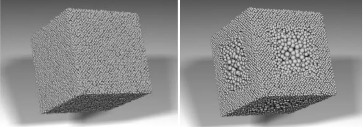
Marching cubes (MC) had seen a lot of use for many particle systems that has obscure surfaces. As a surface generation algorithm, MC algorithm gives vo-lumetric characteristics to any particle system. However, it also rounds up the sharp surface changes thus giving the material a soft and bumpy look. In this thesis, a parallel GPU implementation of MC is used. The implementation is based on Nvidia’s Marching Cubes in SDK examples [38].

In MC, there are a lot of variables that need to be calibrated for a physical model. Grid size, voxel/cell size, isovalue and sampling approach can drastical-ly change the appearance of an MC surface. To be able to adjust these va-riables, the intricate details of the MC algorithm must be known. Regarding the simulation knowing the following facts is enough.

The grid size defines the boundaries of the MC algorithm. Any particle falls off the grid is not included in surface generation. Voxel size defines the resolution of the algorithm (see Figure 3.4). Iso-value works as a measure to determine how many particles are required to consider a voxel filled and to what extent it is filled. In other words, it adjusts the triangle index that the MC algorithm accesses for triangulation. Lastly, the algorithm needs the sample data to pro-duce an iso-surface with the given iso-value.

Figure 3.4: Effects of grid size to final mesh [39]. Note: Grid size refers to voxel size in this document.

The way of sampling particle system data for MC differs a lot according to the type of simulation. For SPH simulations, a fraction of particle radius is given as a voxel size and particles fill out edges of the cubes according to

(41)

neighbor-CHAPTER 3. FLOWING AVALANCHE SIMULATION 31 ing particles density within a threshold distance. For this simulation, a simi-lar approach is taken. Depending on the amount and place of particles in a voxel, the values for the edges of a voxel are increased according to the dis-tance between the edge and the particle (see Figure 3.5 and Equation 3.18).

Figure 3.5: Contribution of a particle to sampling.

(3.18)

Where is the distance between the center of the particle and the edges of the voxel, is the total number of particles in the neighboring cells and is the mass of the particle. This equation provides a value which is inversely propor-tional to the distance from the edges of the sampling cube.

After the sampling process, marching cubes algorithm creates a surface geo-metry with the given sample data on a 128x128x128 grid resolution with voxel size of 1 unit. The CUDA MC algorithm is summarized below (see Algorithm 3.3).

(42)

1 Run voxel classification function on sample data 2 for each voxel assign one CUDA thread and do

3 Mark if voxel is empty.

4 Calculate volume value at edges 5 Calculate number of vertices in voxel.

6 End

7 End voxel classification 8 For each occupied voxel

9 Add the voxel to occupiedVoxel array 10 Add one to voxelCount

11 End

12 Run triangle generation function on occupied voxels.

13 for each occupied voxel assign one CUDA thread and do

14 Read sample data on each edge of the voxel 15 On shared memory of CUDA and do

16 Interpolate vertex coordinates and normal values.

17 End

18 Write the vertex coords. in output array. 19 End

20 End triangle generation function

Algorithm 3.3: Marching Cubes Algorithm in CUDA.

The rendering of the resulting mesh is done via GLSL (OpenGL Shading Lan-guage) shaders with the lightning scheme similar to terrain rendering as de-scribed in [45]. In these shaders, light attenuation, ambient, diffuse, specular and bump mapping is handled. In addition to this, there is a glittering post processing effect, which is based on [46], for a gleaming look (see Figure 3.6).

(43)

Figure 3.6: Flowing snow with Particle Shading and Marching Cubes, Render resolution 128x128x128.

Rendering takes just one call with the data taken from the vertex position list output of GPU marching cubes algorithm. Since the sampling of marching cubes data does not generate more than 20,000 triangles, the render call does not hinder much performance on GPU compared to the calculation of iso-value and surface generation of marching cubes algorithm. Expectedly, this is not the case for the actual algorithm runtime.

Marching cubes has a dramatic impact on performance on simulation if num-ber of occupied voxels is plenty. This, of course, is related to the numnum-ber of particles in the scene and adjoined in the flow and the method used for sam-pling. Even though it slows down the simulation, it adds the volumetric ap-pearance that a flowing avalanche requires (see Figure 3.6). Further details about performance will be given in results section.

(44)

3.3.2 Particle Shaders

In order to give the avalanche a granular look, the particles on the surface of the avalanche are rendered individually using a GLSL shader with transpa-rency enabled in addition to the marching cubes rendering. Particles are ren-dered slightly on top of marching cubes mesh, which gives a granular look to a volume of flowing snow. The size of the particles adjusts linearly according to the distance between viewpoint and particle position. With particles piling up on solid surfaces, a smoother view is generated on edges of the flowing snow (see Figures 3.6 and 3.7).

(45)

Figure 3.8: Particle rendering in avalanche simulation.

Particles are rendered as point sprites in shape of small spheres with transpa-rency color add-on flag enabled. This flag enables color accumulation on all transparent particles. For instance, when two aligned particles are observed from the camera, their illumination and color will add-up and result will show on the viewport. Consequently, this scheme creates a more vivid appearance of flowing snow on top of marching cubes rendering (see Figures 3.6 and 3.8). The rendering of particles are handled in a single call with a list of vertices as point sprites. As long as the point sprite size is not too large, particle render-ing does not put a significant burden on GPU (Less than 20 milliseconds for 524,000 particles). More detailed comparison is done in results section.

It is important to take note that rendering with transparency enabled is an effort to mimic in a holistic way the snow chunks which change shape and density during the flow. Improvements that can be made are discussed in fol-lowing chapters.

3.3.3 Terrain and Environment Rendering

Rendering done in background also has an effect on this simulation regarding marking the occurrence conditions of the avalanche. In current simulation en-vironment, the setting is on a snowy mountain, where layered snow has formed a thick layer below the avalanche zone. While the simulation takes place, terrain does not deform or change shape but provides a solid path and interacts with the particles by forming attraction bonds with them (described

(46)

CHAPTER 3. FLOWING AVALANCHE SIMULATION 36 in section 3.1.4).

For rendering the surface terrain and environment, a set of shaders are uti-lized. For lightning calculations of terrain, light attenuation, ambient, diffuse, specular and bump mapping is taken into account. Also, to give a realistic look, per pixel fog is added as a post processing effect (see Figure 3.9).

Figure 3.9: Terrain and Foggy Environment Rendering in avalanche simula-tion.

The fog is calculated on vertex shader and drawn on fragment shader by an exponential coefficient and its effectiveness on mesh color increase as the ob-jects move away from the camera. The algorithm of fog generation is shown below (see Algorithm 3.4 and 3.5).

1 for each vertex in simulation do 2 define LOG2 as 1.442695

3 define as vertex distance from camera.

4 FogIntensity 5 clamp FogIntensity between 0 and 1.

6 end

(47)

1 for each pixel in simulation do

2 Interpolate via FogIntensity, between fogColor and pixelColor 3 end

Algorithm 3.5: Fog color interpolation in fragment shader.

The render pass of the terrain is handled by the Irrlicht Rendering Engine. The method used to render the terrain is based on the LOD (Level Of Detail) rendering [52]. The algorithm creates render calls in patches and detects the unseen triangles or details via an octree structure and provides different reso-lutions of the terrain according to corresponding level of detail that increases as the distance between the viewpoint and terrain surface decreases. This al-gorithm can provide a significant improvement in terrain rendering as it di-vides terrain into specified number of patches and each patch render on its own level of detail. Thus, the variables must be adjusted according to needs or there may even be loss of performance compared to raw rendering of terrain triangles. For optimal performance, the patch size is set to 16 and the lowest level of detail is set to 5. Given this input on a 512x512 terrain, the algorithm creates 512/16 x 512/16 = 32x32 patches with 5 different sets of triangles. From 0 to 5 the Level of Detail decreases. For instance, in level 0 there are 1024 triangles in each patch. As the level increases the numbers of triangles reduce in powers of two (LVL0: 1024->LVL1:512-> LVL2:256-> LVL3:128…). Choosing a lower level of detail reduces the terrain smoothness from a distant view but greatly increases the rendering performance since the total number of rendered terrains is reduced significantly.

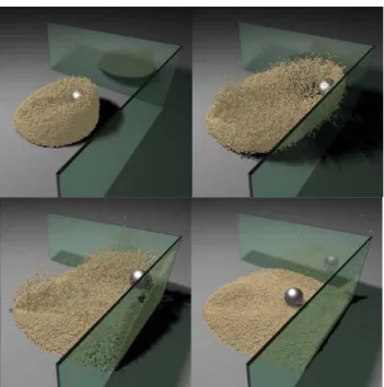
To add a bit of a realistic scenario, there is also a scenery effect in which a set of ice slates/chunks fall off the cliff and the flowing snow is released hence-forth (see Figure 4.1). These ice chunks dislodge and fall to initiate the flowing avalanche. They are predesigned in 3ds Studio MAX 2011 as a whole mesh with links that are ready to be set broken. Currently, the particles do not inte-ract with the ice slates but it is possible to handle the inteinte-raction by using me-thods such as triangle sampling or implicit sampling [53] [54].

(48)

38

Chapter 4 Results

In this thesis we have presented a method to simulate a flowing snow ava-lanche from over a mountain top to a recessive finish. To accomplish this task various methods for simulation such as particle systems and rendering me-thods such as marching cubes are utilized. To provide a faster performance, underlying hardware’s capabilities are exploited. This includes using CUDA Toolkit 3.0 (March 2010) as simulation environment and its tools for fast scanning of arrays and sorting. In addition to that, using OpenMP[54] on the CPU side further establishes a faster rendering scheme as an optimization method. OpenMP is a multi-threading API integrated into Visual Studio. It is the most simple approach of multi-threading. Its specialization is iteration loops where integration or collision detection/resolution takes place. The usage and applications are listed on [55].

First, the simulation of flowing avalanche without marching cubes and ice slates is presented (see Figure 4.1). The interaction of the particle system with terrain is described in section 3.1.4. The simulation runs on GPU, then par-ticle position data is sent to CPU to benefit from Irrlicht rendering engine util-ities in real time (see Figure 4.1). There are 128K particles in the simulation and it runs at 40 fps on a Nvidia 8800GT graphics card with CUDA Toolkit 3.0 (March 2010) installed (see Figure 4.4 and Table 4.1).

(49)

CHAPTER 4. RESULTS 39

Figure 4.1: Flowing avalanche set loose on mountainous terrain.

Another scheme (see Figure 4.2) of flowing avalanche is presented below. In this case, in addition to shaded particles, marching cubes rendering is utilized to obtain a volumetric view. Particles interact the way they do in previous scheme, only the marching cubes rendering is placed on top. There are 128K particles and it runs at 17 fps on a Nvidia 8800GT graphics card with CUDA Toolkit 3.0 (March 2010) installed (see Figure 4.4 and Table 4.1).

Figure 4.2: Flowing avalanche set loose on mountainous terrain with March-ing Cubes RenderMarch-ing.

(50)

CHAPTER 4. RESULTS 40 The last scheme (see Figure 4.3) has a set of ice slates/chunks falling before the avalanche takes place. The chunks only interact with terrain, independent from the particle system. The collision handling is done with a physics solver that works on CPU. The collision detection scheme is basically the same as particle-to-terrain interaction; however the collision resolution is slightly more complex as it takes angular acceleration into account in addition to linear ac-celeration. There are 128K particles and 232 individual ice slates that disen-tangle and slide on the terrain. It runs at 15 fps with the same system setup (see Figure 4.4 and Table 4.1).

Figure 4.3: Flowing avalanche set loose on mountainous terrain with March-ing Cubes RenderMarch-ing and ice chunks.

It is not very difficult to sample the ice meshes and create a particle-to-particle coupling. The possible improvements to this scheme are discussed in conclusion part of the thesis.

Some of the technical variables possess great significance regarding simula-tion performance. For instance, available graphics card memory defines the grid resolution of the Marching Cubes algorithm and number of particles that can reside on GPU memory for simulation. In addition to this, number of CU-DA cores and number of threads per block in a GPU directly involves the number of threads that can be run in the simulation, which in turn will be

(51)

CHAPTER 4. RESULTS 41 much faster as threads can share the load. Also, maximum register size pro-vides low latency access to small data which enables faster access of tempo-rary variables. The abovementioned features of system computer can be seen in Figure 4.5.

This implementation of flowing avalanche simulation can provide interactive frame rates for 512K particles. This is mainly thanks to the parallel architec-ture of a GPU and avoidance of serialization of processing. Surely, the choice of the particle integrator and its variables, usage of rendering schemes are al-so a decisive factor. Alal-so, there are certain factors such as marching cubes particle data sampling that can change performance a lot if performed wisely. For instance, by performing sampling on CPU and dumping the data back to GPU while it is sorting the particles might avoid CUDA core stalls and im-prove performance.

Figure 4.4: Simulation performance in frames per second with different sizes of particle sets and types of rendering.

0 10 20 30 40 50 128K

256K 512K 1024K

Frames per Second

N u m b e r o f Par ticl e s

Simulation Performance on Nvidia 8800GT

MCubes+IceChunks+Particle

MCubes + Particle

(52)

CHAPTER 4. RESULTS 42 Number of Particles Particle Only Render Particle and Marching Cubes Render Particle, March-ing Cubes, Ice chunks Render Memory Consumption 128K 40 FPS 17 FPS 15 FPS 110MB-250MB-255MB 256K 23 FPS 12 FPS 10 FPS 120MB-260MB-265MB 512K 12 FPS 6 FPS 5 FPS 150MB-290MB-295MB 1024K 6 FPS 4 FPS 3 FPS 190MB-330MB-335MB

Table 4.1: Exact values of simulation performance in frames per second with different sizes of particle sets and types of rendering with memory consump-tion.

System Specifications

CPU Model Intel Q6600 @ 3.0ghz

Memory Size/Type/Clock 3 GB / DDR2 / 1333Mhz

GPU Model Nvidia 8800GT G92

Memory Size/Type/Clock 512 MB / DDR3/ 950Mhz

CUDA Cores 112

Max Threads Per Block 512

Max Registers Per Block 32768

Memory Bandwidth 60.8 GB/sec

Simulation of a flowing snow avalanche using molecular dynamics

SIMULATION OF A FLOWING SNOW

AVALANCHE

USING MOLECULAR DYNAMICS

ABSTRACT

SIMULATION OF A FLOWING SNOW AVALANCHE

USING MOLECULAR DYNAMICS

ÖZET

ÇIĞIN MOLEKÜLER DĠNAMĠK YÖNTEMĠ ĠLE

BENZETĠLMESĠ

ACKNOWLEDGMENTS

Contents

List of Figures

List of Tables

Chapter 1

Introduction

1.1 Definition of an Avalanche

1.2 Simulation Requirements of a Flowing

Snow Avalanche

1.3 Snow Avalanche Models in Literature

1.4 List of Symbols

1.5 Thesis Outline

Chapter 2

Overview of Related Methods

2.1 Molecular Dynamics Method

2.2 Smoothed Particle Hydrodynamics

2.3 Parallelization of Physical Simulation of

Particles

Chapter 3

Flowing Avalanche Simulation

3.1 Particle System Basics

3.1.1

Inter-particle Collision Detection

3.1.2

Inter-particle Collision Resolution

3.1.3

Integration Step

3.1.4

Terrain Collision Detection and Resolution

3.2 CUDA and Simulation Optimization

3.2.1

CUDA (Compute Unified Device Architecture)

3.2.2

Utilization of CUDA in Simulation

3.3 Rendering

3.3.1

Marching Cubes

3.3.2

Particle Shaders

3.3.3

Terrain and Environment Rendering

Chapter 4

Results

Simulation Performance on Nvidia 8800GT

System Specifications