^ 9 9 3
SCHcDuUíil
• « «i* é J J 'M*' ^ ti^'V t» 'ІК/
Γ2Ι>· TC' ΤΉ 3 2>SFÁJLTi¿E¿-iT Oi? ІЖ /иЗТ
; '^'"-■'3,, ІікТЗТіТШЗ ¿i? S i IG IIÎS S ItlH ü ¿_'
T? 2:31XEÍ."T
İBTZAİ ?TL31ILi¿iBKT OiF ΊΈ2. RBQ’UïIi
ТВШ. BEGUBE Э? OF ОСІШІСВ
SCHEDULING W ITH A RTIFICIA L NEURAL
N ETW O R K S
A THESIS
S U B M m ’El) 'I'O THE DEPAHTMEN1' OE INDHS^'mAE ENCHNEERINC AND 'J'HE INSTITUTE OF ENCHNEERINO AND SCIENCES
OE BILKEN'r UNIVERSITY
IN I’ARTI A L EULFILLMENT OE THE REQUIREMENI'S FOR THE DI'XIREl·: OF
MASI'ER OE SCIENCI·
ih iv u , 1
By
Burçkaan Gürgüiı
June, 1993
I certify that I have read this thesis and that in my opinion it is fully adequate, in sco])e and in quality, as a thesis for the degree of Mastei- of Science.
'“A.
i-T
Asst. Prof. Ihsan Sabuncuoğlu(Principal Advisor)
I certify that I have read this thesis and that in my opinion it is fully adequate, in scope and in quality, as a thesis for the degree of Master of Science.
Assoc. Prof.'^evdet Aykanat
I certify that I have read this thesis and that in my opinion it is fully adequate, in scope and in quality, as a thesis for the degree of Master of Science.
Asst. Prof. Selim Aktiirk
Approved for the Institute of Engineering and Sciences; Prof. Mehmet B|^i<iy
ABSTRACT
SCHEDULING WITH ARTIFICIAL NEURAL
NETWORKS
Bui'(;.kaan Ciiirgun
M.S. in Industrial Engineering, Supervisor: Ihsan Sabuncuogiu
June 1993
Artificial Neural Networks (ANNs) attem pt to emulate the massively par allel and distributed processing of the human brain. They are being examined for a variety of problems that have been very difficult to solve. The objec tive of this thesis is to review the current applications of ANNs to scheduling problems and to develop a parallelized network model for solving the single machine mean tardiness scheduling problem and the problem of finding the minimum makespan in a job-shop. The proposed model is also compared with the existing heuristic procedures under a variety of experimental conditions. Keywords: Neural Networks, Scheduling, Tardiness, Makespan.
ÖZET
YAPAY SİNİR AĞLARI İLE ÇİZELGELEME
Burçkaaıı Gürgün
Endüstri Mühendisliği Yüksek Lisans Tez Yöneticisi: Ihsan Sabuncuoğlu
Haziran 1993
Yapay Sinir Ağlan (YSA) insan beyninin muazzam paralel ve yayılım.^ işleyişini uyarlamaya yöneliktir. Bunlar çeşitli çok zor ])roblemler için İnce lenmektedir. Bu tezin amacı YSA’nin çizelgeleme problemlerine mevcut uygu lanışlarım incelemek buna ek olarak tek makineli çizelgeleme problemlerinde ortalama gecikmeyi en aza indirmeyi hedef alan ve çok makineli çizelgeleme problemlerinde en son kalan işin tamamlanış zamanını en aza indirmeyi hedef alan paralelleştirilmiş bir ağ örgüsü modeli geliştirmektir. Önerilen metod mev cut algoritmalarla karşılaştırılmıştır.
Anahtar Kelimeler: Sinir Ağlan, Çizelgeleme, Gecikme, Son İşi Tamamlama.
A C K N O W LED G EM EN T
1 would like to thank to Asst. Prof. Ihsan Sabuncuoglu for his supervision, guidance, suggestions, and patience throughout the development of this thesis. I am grateful to Assoc. Prof. Cevdet Aykanat and Asst. Prof. Selim Aktiirk for their valuable comments.
Also, I would like to thank to my family and all my friends. Special thanks to Didem Okutgen, Taner Şekercioğlu and Müjdat Pakkan, who apjreared to be around when I was in need.
C ontents
1 INTRODUCTION 1
2 ARTIFICIAL NEURAL NETWORKS 3
3 LITERATURE REVIEW 12
3.1 Hopfield Model for Scheduling Problems 12 3.2 Other ANN Approaches 16
4 THE PROPOSED APPROACH 18
4.1 Single Machine Mean Tardiness Scheduling Problem ... 22 4.1.1 Application of the Proposed Method 23 4.1.2 Experimental Results & Com parisons... 28 4.2 N \M .Job-shop Scheduling Problem Minimizing Makespan 35 4.2.1 Application of the Proposed Method 36 4.2.2 Experiments L· R e su lts... 46
5 CONCLUSIONS 48
A 50
List o f Figures
2.1 Schematic drawing of a typical neuron... 4
2.2 A typical multilayered neural network... 5
2.3 Schematic processing unit from an artificial neural network. 6 2^4 Sigmoid function... (i
2.5 A back propagation ANN... 9
2.6 The Hopfield Type ANN, used for TSP... 10
4.1 A neural matrix and the resulting schedule... 19
4.2 Typical Hopfield network and the proposed network...21
4.3 The schedule generated by the proposed approach for the sample problem... 28
4.4 The geometric shapes of data types... 30
4.5 The string population of size 3 for GA and forming a child. . . . 34
4.6 The proposed network for 4|2 job-shop scheduling problem. . . . 37
4.7 The machine routes of the operations of job i and job j . 38 4.8 A neuron matrix in which the first and second positions are include in the PSP set... 39 4.9 The current schedule generated by the network to calculate El. 44 4.10 The schedule generated by the network for the 3|2 job-shop prob
lem. 45
List o f Tables
4.1 Results of WI and the proposed network for single machine mean tardiness scheduling p r o b le m :... 29 4.2 Confidence interval tests for the difference between WI and the
proposed netw ork:... 31 4.3 Confidence interval tests on the relative performance of the pro
posed network and WI for sizes 50 and 100 jo b s :... 31 4.4 Confidence interval tests on the varying tf values for the pro
posed network and WI for sizes 50 and 100 j o b s :... 32 4.5 Confidence interval tests on the varying rdd values for the pro
posed network and WI for sizes 50 and 100 jo b s :... 32 4.6 Comparisons of the results of the proposed network and CA
applied to it, for the problem size of 50... 33 4.7 Comparison of job-shop scheduling problems using makespan
criterion... 47 A.l Results of 1|50 job-shop problem for rectangular shaped data: 51 A.2 Results of 1|100 job-shop problem for rectangular shaped data: . 52 A.3 Results of 1|50 job-shop problem for linear-f shaped data: 53 A.4 Results of 11100 job-shop problem for linear-|-shaped data: . . . 54 A.5 Results of 1|50 job-shop problem for linear- shaped data: . . . . 55 A.6 Results of 1|50 job-shop problem for v-shaped- data: 56 A.7 Results of 1|50 job-shop problem for v-shaped-|- d a t a : ... 57 A.8 Results of IjlOO job-shop problem for v-shaped-)- data: 58
C hapter 1
IN T R O D U C T IO N
Scheduling occurs in a very wide range of economic activities. It always in volves accomplishing a number of things which tie up various resources for periods of time. The resources are in limited supply. The things to be ac complished may be called jobs and are composed of elementary parts called
operations. Each activity requires certain amounts of specified resources for
a specified time called the processing time. Resources also have elementary parts, called machines., cells, tran.spori, delays, etc. Scheduling problems are often complicated by large numbers of constraints. For exam])le, there may be precedence constraints connecting activities that specify the processing se quences of activities within a job.
A scheduling system dynamically makes decisions about matching activi ties and resources in order to finish jobs needing these activities and resources while satisfying the defined constraints. The purpose of a scheduling system is to maximize or minimize a specified objective. There are numerous and often conflicting objectives in the context of scheduling. These can be classified into (1) criteria based upon completion times, (2) criteria based upon due dates and (3) criteria based upon inventory costs and utilizations.
Job-shop scheduling is considered as the general case of scheduling prob lem where n jobs, and m machines are modeled (rtl??;. job-shop). Except in relatively simple cases, determination of an optimum schedule is extremely dif ficult due to the combinatorial nature of job-shop scheduling problems. The single machine mean (total) tardiness scheduling problem is a special case of this problem. It has also been proved to be NP hard in the ordinary sense.
CHAPTER 1. INTRODllCriON
As a consequence, near optimal solutions are considered to be good enough for real life problems. In the literature, a number of heuristic approaches have been proposed to solve these problems, ranging from priority dispatching rules to integer programming formulations.
The recent developments of neural networks have also motivated some re searchers for applications of Artificial Neural Networks (ANN) to scheduling problems. Several Hopfield type networks and its variants have been pro])osed to solve job-shop scheduling problems as well as other combinatorial optimiza tion problems.
Objective of this thesis is to review the current applications of ANN to scheduling problems and to develoj) a parallelized network model for solving the single machine mean tardiness scheduling problem and the problem of find ing the minimum makespan in a job-shop.
In chapter 2, a brief history of ANN and its applications are given. This is followed by a literature review of ANN pertaining to scheduling. In chap ter 4, a neural network is developed for the single machine total tardiness scheduling problem and the job-shop problem with the makespan criterion. Performance of the proposed network is compared with the two phase algo rithm of Wilkerson-Irwin [1] for the single machine case. The results for the job-shop is compared with the known values (or upper bounds) of various job-shop problems. Chapter 5 contains concluding remarks & suggestions for further research.
C hapter 2
AR TIFIC IA L N E U R A L
N E T W O R K S
Artificial neural systems (ANSs) are mathematical models of theorized mind and b rain activity. AN.Ss ai-e refe rre d to as n e u ra l n e tw o rk s, connectionism, adaptive systems, adaptive networks, ANNs, neurocomputers, and parallel dis tribution processors. ANN provides a coni])uting architecture whose applica tions and power increases steadily. The new computing architecture, inspired by the structure and functions of the brain is radically different from the com puters that are widely used today. Conventional computers rely on algorithm- based programs that operate serially, are controlled by com])lex central pro cessing unit, and store information at addressed locations in the memory. The brain relies on highly distributed representations and transformations that op erate in parallel, have distributed control through billions of highly intercon nected neurons or processing elements and appear to store their information in variable strength connections called synapses. Some of the fundamental com ponents and functions of the brain are as follows;
-Neurons: the small units of the brain that are capable of simple processing (Figure 2.1).
-Dendrites: the neuron branches that form a network connecting neurons. -Synaptic connections; the connections through which electric charge passes from dendrites to neurons.
-Axon: the long neuron branch that carries the output (chemical or electrical) of a neuron to the network of dendrites.
-Excitation and inhibition of neurons: chemical or electrical inputs originating from sensing external stimulations or other neurons either excite or inhibit a
СНА PTER 2. А RTIFICÏA L NE U RA L NETWORKS
Figure 2.1: Schematic drawing of a typical neuron. neuron; that is, they have either positive or negative effect on it.
-Neuron activity: Once the excitation level of a neuron rises beyond a thresh old, the neuron fires and sends out a chemical or electrical output; the strength of the neuron’s activity is the frequency per second of the neurons firing. -Massive parallelism: A neuron has up to 10,000 synaptic connections. The human brain is estimated to have 10" neurons. The processing of the human brain is massively parallel.
ANN is a directed graph with weighted edges that is able to store patterns by changing the edge weights and is able to recall patterns from incomplete inputs. Key elements of ANN are; the distributed representation, the local operations, and nonlinear processing. These attributes emphasize two of the primary applications of ANNs; situations where only a few decisions are re quired from a massive amount of data and situations where a complex nonlin ear mapping must be learned. A typical ANN consists of:
-Layers: the most common structure of ANN contains an input layer, an out put layer and possibly additional (hidden) layers. The input layer contains nodes that receive input data of activated and inactivated (boolean) states. The input received from the environment may be encoded to the input layer. The input data is transferred to the hidden layei' by weighted interconnections non-linearly. There might be more than one hidden layer due to design. The processed data is transferred to the following hidden layers and finally to the output layer. The output layer, like the input layer contains activated and inactivated states of neurons. The output layer can be decoded as a solution
CHAPTER 2. ARTIFICIAL NEURAL NETWORKS ^ „®2,SENSOR "C A T” (ID-s e n (ID-s o r "D O G " ..!5 , SENSOR "R AB B IT"
Figure 2.2: A typical multilayered neural networl of the problem (Figure 2.2).
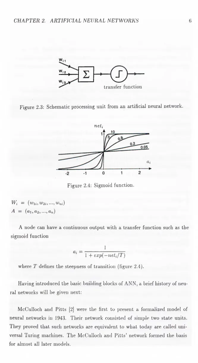
-Nodes: each layer contains a number of nodes. A node corresponds to a neuron. Similar to the neurons, each node i has an activation (firing) value a,·, that is between 0 and 1.
-Connections: some nodes in the network are connected by some connections. A connection corresponds to synaptic connections and dendrites (Figure 2.3). -Weights: each connection from node j to node i has a weight of the value of these activities is between 0 and 1.
-Node’s net input: the net input to a node i is:
neti = J 2aU nodes connected to i + exUliputi
where extinputi is the environmental input to node i. The mathematical ex planation of this sum is that it is the inner product of two vectors IT, and A.
CHAPTER 2. ARTIFICIAL NEURAL NETWORKS
w,2
w13.
<£>
transfer function
Figure 2.3; Schematic processing unit from an artificial neural network.
neti
Figure 2.4: Sigmoid function.
Wi = {lVu,W2i,...,Wni) A = (fi] , fl2) •••5
A node can have a continuous output with a transfer function such as the sigmoid function
_________ 1________
' 1 + exp{—neti/T )
where T defines the steepness of transition (figure 2.4).
Having introduced the basic building blocks of ANN, a brief history of neu ral networks will be given next:
McCulloch and Pitts [2] were the first to present a formalized model of neural networks in 1943. Their network consisted of simple two state units. They proved that such networks are equivalent to what today are called uni versal Turing machines. The McCulloch and P itts’ network formed the basis for almost all later models.
CHAPTER 2. ARTIFICIAL NEURAL NETWORKS
In 1949, Hebb [3] suggested that an assembly of neurons could learn by strengthening the connections between two neurons whenever they were both simultaneously excited. This learning scheme was known as the Hebb prescrip tion.
Rosenblatt developed in the .^O’s a simple formalized model of a biolog ical neuron ba.sed on the McCulloch-Pitts’ neurons and Hebb’s prescription. His model, which he called Perceptrons was described in his book Principles of Neurodynamics [4] from 1962. Rosenblatt’s Perceptrons consisted of sen sory units connected to a single layer of McCulloch-Pitts’ neurons. Rosenblatt proved a theorem which stated that training of perceptrons to classify jjatterns into linearly separable classes, converged in a limited number of steps.
In 1960, Widrow and Hoff [5] published a paper in which they proposed a McCulloch-Pitts’ type neuron called adaline (Adaptive linear neuron). The only (and important) difference was the pro])osal of a learning algorithm.
In 1969, Minsky and Papert [6] analyzed the single-layer perceptrons in their book Perceptrons. They proved that such networks are not capable of solving the large class of non-linear separable problems. They recognized that the extension of hidden units (neurons that were neither input nor output) would overcome these limitations, but stated that the problem of training such intermediate units was probably unsolvable. The impact of their work was very strong. The interest in ANN practically disappeared; only a few researchers such as Malsburg, Grossberg, Kohonen and Anderson remained in the field.
The field attracted substantial attention again in the beginning of 80’s. In 1982, Hopfield [7] demonstrated the formal analogy between a net of neuron-like elements with symmetric connections and a spin glass. Hopfield showed that the network could be trained as an associative memory using Hebb’s rule for synaptic weight modification. These networks are now known as Hopfield nets. Hopfield Neural Networks are highly interconnected networks that minimize a given energy function by local perturl)ations until the network becomes stable at a local or global minimum. The interconnection weights are determined by the energy function which represents the objective function. The Hopfield
network is sini])ly a single layered fully connected network that evolves to a stable state through time. The evolution is carried out by randomly firing the neurons of the network using the sigmoid function. The stable state reached at the end, is close to the minimum of the energy function (E) of the network,
CHAPTER 2. ARTIFICIAL NEURAL NETWORKS 8
s = - 5 E Wijaidj
Hence, in order to load the desired energy function to the network the inter connection weights Wij must be adjusted due to the objectives and constraints.
In the same year Kohonen [8] ])ublished an article describing an artificial neural network based on self organization. The idea was to make use of the fact that sensory signals were represented as two dimensional images or maps in the cortical system. Kohonen formulated a model with a self organization mechanism which used a neighborhood function to define the area in which to cluster similar input signals. This way of clustering was initially studied by Malsburg [9] in 1973.
In 1983, Hinton and Sejnowsky [10] extended Hopfield’s model with hidden units and stochastic dynamics. They called their network a Boltzmann ma chine.
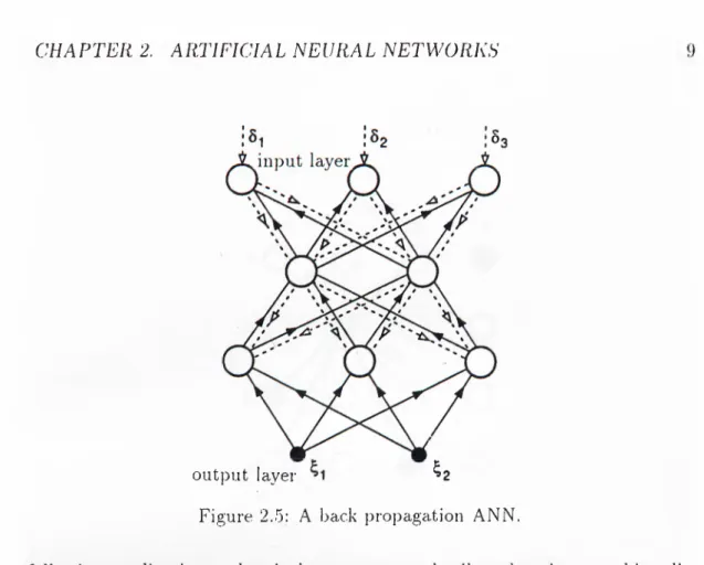
About two years later Rumelhart, Hinton and Williams [11] derived a learn ing algorithm for perceptrons networks with hidden units based on Widrow and Hoff learning. Their learning algorithm was called back propagation and is now the most widely used learning algorithm (Figure 2.5).
Much effort had been put into the analysis and further development of the back propagation (BP) algorithm since then. This algorithm has been applied to a great variety of problems, including recognition of protein structures, hy phenation of English words, speech recognition, image compression, com])uting shape from shading and j^redicting chaotic time series [12].
There are also other neural network architectures which have been devel oped over the time. These include; counter ];>ropagation, hamming, Kohonen feature ma]), bi-directional associative memory, BP shared weights, BP recur rent, multi layer adaline and Potts [13]. The.se networks have been used in the
CHA PTER. 2. AR.T1FICIA L NELIRAL NETWORKS
;o3
output layer ^2
Figure 2.5: A back propagation ANN.
following applications: chemical process control, oil ex])loration, machine di agnostics, medical diagnostics, anti-body detection, classifying tissue samples, marketing, financial modeling, forecasting, risk management, credit apjjlica- tion rating, bankruptcy prediction, bank card found, hand written character recognition, speech recognition, adaptive flight control, sonar signal processing, monitoring rocket valve o].)erations, coin grading, race-track betting, dealing with noisy data, pattern mapping, pattern completion, etc.
One of the new and promising application of ANN is to find near optimal solutions for the combinatorial optimization problems. With a few exceptions in all ANN applications to the optimization problems, Hopfield Neural Network (HNN) is used. .Since the travelling salesman problem (TSP) is one of the fa mous N P hard problem in a classical optimization literature, most of the ANN applications are directed to the TSP problem [14,15,16,17,18,19,20,21,22,23]. For that reason, a brief summary of TSP applications will be given before in vestigating ANN in the context of scheduling problems.
In most ANN applications to the TSP, the problem is mapped into a 2D matrix using N'^ neurons, where N is the number of cities. Neurons are rep resented in the matrix as .t, f = 1 ,...,A ^ The first index represents the
city name and the second represents the position of the city in the tour. A permutation matrix is required to obtain a feasible solution. The cost function
CHAPTER 2. ARITFICIAL NEURAL NETWORKS 10
Stop
1 2 3 4
Figure 2.6: The Hopfield Type ANN, used for TSP.
and the constraints of the problem are coded into the network via the inter connection weights Wxi^yj corresponding to and (lyj [24] (figure 2.6). E = A /2
AH12 ^,· ^3, (ixidyi +C/2{J2x T,iO,xi - n f
AD j2 ^2ix '^y:^x X2i ^xy^xi{^y,i-\-l "F —l)
The interconnection matrix defined by the above energy function is as fol lows :
^xi,yj A6xy(^l B6ij(^\ ^xy} C· Ddxy(^6ji^\ “b (Sij = 1 if i = j and 0 otherwise)
A, B, C, D are problem dependent scaling constants. The terms of A, B, C
are hard constraints in order to have a feasible solution, and the term of D is the soft constraint for satisfying the objective function.
In general, there are two basic problems rising up with current Hopfield Neural Networks applications: (1) the energy function gets stable at a local minimum and cannot even find feasible solutions because of the comj^lexity of
CHA PTER 2. A RTIFICIA L NEURA L NETWORKS 11
the energy function, (2) computational reciuirements of the network dramati cally increases as the problem size gets larger when the network is emulated on the existing computers. In such cases, an annealing a])])roach usually is used to escape from the local minima at a cost of increased computational time. Several annealing methods have been recommended in the literature. Some of them are: Simulated Annealing (SA), Fast Simulated Annealing (FSA), Mean Field Annealing (MFA), Rejection-less Simulated Annealing (RSA), etc. In general, ANN applications to TSP finds optimal and near optimal results for sizes of less than 10 cities [14,15,16,17,18]. However, network does not converge to a feasible solution when the size increase. In fact, if the ratio of the weights of hard (feasibility) constraints to soft (objective function) constraints is in creased feasible solutions might be obtained at a cost of deteriorating cpiality of the solutions.
Hopfield Neural Networks have also been used for various other combina torial optimization problems such as graph partitioning, graph coloring, graph flow, scheduling, resource allocation, load balancing fc programming j)aral- lel computers, data deconvolution, control, stress measurement, integer pro graming, solving equations Sz optimizing functions, pattern matching, image processing and signal processing [13]. In most of the ANN applications to combinatorial optimization problems similar difficulties (a very complex ANN with infeasible solutions) arise when the size of the problem increase. Hence, researchers either deal with the special cases of these j)roblems, or they modify the ANN in order to obtain good feasible solutions.
C hapter 3
L IT E R A T U R E R E V IE W
There are various ANN architectures proposed in the growing literature of ANN scheduling. These networks can be classified into (1) neural networks based on the extension of Hopfield model and (2) other ANN approaches such as a backpropagation network. Thus, the literature review will be made according to this classification.
3.1
H o p fie ld M o d e l for S c h e d u lin g P r o b le m s
Researchers has first attempted to solve the scheduling ])roblems using the ex tension of the Hopfield network. In this context, Picard and Queyranne [25] proposed that the time-dependent traveling salesman ])roblem may be stated as a single machine scheduling problem in which n jobs have to be processed at minimum cost on a single machine. The set-up cost associated with each job depends not only on the job that precedes it, but also on its position (time) in the sequence.
Gulati Sz Iyengar [26] proposed a Hopfield model using a mapping of the uniprocessor scheduling problem with hard deadlines, and task priorities. The problem is mapped into a Hopfield Neural Network with nlog{np) neurons. Where n is the number of jobs and Up indicates the total processing times of all jobs. In order to reduce complexity the time axis is scaled logarithmically. The neuron matrix shows the starting times corresponding to each job. The energy function to be encoded to the network has four terms ; term for tardi ness (Et), term for waiting time (Ew), term for overlapping (Eq) and term for
CHAPTER :J. LITERATURE REVIEW 13 will be : Etotai = E'r + Ew + Eo + Ep. In the simulations, Fast Simulated Annealing· (FSA) is used to obtain near optimal solutions for a 20-job problem.
Arizono and Yamamoto [27] proposed a solution method using an ANN for the uniprocessor scheduling problem to minimize the total flow time under the just-in-time production environment. Their ANN architecture was also an extension of the Hopfield model, so called Gaussian machine model. Their network generated near optimal solutions for problems of 10 jobs.
Fang and Li [28] proposed methods for the design of competition based neural networks for combinatorial optimization problems. They designed and presented the energy functions of the network for the single machine tardiness problem with unit processing times and different deadlines. They reported op timal solutions for 7, 10, 15 and 20 job problems.
The first three methods discussed above assumed a single processor (or sin gle machine). There are also studies which investigates applications of ANN to job-shop scheduling problems. These are as follows:
Lo and Bavarian [29] extended the two dimensional Hopfield network used for TSP problem to a three dimensional neural matrix where the z-axis rep resents the jobs, the x axis represents the machines and the y-axis represents time. In their approach, they used this extended network for solving job-shop scheduling problems with deadlines and limited processing times. They solved several problems. In their computation experiments, they obtained near opti mal results for problems of 10|3 and 6|3. However, this approach has limited applications, because the size of network and the number of connections in crease enormously when the number of machines or jobs increase.
Foo and Takefuji [30] also proposed a Hopfield net by mapping the n\7u job-shop scheduling problem with the objective of minimizing mean flow time on a 7Tin by (77171-f 1) 2D neuron matrix similar to those for .solving the TSP. In their formulation, constant positive and negative biases are applied to specific neurons as excitations and inhibitions to enforce the operation precedence re lationships. At the convergence of neural network, the solution to the job-sho]) problem is represented by a set of cost function trees encoded in the matrix
CHAPTER 3. LITERATURE REVIEW H of stable states. Each node in the set of trees rejjresent a. job, and each link represent the interdependency between jobs. The cost attached to each link is a function of the processing time of a jiarticular job. The starting time of each job is determined by traversing the jjaths leading to the root node of the tree. A computation circuit compute the total completion times (costs) of all jobs, and the cost difference is added to the energy function of the stochastic neural network. Using a simulated annealing algorithm, the temperature of the system is slowly decreased according to the annealing schedule until tlie energy of the .system is at a local or global minimum.
There are three basic (hard) constraints to be encoded in their neural net work model to have a feasible solution. These conditions are: (1) no more than m number of jobs are allowed to start at time 0, (2) self-dependency on each operation is not allowed (an operation can occur only once in the schedule) and (3) precedence relationships between operations must be obeyed. If there are n jobs and m machines available then at most m jobs could start indepen dently at time 0. Constraint of type (1) is used when n > m. In this situation, randomly chosen m out of n unique jobs start at time 0. Constraint of type (2) is necessary to avoid self-recurring dependency paths. This condition ’ enforced by placing strong inhibitions (negative bias) at appropriate neurons so that these neurons would not trigger. (Constraint (3) is used to preserve the precedence relationships. Based on the problem formulation the global energy function which contained the constraints of a job-shop problem was defined as: E = +A /2 ^xiO-xj + B/2{Y^x ^Xi —
A and B are problem dependent scaling constants of the energy function. The first term is zero if and only if each row in the matrix of neurons does not contain more than one firing neuron. The second term was zero if and only if there are z neurons being turned on in the whole matrix of neurons. The interconnection (conductance) matrix defined by the above energy function is as follows: wxi^Yj = —A6x Y{ l —Sij) — B. The energy function, composed of the hard constraints and the cost of total completion times of all jobs was applied to an annealing schedule. The method had given feasible and near o])timal solutions for 4|3 job-shop problems.
an integer linear programming form with the cost function of the total comple tion times of all jobs. They coded the integer linear jrrogram to the Hojrfield network and solved the same size problem above.
This integer linear programming neural network (ILPNN) for the job-sho]) problem handles the following mixed-integer linear programming problem: Minimize
E n c
1 = 1 *- lA.-! Subject to
•Sa,· - 'S/i > if operation (i,j-l,h) precedes (i,j,k)
Spfc - .S^. -f / / * (1 - ¡(/¿pA;) > U j k i > l , P<n, 1 < A: < m
Sik - Spk + H * xyipk > ip<,k i> l, P<n, 1 < k < m
Sik > 0
Vipk = 0 07· 1
where
ki = The machine which the last operation of job i was assigned. Sik = The starting time of operation k of job i.
t-jf. = The duration of operation j of job i at machine k.
In this formulation, there is a total of xnrV constraints for the network. The constraints are encoded to the ILPNN using nm.{nm-\-1 )/2 neurons. Their computational studies based on solving the linear differential ecpiation of neural network showed that the ILPNN approach produced optimal or near optimal solutions, although it does not guarantee the finding of optimal solutions.
Zhou, Cherkassky, Baldwin, and Olson ([32] and [33]) further improved the performance of ILPNN for job-shop scheduling problems. In their ajjproach, the indices indicating operations and machines are unified to have a integer programming relaxation of the problem. They simulated their network on 2[3, 4[3, 5|3, 6|6, 7(7, 10(10 and 20|20 job-shop problems and found nejar optimal solutions.
CHAPTER. 3. LITERATURE REVIEW 15
Hulle [34] and [35] also solved the job-shop problem by using a goal pro gramming network. This network finds the ojrtimal goal programming solution. The solution is obtained by repeatedly performing goal programming relax ations and binary adjustments until convergence. According to this method.
CHAPTER 3. LITERATURE REVIEW IG an optimal solution for the problem cannot be guaranteed, but the solution is always feasible with respect to the constraints of the job-shop problem.
Finally, Gislen, Peterson and Sodeberg [36] extended the approach of Potts neural networks using mean field annealing algorithm to real life scheduling problems. They solved the problem of scheduling of the teachers to courses in a high school. The results of their exj^eriments were very successful with respect to quality of the solution and CPU time.
3 .2
O th e r A N N A p p r o a c h e s
The ANN applications discussed so far are all based on the extension of Hop- field neural network. In the recent literature, there are also ANN applications which use other netwoik architectures.
For example, Chryssolouris, Lee, and Domioese [37] modeled a manufac turing system hierarchically. They develo])ed a back propopagation network to establish adequate weights on the criteria used in the work center level of the manufacturing system based on performance measure goals for the job shop.
Carlos and Alptekin [38] proposed an integrated (ex])ert systems and ANN) scheduling system in which a back])ropagation network was used to rank some scheduling rules based on the current status of the system and job characteris tics. The outputs (relative weights) of the network are further analyzed by an expert system to generate schedules.
In both of the above studies, ANNs were mainly used for finding appropri ate weights of either scheduling rules or decision making criteria, rather than generating schedules directly by a backpropagation network.
Osman and Potts [39] used the simulated annealing a])]uoach for the per mutation flow-shop problem. The results indicated that SA improved the per formance measures better than known constructive analytical algorithms.
Finally, Laarhoven, Aarts and Lenstra [40] proposed an approximation al gorithm for the problem of finding the minimum makespan in a jol)-shop. The
CHAPTER :i LITERATURE REVIEW 17
algorithm is based on simulated annealing. The annealing procedure involves the acceptance of cost-increasing transitions with a. nonzero probability to avoid getting stuck in local minima. In their work, it is proved that the algorithm asymptotically converges in ])robability to a global minimum solution, despite the fact that the Markov chains generated by the algorithm are generally non irreducible. Computational experiments show that the algorithm can find rel atively shorter makespans for 6|6, 20|5, 10|10, 10|15, 10|20, 10|30, 5|10, 5|1.3, 5|20 and 15|15 job-shop problems.
From this brief literature review, the following observations can be made: (1) The majority of ANN applications to scheduling problems are based on the Hopfield neural network. Although these applications yield promising re sults, the existing approaches still inherit the problems of ANNs in the TSP applications. (2) When the size of the problems increases, the network size and computational requirements increase enormously and ANN does not re sult with a feasible solution. (3) The approaches are not compared with other existing scheduling algorithms. (4) The iipproaches are diiected to simple in stances of scheduling ])roblems.
In order to develop a general and better network model, the ANN may need to be simplified by attaining feasibility of the network with an external inter ference so that the hard constraints are dropped from the energy function and feasibility is guaranteed by the external processor. Further simplifications and improvements of the network might be achieved by calculating the energy func tion (which includes only the cost terms) without using the interconnections but rather using a cost calculating processor. Although, these modifications can radically divert from the classical ANN approaches, they might be useful in overcoming the problems of ANN in scheduling and other combinatorial opti mization problems. In the following chapter, these modifications will lie made to develop the proposed parallelized neural network model. The resulted net work will be applied to the single machine mean tardiness scheduling problem, and general job-shop scheduling problem with the makespan criterion.
C hapter 4
TH E PR O P O SE D
A P P R O A C H
The basic motivation behind this research is to eliminate some of the limitations of the Hopfield neural network and propose a new neural network architecture for scheduling problems. The Hopfield model, when applied to combinatorial optimization problems are not capable of solving relatively large size i)roblems. The reason for that is the size of the ANN which grows enormously as the prob lem size increases. In order to alleviate this i)roblem, the Hopfield network will be modified. Specifically, the energy function will be simplified by taking out feasibility constraints. The proposed method consists of a parallelized Hopfield model. The network is monitored and controlled by an external processor. As a result most of the interconnections of the Hopfield model are eliminated. In the proposed method, the energy function is just the scheduling cost function and its value is computed by the external processor. In most of the Hopfield applications, local energies corresponding to the neurons are calculated, but in the proposed method total energy of the network is computed.
While constructing the architecture of the proposed model, a sequence of jobs is represented by a nxn neuron matrix (Figure 4.1). The neuron matrix
is interpreted as follows : each row indicates a job and each column indicate a position in the sequence (or schedule) of the jobs. As each job can be placed in only one position, the final feasible solution matrix must have only one ac tivated neuron at each row and column and the rest of the neurons must be inactivated (i.e., a permutation matrix). As a notation, the state of a neuron
aij = 1 when it is activated (i.e., job i is assigned to the jth position in the
CHAPTER 4. THE PROPOSED APPROACH 19
U\2 ¿¿13 ■ 1.00 0 .0 0 0 .0 0 ■
<'¿21 a-22 ¿¿23 = 0 .0 0 1.00 0 .0 0
¿¿31 (1-32 ¿¿33 . 0 .0 0 0 .0 0 1.00
J1 J2 J3
Figure 4.1: A neural matrix and the resulting schedule.
schedule), «¿j = 0 when it is inactivated (i.e., job i is not assigned to the jth position in the schedule). If 0 < «¿j < 1, then job i is assigned to the jth position with a probability Uj-j. Thus, in the single machine case, obtaining the final network in the form of a permutation matrix produces a feasilde solution for the problem.
In general, most of the existing neural networks, es])ecially the Hopfield models use inhibitory connections in order to achieve the feasibility. In the proposed approach, this is partially achieved by normalization (i.e., dividing activation values of each neuron by the sum of the activation values of its row and column periodically). This keeps the sum of activation values in each row and column as one. However, in order to obtain a permutation matrix more should be done. This is done by passing the activation values of the neurons from a sigmoid function (the temperature of the sigmoid increases at each it eration) so that some of them get stronger and the rest gets weaker activation values. While doing this, the sum of each row and column is always kept as 1 so that only one neuron (the neuron with the highest activation value) in a row, and one neuron in a column reaches to 1 and others get zeros finally. Thus, the neural matrix converges to the permutation matrix and a feasible schedule is obtained. The set of positions, which include only one neuron with activation value 1 and others 0, is called Partial Sequence Position» (PSP) set. When all positions of the schedule is included in the PSP set, the neuron
CH A PTER 4. THE PROPOSED A PPROA CH 20 matrix becomes a permutation matrix. In order to reduce the computational time required for reaching tlie permutation matrix, the following ¡procedure is also periodically processed; a column beginning from the first position in the schedule is .selected. The state of the neuron with the highest activation value is assigned to 1 and the states of other neurons are assigned to 0 in the selected column. The states of other neurons in the row of the activated neuron are also assigned to 0.
In order to find a good feasible solution, besides feasibility, the network must attain to a minimum energy corresponding to the value of cost function of the scheduling problem. Both starting with a suitable initial neuron matrix and evolution of neurons are required for this. The initialization of the network is a case specific issue and discussed in the applications below. During evolu tion of the network, the proposed approach makes interchanges of randomly selected two rows corresponding to the positions of two jobs in the sequence of the machine. In the job-shop case, the machine is also selected randomly. The energy (or cost) for each interchange is com))uted. If the energy of the network decreases or remains the same alter the intercliange, then the new state of network is kept, else the neurons receive their previous states (i.e.. the selected two rows are re-interchanged to assign the previous states to the neurons). In the job-shop case, an annealing procedure is also applied. The annealing procedure is as follows: while the evolution of the network taking place, if energy of the network does not decrease for some number of iterations, an interchange that cause an increase of energy up to 10% is accepted. But, the previous minimum energy state of the network is saved in the memory. Hence, if lower energy states are not reached by the network, the state saved in the memory is assigned to the network.
Most of the Hopfield neural networks are fully connected graphs without any external computing devices. However, in the proposed approach the network is not a fully connected graph and there is an external processor that support the network (Figure 4.2). The connections of the proposed network are directed edges that transfer the activation values of neurons corresponding to a position of the schedule (i.e., interchanges of activation values of two rows). Also, all of the neurons are connected to the external j^rocessor Ijy directed edges to provide communication between the network and the processor. This external
CHAPTER 4. THE PROPOSED APPROACH 21
HOPFIELD NETWORK PROPOSED NETWORK
Figure 4.2: Typical Hopfield network and the jjroposed network.
processor is used for computing the energy of the network and obtaining a feasible solution. The edges directed to the processor are used for the inputs oi the processor. They transfer the current state of the network to the processor. The processor makes decisions to monitor the network according to the state of the network. The basic decisions made by the external processor are: (1) selecting two rows during interchange and activating the connections for the interchange process (i.e., weights of the connections change over the time while the network evolves). (2) finding the columns or rows for normalization (i.e., the columns or rows with the sum of activation values which are not equal to one) and assigning their normalized values. In figure 4.2, the Hopfield neural network and the proposed network are shown graphically in order to provide a visual comparison between them.
In the following two sections, the applications of the proposed approach to the single machine mean tardiness scheduling problem and the job-shop scheduling problem are presented.
CH A PTER 4. THE PROPOSED /1 PPRO A CH ·}·}
4.1
S in g le M a c h in e M e a n T a rd in ess S c h e d u l
in g P r o b le m
The single machine mean tardiness problem is defined as follows: a single ma chine is to process n jobs with known processing times (p) and due dates (d). All the jobs are ready at time zero. Tardiness is the positive lateness a jol) incurs if it is completed after its due date and the objective is to sequence the jobs to minimize the mean tardiness.
In the literature, the characteristics of the jjroblem data (or problem in stances) are defined by two parameters: (1) TF (Tardiness Factor), that is the rate of expected tardiness of jobs, calculated as T F = 1 — d/{np) and (2) RDD (Range of Due Dates), calculated as R.DD = {dmax — d„un)/^'T where p is the average of the processing times, d is the average of the due dates, d,nax is maximum of the due dates and is minimum of the due dates.
This problem, which is now known as NP-hard in the ordinary sense (Du and Leung [41]) has received ample attentions from both practitioners and researchers. This is not only due to challenging nature ol the problem but also the fact that many real life scheduling problems can be represented by a single facility scheduling problem. Since the problem class (NP-hard) was not known, earlier work mainly concentrated on exact solution methods. As a consequence, several implicit enumeration algorithms were proposed. Emmons [42] proved three fundamental theorems that helped establishing precedence relations among job pairs that must be satisfied in at least one optimal sched ule. Several researchers such as Srinivasan [43], Schräge and Baker [44] used the Emmons’ theorems to construct highly efficient dynamic programming al gorithms. Fisher [45] coupled Emmons’ results with Lagrangian duality to develop a branch and bound algorithm which gives tight lower bounds on the optimal objective value. Shwimer [46] developed other elimination criteria for branch and bound methods, Rinnooy Kan, Lageweg and Lenstra [47] extended these to arbitrary nondecreasing cost functions. Although dynamic program ming algorithms seem to be more efficient than branch and l)Ound algorithms, dynamic programming has a drawback of 0(2") storiige re(|uirements. In this context. Sen, Austin and Ghandforoush [48] ])roposed a more efficient branch
CHAPrER 4. THE PROPOSED APPROACH 23 and bound method. Recently, Sen and Borah [49] also developed a new branch ing algorithm based on the Emmons’ theorems.
The inherent intractal)ility of this problem makes heuristic ])rocedures at tractive alternatives. One such a heuristic procedure is Wilkerson-Irwin (WI) algorithm [1]. The WI algorithm uses an adjacent pairwise interchange and incorporates Emmons’ dominance pro]>erties to find a solution for the ])rob- lem. Up to the late eighties, Wilker.son-Irwin algorithm was the only heuristic referenced in the literature. However, after the late eighties and the proof of NP-hardness, several other heuristics have also been ])ioposed. Some of them are as follows: Fry et al [.50], Potts and Wa.ssenhove [51], Holsenbeck and Russel [52]. Since WI is usually used as a benchmark for comparisons, relative performance of the proposed network will be measured using the WI algorithm.
4.1.1
A p p lica tio n o f th e P rop osed M eth o d
The proposed approach is first applied to single machine mean tardiness schedul ing problem. Since the initial neuron matrix of the proposed method does not provide a feasible schedule, the exact mean tardiness cannot be com])uted. Instead, the expected mean tardiness (ET) is calculated and used for mini mization. Assuming that Uij is the probability of assigning job i to the j th position and using the p, and d, for the ])rocessing time and due date of job i, the expected mean tardiness (or the energy function) to be minimized can be defined as
E T = E ’Li EC, - (U)!n
where ECi is the ex])ected completion time of job i. The ECi is calculated as
E C i = («¿i E/=/ EI~i (ikiPk + aijVi) Since
e ;=i«u = 1 the ECi becomes,
EC, = Z U «b E / : ; e l , a,IP, + p.
Cost is computed faster when more positions are in the PSP set. Hence, time required for computing the cost decreases through evolution of the net work. Because the number of positions in the PSP set increases as the network evolves through time. In our case, the complexity of calculating the cost is
CHAPTER 4. THE PROPOSED APPROACH 24
a direct factor to be considered for the complexity of the algorithm. Initially, the neuron matrix gives a completely infeasible schedule because the activation values of the neurons are neither 1 nor 0. In the worst case, when the network gives a completely infeasible schedule, the double sum over 7i used for calcu lating ECi brings 0{n^) complexity. When the neuron matrix is coni])letely feasible (i.e., permutation matrix) the complexity is reduced to 0{n). Hence, the overall complexity of calculating cost is 0{nlogn).
During the initial development stage of the proposed network several pilot experiments have been performed. About 10000 problems have been solved for adjusting the parameters of the network. During these experiments it was observed that number of iterations required to obtain a permutation matrix is a function of the square of number of jobs n. Also, the experiments indi cated that results improve when number of iterations is proportional to (TF -|- RDD). Thus, the iteration size is dependent on (T F + R.DD)iF. Combining the results the complexity of the algorithm becomes 0 {{T F + RDD)iFlogn). But when the method is implemented on a network (electronically) the com plexity reduces to 0{nlogn).
To determine the initial state of the neuron matrix, pilot exjjeriments have been performed for varying values of TF and for three alternating ways of ini tialization of the network states which are: (1) randomly activated neurons, (2) randomly activated neurons biased to SPT (Shortest Processing Times) sequence (i.e., the activation values of the neurons corresponding to the SPT sequence are higher than others), (3) randomly activated neurons biased to EDD (Earliest Due Dates) sequence. The results of the experiments indicated that when T F < 0.6, the second type of initialization performs better, other wise the third type is a better choice.
The proposed neural network uses the following procedure to olAain a fea sible solution.
CHAPTER 4. THE PROPOSED APPROACH 25 Procedure:
1. Initialize the neuron matrix as explained above,
2. Pass the activation values of the jobs from the sigmoid function if the activation values are not equal to 0 or 1,
1 a,, =
1 + exp(-{aij - S)IT )
where S and T are the shift and temjjerature j^arameters, res])ectively. 3. Normalize the neuron matrix,
E L ,
Qij
fo r rows fo r columns
Ei;=l 4. Compute the energy function, El,
E T = e l , max(0, ECf - <h)
5. Select two rows (jobs) randomly, interchange the activation values of randomly selected rows and compute the energy function, E2,
6. If El is less than E2 then interchange the activation values of selected jobs to obtain the previous state of the network, else goto step 7,
7. Periodically (after some number of itcations), select a column beginning from the first position in the schedule. The neui'on with the highest activation value is assigned 1 and other neurons are assigned 0 in the selected column, i.e., the position is included in the P.SP set,
8. Normalize the neuron matrix again,
9. If the matrix is still infeasible goto step 2 otherwise goto step 10,
10. Even though, all positions of the neuron matrix are feasible i-epeat steps 2 through 9 for some number of iterations and stop. The numl.)er of iterations are determined by the pivot experiments a constant multiplier is determined to be multiplied by the problem size (n). The number of iterations are divided into n intervals. The number of elements in the PSP set in the first interval is I and n in the last interval.
CHAPTER 4. THE PROPOSED APPROACH 26 Next, a numeric example will be presented to show the stej)s of the proce dure. Consider the following three job problem:
Problem data:
Pi = 4 P 2 = 7 P;j = 10
d] = 8 d'2 — 9 d,3 = 12
Step 1: initially, the network is biased to SPT because TF — 0.54 (i.e., the job 1 with the shortest processing time has the highest probability 0.60 to be
placed in position 1);
" 0.60 0.20 0.20 0.30 0.50 0.20 0.10 0..30 0.60
Step 2: Pass the values of neurons from the sigmoid function e.g.,
1
«11 = = 0.95 1 -be;i;p(-(0.60-0.3)/0.1)
where, the parameters T{Temperature) = 0.1, and S{Shifl.) = 0.3 were deter mined previously based on pilot experiments. The experiments indicated that choosing the above values for shift and temperature initially and decreasing the temperature by time, the performance of the algorithm gets better.
0.95 0.27 0.27 0.50 0.88 0.27 0.11 0.50 0.95 L·-Step 3: Normalize; " 0.63 0.18 0.19 0.29 0.53 0.18 0.08 0.29 0.63
Step 4: Calculate the current energy of the network (El);
ECi = 0.18(4x0.63-h7x0.29-M0x0.08) -f 0.19(4x(0.63-b0.18)+7x(0.29-H0.53)+10x(0.08-b0.29)) + 4 ECi = 0.53(4x0.63-f7x0.29-f 10x0.08) -k 0.18(4x(0.63+0.18)-f7x(0.29-f0.53)+10x(0.08+0.29)) -f 7 EC-i = 0.29(4x0.63+7x0.29-k 10x0.08) -k = 7.37 = 12.12
CHAPTER 4. THE PROPOSED APPROACH 27
0.63(4x(0.();H0.18)+7x(0.29+0.53)+10x(0.08+0.29)) + 10 = 19.54
E T = {) + :iA2 + 7.54 = 10.()()
El = 10.66
Step 5: Select rows 1 and 3 (randomly) and interchange their activation values; 0.08 0.29 0.63
0.29 0.53 0.18 0.63 0.18 0.19 Calculate the final energy of the network (E2 = ET)\
EC\ = 0.29(4x0.08+7x0.29+10x0.63) + 0.63(4x(0.08+0.29)+7x(0.29+0.53) + 10x(0.63+0.18)) + 4 = 19.32 EC-i = 0.53(4x0.08+7x0.29+10x0.63) + 0.18(4x(0.08+0.29)+7x(0.29+0.53)+10x(0.63+0.18)) + 7 = 14.34 EC-i = 0.18(4x0.08+7x0.29+10x0.63) + 0.19(4x(0.08+0.29)+7x(0.29+0.53)+10x(0.63+0.18)) + 10 = 14.47 E T = 11.32 + 5.34 + 2.47 = 19.13 E2 = 19.13
Step 6; El is less than E2, hence, re-interchange selected rows 1 and 3; 0.63 0.18 0.19
0.29 0.53 0.18 0.08 0.29 0.63
Step 7: Apply the procedure which includes a position to the PSP set to achieve feasibility. This procedure is applied periodically (i.e., after some number of iterations). In this sample problem, the first position of the schedule is included in the PSP set (i.e., PSP={1});
1.00 0.00 0.00 0.00 0.53 0.18 0.00 0.29 0.63 Step 8: Normalize; 1.00 0.00 0.00 0.00 0.67 0.33 0.00 0.35 0.65
CHAPTER 4. THE PROPOSED APPROACH 28
J1
J2
J3
11 21
t
Figure 4.3: The schedule generated by the proposed ajjproach for the sample problem.
Step 9: As the network is not completely feasible goto step 2.
After 90 iterations (step 7 is visited every 30 iterations), the network con verges the following state that can be decoded to the feasil)le and optimal schedule shown on figure 4.3 (i.e., PSP = {1, 2, 3}).
1.00 0.00 0.00 0.00 1.00 0.00 0.00 0.00 1.00
4.1.2
E x p erim en ta l R esu lts
L·C om parisons
The relative performance of the proposed network is measured against the two phase algorithm of Wilkerson Irwin [1] on several test problems. Both the pro posed method and WI are coded using C programming language and run on SUN Spark 2+ Workstations.
In the previous works of the single machine mean tardiness problem, TF and ROD parameters were used to generate the problem data using uniform distributions. Thus, a geometric sliape of the data when ma])])ed onto a two dimensional graph (x-axis : processing times, y-axis : due dates) usually re sembles a rectangular shape. In this research, we used other data types as well as the rectangular data type. These are; linear-f, linear-, v-shaped+, v-shaped- (Figure 4.4). These data types were used in the experiments at varying values of TF and RDD.
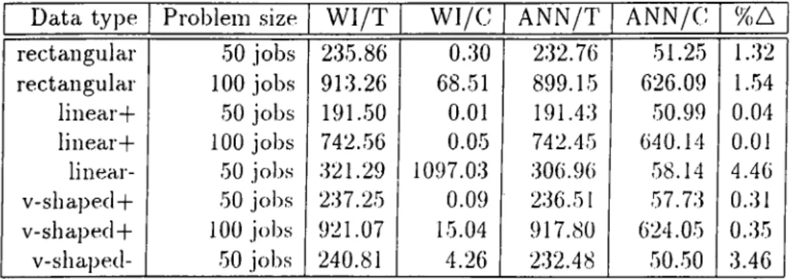
CHA PTER 4. THE PROPOSED PPROA Cl I 29 Table 4.1: Results of W1 and the proposed network ioi· single machine mean
Data type Problem size W I/T W I/C ANN/T ANN/C %A rectangular 50 jobs 235.86 0.30 232.76 51.25 1.32 rectangular 100 jobs 913.26 68.51 899.15 626.09 1.54 linear+ 50 jobs 191.50 0.01 191.43 50.99 0.04 linear+ 100 jobs 742.56 0.05 742.45 640.14 0.01 linear- 50 jobs 321.29 1097.03 306.96 58.14 4.46 v-shapecl + 50 jobs 237.25 0.09 236.51 57.73 0.31 v-shaped + 100 jobs 921.07 15.04 917.80 624.05 0.35 V-shaped- 50 jobs 240.81 4.26 232.48 50.50 3.46
In all of the test problems, processing times of the jobs were generated randomly between 1 and 100. Due dates were also generated randomly with respect to the limits specified by TF’ and RDD.
Simulation tests were made for the problem sizes of 50 and 100 jobs. For each of the 5 data types, ]:>airs of TF and RDD values were taken from the following set : [0.1,0.3,0.5,0.7,0.9]; 10 random samples from each case were generated which resulted in total of 2x5x5x5x10=2500 problems (Table 4.1).
In table 4.1, W I/T and ANN/T stands for mean tardiness of WI and the propo.sed network, respectively. W I/C and ANN/C stands for computation times of Wl (in seconds) and the proposed network. %A stands for percentage improvement in tardiness of the proposed method over the Wl algorithm. The results are based on the average of 250 problems solved with various TF and RDD values. Detailed results are given in appendix A.
Even though all the 250 problems were attem])ted to be solved for each data ty]>e, in some experiments (especially for the problems of linear- and v- shaped data types) the Wl algorithm could not hnish execution in 18 days of SUN Spark 2+ processing time. Eventually, comparisons could not be made for these data types.
A Confidence Interval (Cl) approach was also used to determine whether the mean tardiness performance of the proposed method is significantly better than the WI algorithm.
CHAPrEU. 4. THE PROPOSED ÁPPROACH 30 RECTANGULAR LINEAR-y·' d=p ■y·
p
V-SHAPED-# # # d=p # # ■ 0' ■CHAPrER 4. THE PROPOSED APPROACH 31 Table 4.2: Confidence interval te.sts for the difference between W1 and the
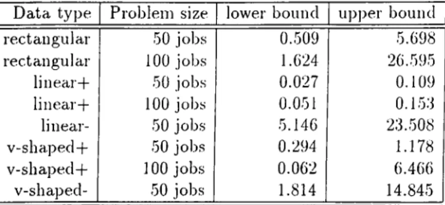
Data type Problem size lower bound upper bound rectangular 50 jobs 0.509 5.698 rectangular 100 jobs 1.624 26.595 linear-)- 50 jobs 0.027 0.109 linear-f 100 jobs 0.051 0.153 linear- 50 jobs 5.146 23.508 v-shaped-(- 50 jobs 0.294 1.178 v-shaped-f- 100 jobs 0.062 6.466 v-shaped- | 50 jobs 1.814 14.845
Table 4.3: Confidence interval test.s on the relative performance of the pro])osed network and W1 for .sizes 50 and 100 jobs:
Data type rectangular linear+ V -sh ap ed + lower bound -24.539 -0.105 -6.323 upper bound 2.528 0.037 1.267
As can be seen in Table 4.2, the mean dilference between the proj^osed method and the W1 algorithm was significant at cv = 0.05 (in the favor of the pro])osed method).
Further investigation was also made to determine whether the ])roblem size (i.e., the number of jobs) alTects the relative performance of the ])roposed method and the W1 algorithm. As depicted in Table 4.3, results of experi ments and confidence interval tests indicated that problem size did not affect the quality of solutions and the differences in performances of the proposed method and the WI algorithm.
A confidence interval test w'as made for varying tf and rdd values. For each case the proposed method performs significantly better than the WI algorithm. Especially the relative performance of the algorithms becomes more significant for tf values close to one (Table 4.4) or for rdd values close to zero (Table 4.5). When the tf values are close to zero or rdd values are close to one the relative performances of the algorithms are very close to each other.
The average computational time of the WI algorithm is significantly less than the ])ropo.sed algorithm for tf values less than 0.5 or rdd values greater than 0.5.
CHAPTER 4. THE PROPOSED APPROACH 32 Table 4.4: Confidence interval tests on the varying tf values lor the proposed network and WI for sizes 50 and 100 jobs:
TF lower bound upj)er bound 0.1 0.060 0.494 0.3 0.233 5.138 0.5 2.015 13.458 0.7 4.037 20.393 0.9 1.077 8.145
Table 4.5: Confidence interval tests on the varying rdd values for the ]>roposed network and WI for sizes 50 and 100 jobs:
RDD 0.1 0.3 0.5 0.7 0.9 lower bound 10.292 1.929 0.602 0.260 0.072 u]>]>er l)ound 29.201 7.713 2.772 1.151 1.058
In conclusion, the proposed network model was more successful than the WI algorithm especially for linear- and v-sha]:)ed- data. Moreover, the comjiu- tational requirements of WI increased enormously as tlie size of the problem increased for these data tyjjes. For the other data ty])es, the com])utational requirements of WI were extremely low but.
The complexity of the proposed method is {TF RDD)xiFlog{n) and it is not dependent on the data type. However, it was observed during the exper iments that the computational requirements of WI change dramatically with respect to different data types and at varying values of TF and RDD ])arame- ters.
In order to improve the performance of the ])roj)osed algorithm additional steps were also taken, such as incorporating simulated annealing and genetic algorithms during evolution of the network. Especially, Genetic Algorithms (GA) were seriously investigated. GA are search algorithms based on the me chanics of natural selection and natural genetics. They combine survival of the fittest among string structures with a structured yet randomized informa tion exchange to form a search algorithm with some innovative flair of human search. In every generation, a new set of artificial creatures (strings) is created