High resolution time frequency representation with significantly reduced cross-terms

A HIGH RESOLUTION TIME FREQUENCY REPRESENTATION WITH

SIGNIFICANTLY REDUCED CROSS-TERMS

A . Kemal Ozdemir and Orhan Arakan

Department

of

Electrical and Electronics Engineering,

Bilkent University, Ankara, TR-06533 TURKEY.

Phone

&

Fax: 90-312-2664307,

e-mail: kozdemir@ee.bilkent.edu.tr and oarikan@ee.bilkent.edu.tr

A B S T R A C T

A

novel algorithm is proposed for efficiently smoothing the slices of the Wigner distribution by exploiting the recently developed relation between the Radon transform of the am- biguity function and the fractional Fourier transformation

[ I ] . The main advantage of the new algorithm is its abil-

ity t o suppress cross-term interference on chirp-like auto- components without any detrimental effect to the auto- components. For a signal with N samples, the computa-

tional complexity of the algorithm is O ( N log N ) flops for

each smoothed slice of the Wigner distribution.

1. I N T R O D U C T I O N

Time-frequency representations have found important ap- plication areas in analysis, synthesis and detection of non stationary signals by revealing the signals joint time and frequency content

[a,

31. Much of the research in time- frequency signal processing has been devoted to design of new time-frequency representations. Among the represen- tations developed so far the Wigner distribution [4] has at- tracted much of the attention because of its nice theoretical properties including the preservation of the marginals and high auto-component concentration [ 2 , 51. The Wigner dis- tribution of a signal z ( t ) is given as

W z ( t , f ) = / z ( t

+

t ’ / 2 ) z * ( t - t’/2)e-32rtt’ dt’

,

( 1 )

where ( t , f ) denote the time and frequency coordinate. As it becomes clear from this definition, the Wigner distribution is a bilinear representation. Therefore the Wigner distri- bution of a multi-component signal z ( t ) =

xz,

z i ( t ) con- tains m(m- 1 ) / 2 cross terms of the form 2!&{WZiZj ( t ,

f)},

i

<

j , in addition to the auto-components W z i Z i ( t , f ) , where W Z t z j ( t , f ) is the cross WD [2, 31 of the signals zt.i(t) and z j ( t ) . The cross-terms usually interfere with the auto-components and decreases the interpreteability of the Wigner distribution. Thus the existence of cross-terms lim- its the use of the Wigner distribution in some practical ap- plications.

The cross-terms of the Wigner distribution have been extensively analyzed [6, 71. It has been found that the

cross terms lie at mid-time and mid-frequency of the auto- components, they are highly oscillatory and the frequency

0-7 803-6293-4/00/$10.00 02000

IEEE.

of oscillations increases with the increasing distance in time and frequency and they might have a peak value as high as

twice that of the auto-components. Based on these obser- vations it has been suggested that some sort of smoothing of the Wigner distribution is necessary to suppress the cross- terms a t the expense of broadening of the auto-components. In a unified framework, the representation obtained by low- pass filtering the Wigner distribution are studied under the name of Cohen’s bilinear class of shift invariant dis- tributions. In this class, the time-frequency representation

TF,(t, f ) of a signal z ( t ) is obtained as [2]

TF,(t,

f)

=

//

A,(v,

T ) ~ ( v , T)e-32r(ut+T’) d v d 7 1 ( 2 )

where

4(v,

T ) is the kernel of the distribution and &(v, T )

is the (symmetric) ambiguity function (AF) which is the

2-D inverse Fourier transform of the Wigner distribution:

The drawback of this class of distributions is that a fixed kernel can perform well only for a limited class of signals. On the other hand for a large class of signals, there is a trade-off between good cross-term suppression and high auto-component concentration. Therefore to obtain high- quality time-frequency representation, the kernel must be adapted to the characteristics of the input signal to obtain a data-adaptive smoothing. These considerations led to the development of Cohen’s class of time-frequency representa- tions with data-dependent kernels [2].

The basis of the recent research on the design of data- dependent kernels is the following observation: In the am- biguity plane, the auto-components lie around the origin and the cross-terms lie away from the origin [6]. Thus by designing a kernel

4(v,

7 ) which is apt to the characteristics

of the data in the ambiguity plane, higher quality represen- tations (more easily interpretable) are obtained (8, 91. The disadvantages of this approach are as follows: the obtained methods are computationally expensive, and kernel which is globally optimal does not necessarily produce locally op- timal results.

In this paper, a novel approach to design a new time- frequency representation is proposed. In contrast to the vast body of previous work, the proposed approach is based

on the Radon transform of the ambiguity function of the in- put signal, which is called as the Radon ambiguity function transform (RAFT) [l]. The proposed time-frequency rep- resentation cannot be described by either a fixed or signal dependent kernel, therefore it does not belong to Cohen’s class. However, by performing windowing on the resultant RAFT’S, it eliminates significant part of the cross-terms without reducing the auto-component concentration.

In Section 2 the mathematical details of the new approach are given, in Section 3 some simulation results are presented and finally in Section 4 conclusions are drawn.

The outline of the paper is as follows.

2. DIRECTIONAL SMOOTHING OF THE

WIGNER DISTRIBUTION

The most important drawback of the approaches based on the low-pass filtering of the WD is that, the low-pass filter is applied in all directions of the Wigner plane. Naturally this leads to broadening of the auto-components, because the auto-components may not have a low-pass characteris- tic along all orientations. For instance the slice of the WD of a linear chirp has a low-pass characteristic when the slice is along the chirp’s major axis, but is has significant high frequency content when the slice is lying along its minor axis as illustrated in Fig. 1 . Thus the directional smooth- ing of the WD by using low-pass filters with data-adaptive cut off frequencies appear t o be the natural solution to the problem. By this way the oscillatory cross-terms with sig- nificant high-frequency content are suppressed without es- sentially decreasing the auto-component concentration. At the end what we get is a high resolution timefrequency representation.

In this work, we assume that supports of the auto- components or the regions of the Wigner plane which are suspected to contain auto-components are specified before- hand. What has to be done is t o efficiently smooth the slices of these regions with data-adaptive low-pass filters. In the next subsection we develop a procedure t o efficiently smooth any arbitrarily chosen slice of the WD.

2.1. Directional smoothing algorithm

Suppose that we want to smooth the non-central slice of the Wigner distribution W, which passes through the point

( t o , fo) and makes an angle of

4

with the t i m e a x i s as shown

in Fig. 2 . I t is straightforward t o prove that this non- central slice of the Wigner distribution W, is the same as the central slice of the Wigner distribution of a signal y(t)

a t the same angle

4

(see Fig. 2 ) provided that the latter signal is defined in terms of the original one through the relation

y(t) = z ( t

+

to)e-32=’ot

.

₍₄₎

Thus we can formulate the smoothing problem in terms of the WD W,. By denoting the radial slice of the WD W, as SLC [W,](r,(p) E WY(rcos4,rsin(P), and impulse response of the real smoothing filter as h ( t ) , the directional smoothing can be mathematically expressed as

S ( T , 4 ) = h ( r )

;

SLC

[WYl(.,4)

,

(5)

where s ( r , 4 ) is the slice of the smoothed Wigner distribu- tion. By using the projection slice theorem [lo], the central slice of the Wigner distribution W, can be expressed as the Fourier transform of the Radon transform of the ambiguity function A,:

SLC

[W,](r,

4)

= / R D N [Ay](X,

4)2-32mrX

dX

,

(6)

where the Radon transform of the ambiguity function is defined as

R D N [Ay](X,

4)

= (A cos

4-

s sin

4,

X sin $+s cos

4)

d s .

(7) Thus (5) can be expressed in the (inverse) Fourier transform domain as

S(X,

4)

= H ( N R D N [AYl(X,

4) ,

(8)

where S(X,+) is the inverse Fourier transform of the slice s(r,

4)

with respect to the radial variable T , and H(X) is the inverse Fourier transform of the smoothing filter h ( t ) . This equation gives the basis of the algorithm for smoothing any slice of the Wigner distribution of a signal z ( t ) :

1. Compute the Radon transform R D N [A,](X,4) of the ambiguity function A,(v, T).

2. Design a multiplicative filter H(X) to capture the en- ergy around the origin and suppress the cross-terms away from the origin.

3. Apply the multiplicative filter H(X) t o the Radon transform R D N [A,](X,

4)

t o obtain S(X,

4).

4. Compute the slice

s ( r , 4 )

of the smoothed distribu-

tion from S(X,4) by using the Fourier transforma- tion.

This procedure can be repeated on different slices where adaptively chosen filters are utilized on each slice depend- ing on the auto-component location in the corresponding

R D N [Ay](&+). However t o have a practically useful al- gorithm, we have t o obtain the Radon transform of the ambiguity function efficiently. As we prove in Appendix A, the Radon transform of the ambiguity function A,(v, 7 ) can

be computed as

where a = 2 4 / ~ and z ( a - l ) ( t ) is the ( a - l) t h order frac-

tional Fourier transformation [Ill of the signal x ( t ) and in polar format ( d ,

4

+

~ / 2 ) is the closest point on the non- central slice of the WD t o the origin as shown in Fig. 2.

3. SIMULATION

In this section we investigate the performance of the pro- posed method in removing the cross-terms residing on the auto-components of the Wigner distribution. The synthetic test signal used in this simulation is generated by linearly combining 5 linear frequency modulated chirp signals with Gaussian envelopes. The intelligibility of the Wigner distri- bution of this multi-component signal is severely degraded

by the existence of cross-terms as seen in Fig. 3(a). In Fig. 3 (b), the Wigner distribution is computed on rectan- gular grids which contain supports of three of the auto- components. By using the new approach, these slices of the auto-components are smoothed by data-adaptive low-pass filtering and the obtained slices are plotted in Fig. 3 ( c ) . In Fig. 3 (d), the difference of the smoothed slices from the actual auto-components is shown to illustrate the high accuracy time-frequency representation provided by the al- gorithm.

In the next example we investigate the problem, where not only the interference terms but also one of the auto- components are superimposed on another auto-component. As shown.in Fig. 4(a), the Wigner distribution of the multi- component signal displays significant cross and auto-term noise on the chirp signal centered at the origin. In Fig. 4(b),

the smoothed slices of the WD along this chirp signal are plotted. As it can be seen from this plot, the noise terms are greatly attenuated.

4. CONCLUSIONS

A fast algorithm is developed for smoothing slices of the Wigner distribution to suppress the oscillatory cross-term components yielding a highly accurate representation of the auto-terms of the Wigner distribution. The new algorithm, which is especially tailored for but not limited to chirp-like components, is based on the recently established relation- ship between the Radon ambiguity function transform and fractional Fourier transform. In contrast to the smooth- ing algorithms which work by applying a low pass filter globally t o the WD, the new algorithm works locally on the slices of the WD. As shown by simulation examples, the proposed algorithm avoids the usual trade-off between cross-term suppression and auto-term broadening by tak- ing into account the characteristics of the cross-terms on the WD slices.

5. REFERENCES

[l] A. K. Ozdemir and 0. Arikan, “Efficient computation of the ambiguity function and the Wigner distribution on arbitrary line segments,” accepted for publication in IEEE Trans. Signal Process., Nov. 1999.

[ 2 ] L. Cohen, “Time-frequency distributions - A review,”

Proc. IEEE, vol. 77, pp. 941-981, July 1989.

[3] F. Hlawatsch and G. F. Boudreaux-Bartels, “Linear and quadratic time-frequency signal representations,”

IEEE Signal Processing Magazine, vol. 9, pp. 21-67, Apr. 1992.

[4] T. A. C. M. Claasen and W. F. G. Mecklenbrauker, “The Wigner distribution - A tool for time-time fre-

quency signal analysis, Part I: Continuous-time sig- nals,” Philips J . Res., vol. 35, no. 3, pp. 217-250, 1980. [5] T. A. C. M. Claasen and W. F. G. Mecklenbrauker, “The Wigner distribution - A tool for time-time

frequency signal analysis, Part 111: Rrelations with other time-frequency signal transformations,” Philips J . Res., vol. 35, no. 6, pp. 372-389, 1980.

[6] P. Flandrin, “Some features of time-frequency rep- resentations of multicomponent signals,” PTOC. IEEE Int. Conf. Acoust. Speech Signal Process., vol. 3,

[7] F. Hlawatsch, “Interference terms in the Wigner dis- tribution,” in Digital Signal Processing-84 (V. Cap- pellini and A. G. Constantidies, eds.), pp. 363-367, B. V. North Holland: Elsevier-Science Publishers, 1984.

[8] B. Ristic and B. Boashash, “Kernel design for time- frequency signal analysis using the Radon transform,”

IEEE Trans. Signal Process., vol. 41, pp. 1996-2008, May 1993.

[9] R.

G.

Baraniuk and D. L. Jones,

“A

signal-dependent time-frequency representation: Optimal kernel de- sign,” IEEE Trans. Signal Process., vol. 41, pp. 1589- 1601, Apr. 1993.

[lo]

R.

N. Bracewell, Two-dimensional imaging. Prentice-

Hall, 1995.

[Ill H. M. Ozaktas, M.

A.

Kutay, and D. Mendlovic, In- troduction t o the fractional Fourier transform and its applications, vol. 106, pp. 239-291. San Diego, Cali- fornia: Academic Press, 1999.

[12] L. B. Almedia, “The fractional Fourier transform and time-frequency representations,” IEEE Trans. Signal

[13] H. M. Ozaktas, 0. Arikan, M. A. Kutay, and

G. Bozdagi, “Digital computation of the fractional Fourier transform,” IEEE Trans. Signal Process.,

vol. 44, pp. 2141-2150, Sept. 1996. pp. 41B.4.1-41B.4.4, 1984.

Process., vol. 42, pp. 3084-3091, NOV. 1994.

A. THE RADON AMBIGUITY FUNCTION TRANSFORMATION

In [l], it has been shown that the Radon transform of the ambiguity function Ay(v, T), can be computed as

R D N [A,I(X,4) = Y ( a - l ) ( W Y & - l ) ( - W )

,

(10) where a = Z+/T and y(a-l) is the ( a - l)th order fractional Fourier transformation (FrFT) of the signal y ( t ) . To express the RAFT of y ( t ) in terms of the input signal z ( t ) , we first obtain the FrFT of y ( t ) by using the basic properties of the FrFT [12]:

(11) where p ( t ) = 27rt(fo sin

4

+

to cos

4 )

is the linear phase fac- tor and C = ezp(yr cos

4(f:

sin

4

+

t%

cos

4

+

f o t o sin

4 ) )

is a unit magnitude complex constant. Since we have the freedom to choose ( t o , f o ) as any point which lies on the line

LMT,

shown in Fig. 2 , we use this freedom to sim- plify the expression for the FrFT of y ( t ) . By choosing

( t o , f o ) (-dcos4,dsin$) as the closest point on Lw, to the origin (see Fig. 2 ) we simplify (11) as

~ ( ~ - ~ ) ( t ) = Ce”(t)z(a-l)(t - t o s i n +

+

f 0 c o s 4 )

,

Y ( a - l ) ( t ) = C”(a-l)(t -

4

’ (12)

Finally by substituting this relation into ( l o ) , we obtain the desired expression for the R.AFT of y ( t ) :

B. THE MODIFIED FAST FRACTIONAL FOURIER TRANSFORM ALGORITHM To simulate the proposed method, we need a fast algorithm to compute the samples of

~ ( ~ - ~ ) ( t

+ d ) . By using the algo-

rithm given in this appendix, the required samples can be computed in O ( N log N ) flops by using N uniformly spaced

samples of

z ( t ) .

This algorithm is obtained by modifying the algorithm in [13] to incorporate the delay term d , and removing the condition that the time-bandwidth product of z ( t ) be integer.

The Fast Fractional Fourier Transform Algorithm

Given z(n/A,), - N / 2

5

n

5

N / 2 - 1, to compute

za(mA,/(2N)

+

d),

-N

5

m

5

N

- 1. I t is assumed

that z ( t ) is scaled before obtaining its samples so that its WD is confined into a circle with diameter A,

5

fi

~ 3 1 .

Steps of the algorithm:

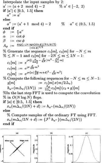
Interpolate the input samples by 2:

if la'l E [0.5, 1.51 then else

end if

a' := ( a

+

2 mod 4) - 2 % a' E [-2, 2)

a'' := a'

a'' := (a'

+

1 mod 4) - 2 % a'' E (0.5, 1.5)

4

:= Ea''

a := c o t 4

p

:= csc4

A+ := e x p ( - - j x sgn(sin + ) / 4 + j + / 2 )

% Generate the sequence cl[m], c3[m] for -N

5

m

%

5

N - 1 and cz[m] for -2N

5

m

5

2N - 1: I sin+1'/2 e 2 c g [ m ] := e J A 4 N m c3[m] := e J " b ( $ $ - m + + & 4 h,t,(mAz/(2N)) := &c3[m] (c2

*

g)[m]

% Compute the following sequences for -N

5

m

5

N-1: 9 [ml := ~1 [m] z(m/2A,)

%In the last step FFT is used t o compute the convolution

% in O(N1ogN) flops.

if ( a ( E [0.5, 1.51 then else

za(mA,/(2N)

+

d ) := hat! (mA,/(2N))

% Compute samples of the ordinary FT using FFT.

za(mA,/2N

+

d ) := {.F1 h , , i } ( m A Z / ( 2 N ) )

end if

Figure 1: A chirp signal has a low-pass characteristic along its major axis (b), and it has considerable bandwidth in along its minor axis (c).

t t

Figure 2: The non-central (left) and central (right) slices of the Wigner distribution W z ( t , f ) and W,(t, f ) .

Figure 3: The Wigner distribution (a), slices of the Wigner distribution (b), slices of the Wigner distribution smoothed with data-adaptive directional filtering (c), the difference of the smoothed slices from the auto-components only.

Figure 4: The Wigner distribution (a), smoothed slices of the Wigner distribution along one of the auto-components (b).