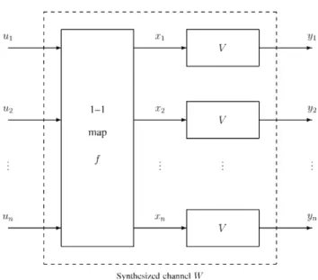
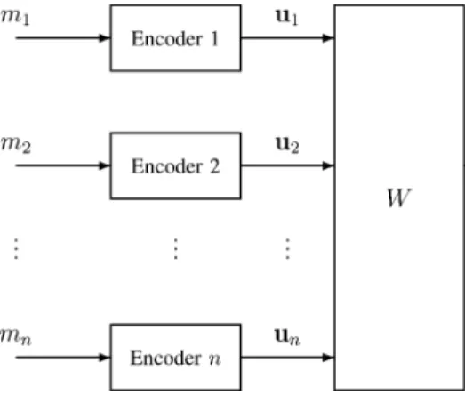
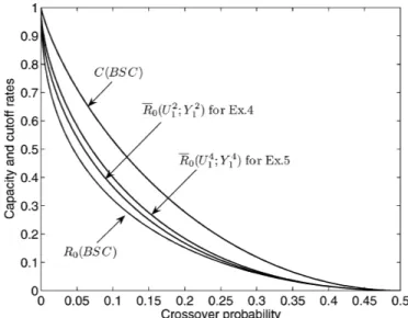
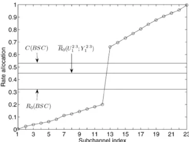
Channel combining and splitting for cutoff rate improvement

The Wisconsin K-12 Energy Education Pro- gram continues using formative assessments to help improve its services to teachers and to address stakeholder interests.. With the goal in

In addition to the case of pure states, we have shown that the Wigner–Yanase skew information (WYSI) can provide a reasonable estimation of the total amount of specific

As a particular example, we examine the system of two identical two-level atoms, interacting with a single cavity photon and show that the maximum entangled atomic states of the

We show that q-responsive choice rules require the maximal number of priority orderings in their smallest size MC representati- ons among all q-acceptant and path independent

Keywords: System identification, legged locomotion, mathematical models, spring-loaded inverted pendulum (SLIP) model, linear time periodic systems, harmonic transfer

Keywords: Reengineering, Operations Improvement, Manufacturing Productivity, Factory, Assembly, Machining, Material Handling, Changeover/Setup, Focused Factory,

It consists of some important stages such as taking the image of blood smear in which the white blood cells were painted, passing it through a couple of image enhancement

This is due to the fact that the encryption attacks on the IDEA versions with more than 3 rounds provide more than half of the 128 key bits with a complexity of between 2 73 –2