A Generative Model Based Adversarial Security of Deep Learning and Linear
Classifier Models
Samed Sivaslioglu
Tubitak Bilgem, Kocaeli, Turkey E-mail: [email protected] Ferhat Ozgur Catak
Simula Research Laboratory, Fornebu, Norway E-mail: [email protected]
Kevser ¸Sahinba¸s
Department of Management Information System, Istanbul Medipol University, Istanbul, Turkey E-mail: [email protected]
Keywords: adversarial machine learning, generative models, autoencoders Received: July 13, 2020
In recent years, machine learning algorithms have been applied widely in various fields such as health, transportation, and the autonomous car. With the rapid developments of deep learning techniques, it is critical to take the security concern into account for the application of the algorithms. While machine learning offers significant advantages in terms of the application of algorithms, the issue of security is ignored. Since it has many applications in the real world, security is a vital part of the algorithms. In this paper, we have proposed a mitigation method for adversarial attacks against machine learning models with an autoencoder model that is one of the generative ones. The main idea behind adversarial attacks against machine learning models is to produce erroneous results by manipulating trained models. We have also presented the performance of autoencoder models to various attack methods from deep neural networks to traditional algorithms by using different methods such as non-targeted and targeted attacks to multi-class logistic regression, a fast gradient sign method, a targeted fast gradient sign method and a basic iterative method attack to neural networks for the MNIST dataset.
Povzetek: S pomoˇcjo globokega uˇcenja je analizirana varnost pri sistemih strojnega uˇcenja.
1
Introduction
With the help of artificial intelligence technology, machine learning has been widely used in classification, decision making, voice and face recognition, games, financial as-sessment, and other fields [9, 12, 44, 45, 48]. The machine learning methods consider player’s choices in the anima-tion industry for games and analyze diseases to contribute to the decision-making mechanism [2, 6, 7, 15, 34, 46]. With the successful implementations of machine learning, attacks on the machine learning process and counter-attack methods and incrementing robustness of learning have be-come hot research topics in recent years [24, 27, 31, 37, 51]. The presence of negative data samples or an attack on the model can lead to producing incorrect results in the pre-dictions and classifications even in the advanced models.
It is more challenging to recognize the attack because of using big data in machine learning applications com-pared to other cybersecurity fields. Therefore, it is essen-tial to create components for machine learning that are re-sistant to this type of attack. In contrast, recent works have conducted in this area and demonstrated that the resis-tance is not very robust to attacks [10, 11]. These methods
have shown success against a specific set of attack methods and have generally failed to provide complete and generic protection[43].
Machine learning models already used in functional forms could be vulnerable to these kinds of attacks. For instance, by putting some tiny stickers on the ground in a junction, researchers confirmed that they could provoke an autonomous car to make an unnatural decision and drive into the opposite lane [16]. In another study, the re-searchers have pointed out that making hidden modifica-tions to an input image can fool a medical imaging opera-tion into labelling a benign mole as malignant with 100% confidence [17].
Previous methods have shown success against a specific set of attack methods and have generally failed to provide complete and generic protection [14]. This field has been spreading rapidly, and, in this field, lots of dangers have at-tracted increasing attention from escaping the filters of un-wanted and phishing e-mails, to poisoning the sensor data of a car or aircraft that drives itself [4, 41]. Disaster sce-narios can occur if any precautions are not taken in these systems [30].
The main contribution of this work is to explore the au-toencoder based generative models against adversarial ma-chine learning attacks to the models. Adversarial Mama-chine Learning has been used to study these attacks and reduce their effects [8, 32]. Previous works point out the funda-mental equilibrium to design the algorithms and to cre-ate new algorithms and methods that are resistant and ro-bust against attacks that will negatively affect this balance. However, most of these works have been implemented suc-cessfully for specific situations. In Section 3, we present some applications of these works.
This work aims to propose a method that not only presents a generic resistance to specific attack methods but also provides robustness to machine learning models in general. Our goal is to find an effective method that can be used by model trainers. For this purpose, we have pro-cessed the data with autoencoder before reaching to the ma-chine learning model.
We have used non-targeted and targeted attacks to mul-ticlass logistic regression machine learning models for ob-serving the change and difference between attack methods as well as various attack methods to neural networks such as fast gradient sign method (FGSM), targeted fast gradient sign method (T-FGSM) and basic iterative method (BIM). We have selected MNIST dataset that consists of numbers from people’s handwriting to provide people to understand and see changes in the data. In our previous works [3, 38], we applied the generative models both for data and model poisoning attacks with limited datasets.
The study is organized as follows. In Section 2, we first present the related works. In Section 3, we introduce several adversarial attack types, environments, and autoen-coder. In Section 4, we present selection of autoencoder model, activation function and tuning parameters. In Sec-tion 5, we provide some observaSec-tion on the robustness of autoencoder for adversarial machine learning with differ-ent machine learning algorithms and models. In Section 8, we conclude this study.
2
Related Work
In recent years, with the increase of the machine learning attacks, various studies have been proposed to create de-fensive measures against these attacks. Data sterility and learning endurance are recommended as countermeasures in defining a machine learning process [32]. They provide a model for classifying attacks against online machine learn-ing algorithms. Most of the studies in these fields have been focused on specific adversarial attacks and generally, presented the theoretical discussion of adversarial machine learning area [23, 25].
Bo Li and Yevgeniy Vorobeychik present binary do-mains and classifications. In their work, the approach starts with mixed-integer linear programming (MILP) with con-straint generation and gives suggestions on top of this. They also use the Stackelberg game multi-adversary model
algorithm and the other algorithm that feeds back the gen-erated adversarial examples to the training model, which is called as RAD (Retraining with Adversarial Examples) [28]. Their approach can scale thousands of features with RAD that showed robustness to several model erroneous specifications. On the other hand, their work is particular and works only in specific methods, even though it is pre-sented as a general protection method. They have proposed a method that implements successful results. Similarly, Xiao et al. provide a method to increase the speed of resis-tance training against the rectified linear unit (RELU) [36]. They provide that optimizing weight sparseness enables us to turn computationally demanding validation problems into solvable problems. They showed that improving ReLU stability leads to 4-13x faster validation times. They use weight sparsity and RELU stability for robust verification. It can be said that their methodology does not provide a general approach.
Yu et al. propose a study that can evaluate the neural network’s features under hostile attacks. In their study, the connection between the input space and hostile examples is presented. Also, the connection between the network strength and the decision surface geometry as an indicator of the hostile strength of the neural network is shown. By extending the loss surface to decision surface and other var-ious methods, they provide adversarial robustness by deci-sion surface. The geometry of the decideci-sion surface can-not be demonstrated most of the time, and there is no ex-plicit decision boundary between correct or wrong predic-tion. Robustness can be increased by constructing a good model, but it can change with attack intensity [50]. Their method can increase network’s intrinsic adversarial robust-ness against several adversarial attacks without involving adversarial training.
Mardy et al. investigate artificial neural networks resis-tant with adversity and increase accuracy rates with differ-ent methods, mainly with optimization and prove that there can be more robust machine learning models [43].
Pinto et al. provide a method to solve this problem with the supported learning method. In their study, they formu-late learning as a zero-sum, minimax objective function. They present machine learning models that are more resis-tant to disturbances are hard to model during the training and are better affected by changes in training and test con-ditions. They generalize reinforced learning on machine learning models. They propose a "Robust Adversarial Re-inforced Learning" (RARL), where they train an agent to operate in the presence of a destabilizing adversary that applies disturbance forces to the system. They presented that their method increased training stability, was robust to differences in training and testing conditions, and out-performed basically even in the absence of the adversary. However, in their work, Robust Adversarial Reinforced Learning may overfit itself, and sometimes it can miss pre-dicting without any adversarial being in presence [39].
Carlini and Wagner propose a model that the self-logic and the strength of the machine learning model with a
strong attack can be affected. They prove that these types of attacks can often be used to evaluate the effectiveness of potential defenses. They propose defensive distillation as a general-purpose procedure to increase robustness [11].
Harding et al. similarly investigate the effects of hostile samples produced from targeted and non-targeted attacks in decision making. They observed that non-targeted samples interfered more with human perception and classification decisions than targeted samples [22].
Bai et al. present a convolutional autoencoder model with the adversarial decoders to automate the generation of adversarial samples. They produce adversary examples by a convolutional autoencoder model. They use pooling com-putations and sampling tricks to achieve these results. After this process, an adversarial decoder automates the genera-tion of adversarial samples. Adversarial sampling is useful, but it cannot provide adversarial robustness on its own, and sampling tricks are too specific [5]. They gain a net perfor-mance improvement over the normal CNN.
Sahay et al. propose FGSM attack and use an autoen-coder to denoise the test data. They have also used an au-toencoder to denoise the test data, which is trained with both corrupted and healthy data. Then they reduce the dimension of the denoised data. These autoencoders are specifically designed to compress data effectively and re-duce dimensions. Hence, it may not be wholly generalized, and training with corrupted data requires a lot of adjust-ments to get better test results [33]. Their model provide that when test data is preprocessed using this cascading, the tested deep neural network classifier provides much higher accuracy, thus mitigating the effect of the adversarial per-turbation.
I-Ting Chen et al. also provide with FGSM attack on denoising autoencoders. They analyze the attacks from the perspective that attacks can be applied stealthily. They use autoencoders to filter data before applied to the model and compare it with the model without an autoencoder filter. They use autoencoders mainly focused on the stealth aspect of these attacks and used them specifically against FGSM with specific parameters [13]. They enhance the classifica-tion accuracy from 2.92% to 75.52% for the neural network classifier on the 10 digits and from 4.12% to 93.57% for the logistic regression classifier on digit 3s and 7s.
Gondim-Ribeiro et al. propose autoencoders attacks.
In their work, they attack 3 types of autoencoders: Sim-ple variational autoencoders, convolutional variational au-toencoders, and DRAW (Deep Recurrent AttentiveWriter). They propose to scheme an attack on autoencoders. As they accept that "No attack can both convincingly recon-struct the target while keeping the distortions on the input imperceptible.". They enable both DRAW’s recurrence and attention mechanism to lead to better resistance. Automatic encoders are recommended to compress data and more at-tention should be given to adversarial attacks on them. This method cannot be used to achieve robustness against adver-sarial attacks [40].
Table 2 shows the strength and the weakness of the each
paper.
3
Preliminaries
In this section, we consider attack types, data poisoning attacks, model attacks, attack environments, and autoen-coder.
3.1
Attack Types
Machine Learning attacks can be categorized into data poi-soning attacks and model attacks. The difference between the two attacks lies in the influencing type. Data poisoning attacks mainly focus on influencing the data, while model evasion attacks influencing the model for desired attack outcomes. Both attacks aim to disrupt the machine learning structure, evasion from filters, causing wrong predictions, misdirection, and other problems for the machine learning process. In this paper, we mainly focus on machine learn-ing model attacks.
3.1.1 Data Poisoning Attacks
According to machine learning methods, algorithms are trained and tested with datasets. Data poisoning in machine learning algorithms has a significant impact on a dataset and can cause problems for algorithm and confusion for developers. With poisoning the data, adversaries can com-promise the whole machine learning process. Hence, data poisoning can cause problems in machine learning algo-rithms.
3.1.2 Model Attacks
Machine learning model attacks have been applied mostly in adversarial attacks, and evasion attacks being have been used most extensively in this category. For spam emails, phishing attacks, and executing malware code, adversaries apply model evasion attacks. There are also some benefits to adversaries in misclassification and misdirection. In this type of attack, the attacker does not change training data but disrupts or changes its data and diverse this data from the training dataset or make this data seem safe. This study mainly concentrates on model attacks.
3.2
Attack Environments
There are two significant threat models for adversarial at-tacks: the white-box and black-box models.
3.2.1 White Box Attacks
Under the white-box setting, the internal structure, design, and application of the tested item are accessible to the ad-versaries. In this model, attacks are based on an analysis of the internal structure. It is also known as open box at-tacks. Programming knowledge and application knowledge
Table 1: Related Work Summary
Research Study Strength Weakness
Adversarial Machine Learning [32] Introduces the emerging field of Adversarial Machine Learn-ing.
Discusses the countermeasures against attacks without sug-gesting a method.
Evasion-Robust
Classification on Binary Domains [28]
Demonstrates some methods that can be used on Binary Do-mains, which are based on MILP.
Very specific about the robustness, even though it is presented as a general method.
Training for Faster Adversarial Robust-ness Verification via Inducing ReLU Stability [36]
Using weight sparsity and RELU stability for robust verifica-tion.
Does not provide a general approach, or universality as it is suggested in paper.
Interpreting Adversarial Robustness: A View from Decision Surface in Input Space [50]
By extending the loss surface to decision surface and other various methods, they provide adversarial robustness by de-cision surface.
The geometry of the decision surface cannot be shown most of the times and there is no explicit decision boundary be-tween correct or wrong prediction. Robustness can be in-creased by constructing a good model but it can change with attack intensity.
Robust Adversarial Reinforcement Learning [39]
They have tried to generalize reinforced learning on machine learning models. They suggested a Robust Adversarial Re-inforced Learning (RARL) where they have trained an agent to operate in the presence of a destabilizing adversary that applies disturbance forces to the system.
Robust Adversarial Reinforced Learning may overfit itself and sometimes it may mispredict without any adversarial be-ing in presence.
Alleviating Adversarial Attacks via Con-volutional Autoencoder [5]
They have produced adversary examples via a convolutional autoencoder model. Pooling computations and sampling tricks are used. Then an adversarial decoder automate the generation of adversarial samples.
Adversarial sampling is useful but it cannot provide adversar-ial robustness on its own. Sampling tricks are also too speci-fied.
Combatting Adversarial Attacks through Denoising and Dimensionality Reduc-tion: A Cascaded Autoencoder Ap-proach [33]
They have used an autoencoder to denoise the test data which is trained with both corrupted and normal data. Then they reduce the dimension of the denoised data.
Autoencoders specifically designed to compress data effec-tively and reduce dimensions. Therefore it may not be com-pletely generalized and training with corrupted data requires a lot of adjustments for test results.
A Comparative Study of Autoencoders against Adversarial Attacks [13]
They have used autoencoders to filter data before applying into the model and compare it with the model without au-toencoder filter.
They have used autoencoders mainly focused on the stealth aspect of these attacks and use them specifically against FGSM with specific parameters.
Adversarial Attacks on Variational Au-toencoders [40]
They propose a scheme to attack on autoencoders and validate experiments to three autoencoder models: Simple, convolu-tional and DRAW (Deep Recurrent Attentive Writer).
As they have accepted "No attack can both convincingly re-construct the target while keeping the distortions on the input imperceptible.". it cannot provide robustness against adver-sarial attacks.
Understanding Autoencoders with Infor-mation Theoretic Concepts [47]
They examine data processing inequality with stacked au-toencoders and two types of information planes with autoen-coders. They have analyzed DNNs learning from a joint geo-metric and information theoretic perspective, thus emphasiz-ing the role that pair-wise mutual information plays important role in understanding DNNs with autoencoders.
The accurate and tractable estimation of information quanti-ties from large data seems to be a problem due to Shannon’s definition and other information theories are hard to estimate, which severely limits its powers to analyze machine learning algorithms.
Adversarial Attacks and Defences Com-petition [42]
Google Brain organized NIPS 2017 to accelerate research on adversarial examples and robustness of machine learning classifiers. Alexey Kurakin and Ian Goodfellow et al. present some of the structure and organization of the competition and the solutions developed by several of the top-placing teams.
We experimented with the proposed methods of this compe-tition bu these methods do not provide a generalized solution for the robustness against adversarial machine learning model attacks.
Explaining And
Harnessing Adversarial Examples [19]
Ian Goodfellow et al. makes considerable observations about Gradient-based optimization and introduce FGSM.
Models may mislead for the efficiency of optimization. The paper focuses explicitly on identifying similar types of prob-lematic points in the model.
are essential. White-box tests provide a comprehensive as-sessment of both internal and external vulnerabilities and are the best choice for computational tests.
3.2.2 Black Box Attacks
In the black-box model, internal structure and software testing are secrets to the adversaries. It is also known as behavioral attacks. In these tests, the internal structure does not have to be known by the tester. They provide a comprehensive assessment of errors. Without changing the learning process, black box attacks provide changes to be observed as external effects on the learning process rather than changes in the learning algorithm. In this study, the main reason behind the selection of this method is the ob-servation of the learning process.
3.3
Autoencoder
INPUTS x1 x2 x3 xn-2 xn-1 xn ... Input Layer ... ... Hidden Layer I OUTPUTS ... ... ...Hidden Layer IV Output Layer Hidden Layer II Hidden Layer III
x1 x2 x3 xn-2 xn-1 xn Autoencoder
Figure 1: Autoencoder Layer Structure
An autoencoder neural network is an unsupervised learn-ing algorithm that takes inputs and sets target values to be equals of the input values [47]. Autoencoders are gener-ative models that apply backpropagation. They can work without the results of these inputs. While the use of a learning model is in the form of model.fit(X,Y), au-toencoders work as model.fit(X,X). The autoencoder works with the ID function to get the output x that cor-responds to x entries. The identity function seems to be a particularly insignificant function to try to learn; how-ever, there is an interesting structure related to the data, putting restrictions such as limiting the number of hid-den units on the network[47]. They are neural networks which work as neural networks with an input layer, hid-den layers and an output layer but instead of predicting Y as in model.fit(X,Y), they reconstruct X as in model.fit(X,X). Due to this reconstruction being un-supervised, autoencoders are unsupervised learning mod-els. This structure consists of an encoder and a decoder part. We will define the encoding transition as φ and de-coding transition as ψ.
φ : X → F ψ : F → X
φ, ψ = argminφ,ψ||X − (ψ ◦ φ)X||2
With one hidden layer, encoder will take the input x ∈
Rd = χ and map it to h ∈ Rp = F . The h below is
re-ferred to as latent variables. σ is an activation function such
as ReLU or sigmoid which were used in this study[1, 20]. b is bias vector, W is weight matrix which both are usu-ally initialized randomly then updated iteratively through training[35].
h = σ(W x + b)
After the encoder transition is completed, decoder
tran-sition maps h to reconstruct x0.
x0 = σ0(W0h + b0) where σ0, W0, b0 of decoder are
unrelated to σ, W , b of encoder. Loss of autoencoders are trained to be minimal, showed as L below.
L(x, x0) = ||x−x0||2= ||x−σ0(W0(σ(W x+b))+b0)||2
So the loss function shows the reconstruction errors, which need to be minimal. After some iterations with input training set x is averaged.
In conclusion, autoencoders can be seen as neural net-works that reconstruct inputs instead of predicting them. In this paper, we will use them to reconstruct our dataset inputs.
4
System Model
This section presents the selection of autoencoder model, activation function, and tuning parameters.
4.1
Creating Autoencoder Model
In this paper, we have selected the MNIST dataset to ob-serve changes easily. Therefore, the size of the layer struc-ture in the autoencoder model is selected as 28 and mul-tipliers to match the MNIST datasets, which represents the numbers by 28 to 28 matrixes. Figure 2 presents the
structure of matrixes. The modified MNIST data with
autoencoder is presented in Figure 3. In the training of the model, the encoded data is used instead of using the MNIST datasets directly. As a training method, a multi-class logistic regression method is selected, and attacks are applied to this model. We train autoencoder for 35 epochs. Figure 4 provides the process diagram.
INPUTS x1 x2 x3 x782 x783 x784 ... 784 Relu ... ... 504 Relu OUTPUTS ... ... ... 504 Exponential 784 Softplus 28 Relu 28 Relu x1 x2 x3 x782 x783 x784 Autoencoder Decoding Encoding
Figure 2: Autoencoder Activation Functions. Note that layer sizes given according to the dataset which is MNIST dataset
4.2
Activation Function Selection
In machine learning and deep learning algorithms, the ac-tivation function is used for the computations between
Figure 3: Normal and Encoded Data Set of MNIST
Data Set Autoencoder
Attack Results Untargeted and Targeted Attacks on Trained Model Encoded Data Set Model Training
Figure 4: Process Diagram
0 5 10 15 20 25 30 35 Epoch 600 620 640 660 680 700 Lo ss Relu Train Test
(a) Relu Loss History
0 5 10 15 20 25 30 35 Epoch 560 570 580 590 600 Lo ss Sigmoid Train Test
(b) Sigmoid Loss History
0 5 10 15 20 25 30 35 Epoch 800 850 900 950 1000 1050 1100 Lo ss Softsign Train Test
(c) Softsign Loss History
0 5 10 15 20 25 30 35 Epoch 600 700 800 900 1000 1100 1200 Lo ss Tanh Train Test
(d) Tanh Loss History
Figure 5: Loss histories of different activation functions
hidden and output layers[18]. The loss values are com-pared with different activation functions. Figure 5 indi-cates the comparison results of loss value. Sigmoid and
ReLUhave the best performance among these values and
gave the best results. Sigmoid has more losses at lower epochs than ReLU, but it has better results. Therefore, it is aimed to reach the best result of activation function in both layers. The model with the least loss value is to make the coding parts with the ReLU function and to use the
exponentialand softplus functions in the analysis
part respectively. These functions are used in our study. Figure 6 illustrates the result of the loss function, and Fig-ure 2 presents the structFig-ure of the model with the activation functions.
4.3
Tuning Parameters
The tuning parameters for autoencoders depend on the dataset we use and what we try to apply. As previously mentioned, ReLU and sigmoid function are selected to be activation function for our model [1, 18]. ReLU is the ac-tivation function through the whole autoencoder while ex-ponential is the softplus being the output layer’s activation function which yields the minimal loss. Figure 2 presents
0 5 10 15 20 25 30 35 Epoch 520 530 540 550 560 570 580 590 Lo ss Optimized Train Test
Figure 6: Optimized Relu Loss History
the input size as 784 due to our dataset and MNIST dataset contains 28x28 pixel images[29]. Encoding part for our autoencoder size is 784 × 504 × 28 and decoding size is 28 × 504 × 784.
This structure is selected by the various neural network structures that take the square of the size of the matrix, lower it, and give it to its dimension size lastly. The last hidden layer of the decoding part with the size of 504 uses exponential activation function, and an output layer with the size of 784 uses softplus activation func-tion [14, 21]. We used adam optimizer with categorical crossentropy[26, 49]. We see that a small number is enough for training, so we select epoch number for autoencoder as 35. This is the best epoch value to get meaningful results for both models with autoencoder and without autoencoder to see accuracy. In lower values, models get their accu-racy scores too low for us to see the difference between them, even though some models are structurally stronger than others.
5
Experiments with MNIST Dataset
5.1
Introduction
We examine the robustness of autoencoder for adversar-ial machine learning with different machine learning algo-rithms and models to see that autoencoding can be a gener-alized solution and an easy to use defense mechanism for most adversarial attacks. We use various linear machine learning model algorithms and neural network model algo-rithms against adversarial attacks.
5.2
Autoencoding
In this section, we look at the robustness provided with auto-encoding. We select a linear model and a neural net-work model to demonstrate this effectiveness. In these models, we also observe the robustness of different attack methods. We also use the MNIST dataset for these exam-ples.
5.2.1 Multi-Class Logistic Regression
In linear machine learning model algorithms, we use mainly two attack methods: Non-Targeted and Targeted Attacks. The non-targeted attack does not concern with how the machine learning model makes its predictions and
Predicted Values 0 1 2 3 4 5 6 7 8 9 Actual Values 0 973 0 4 0 1 2 9 1 4 6 1 0 1127 3 0 0 0 3 5 1 2 2 2 6 1016 4 3 0 2 10 4 1 3 0 0 2 1002 0 10 0 5 3 4 4 0 0 3 0 966 0 1 0 0 8 5 0 0 0 1 0 869 3 0 1 2 6 1 1 0 0 1 5 938 0 1 0 7 1 0 4 0 1 1 0 999 3 9 8 3 1 0 3 2 3 1 2 953 3 9 0 0 0 0 8 2 1 6 4 974
Figure 7: Confusion matrix of the model without any attack and without autoencoder
tries to force the machine learning model into mispredic-tion. On the other hand, targeted attacks focus on lead-ing some correct predictions into mispredictions. We have three methods for targeted attacks: Natural, Non-Natural, and one selected target. Firstly, natural targets are derived from the most common mispredictions made by the ma-chine learning model. For example, guessing number 5 as 8, and number 7 as 1 are common mispredictions. Nat-ural targets take these non-targeted attack results into ac-count and attack directly to these most common mispredic-tions. So, when number 5 is seen, an attack would try to make it guessed as number 8. Secondly, non-natural tar-geted attacks are the opposite of natural tartar-geted attacks. It takes the minimum number of mispredictions made by the machine learning model with the feedback provided by non-natural attacks. For example, if number 1 is least mispredicted as 0, the non-natural target for number 1 is 0. Therefore, we can see that how much the attack affects the machine learning model beyond its common mispredic-tions. Lastly, one targeted attack focuses on some random numbers. The aim is to make the machine learning model mispredict the same number for all numbers. For linear classifications, we select multi-class logistic regression to analyze the attacks. Because we do not interact with these linear classification algorithms aside from calling their de-fined functions from scikit-learn library, we use a black-box environment for these attacks. In our study, the attack method against multi-class classification models developed in NIPS 2017 is used [42]. An epsilon value is used to de-termine the severity of the attack, which we select 50 in this study to demonstrate the results better. We apply a non-targeted attack to a multi-class logistic regression trained model which is trained with MNIST dataset without an au-toencoder. The confusion matrix of this attack is presented in 9.
The findings from Figure 9 and 10 show that an autoen-coder model provides robustness against non-targeted at-tacks. The accuracy value change with epsilon is presented in Figure 13. Figure 11 illustrates the change and perturba-tion of the selected attack with epsilon value as 50.
We apply a non-targeted attack on the multi-class logis-tic regression model with autoencoder and without autoen-coder. Figure 13 provides a difference in accuracy metric. The detailed graph of the non-targeted attack on the model
Predicted Values 0 1 2 3 4 5 6 7 8 9 Actual Values 0 973 0 4 0 1 2 9 1 4 6 1 0 1127 3 0 0 0 3 5 1 2 2 2 6 1016 4 3 0 2 10 4 1 3 0 0 2 1002 0 10 0 5 3 4 4 0 0 3 0 966 0 1 0 0 8 5 0 0 0 1 0 869 3 0 1 2 6 1 1 0 0 1 5 938 0 1 0 7 1 0 4 0 1 1 0 999 3 9 8 3 1 0 3 2 3 1 2 953 3 9 0 0 0 0 8 2 1 6 4 974
Figure 8: Confusion matrix of the model without any attack and with autoencoder
Predicted Values 0 1 2 3 4 5 6 7 8 9 Actual Values 0 247 0 17 51 8 73 32 20 8 7 1 0 0 34 8 0 8 0 15 30 13 2 32 18 69 37 181 24 251 288 191 255 3 49 174 222 8 128 106 25 193 489 141 4 4 0 34 49 14 57 59 29 10 231 5 509 58 56 154 43 9 502 110 55 172 6 45 0 93 35 68 109 4 5 25 1 7 23 210 48 22 33 26 43 26 52 1 8 51 678 366 586 31 378 23 141 0 189 9 47 13 60 76 469 60 25 194 137 0
Figure 9: Confusion matrix of non-targeted attack to model without autoencoder Predicted Values 0 1 2 3 4 5 6 7 8 9 Actual Values 0 987 0 7 8 0 13 0 1 5 4 1 0 1137 8 0 1 1 0 4 4 5 2 0 0 958 2 4 2 0 15 0 0 3 0 0 9 886 3 52 1 3 13 9 4 0 0 3 4 923 11 0 10 1 28 5 0 0 0 24 1 643 0 0 0 0 6 5 0 5 2 3 28 962 2 2 0 7 0 0 7 0 1 1 0 932 5 4 8 2 5 31 72 1 116 0 12 944 9 9 1 0 3 14 35 13 0 54 8 931
Figure 10: Confusion matrix of non-targeted attack to model with autoencoder
Figure 11: Value change and perturbation of a non-targeted attack on model without autoencoder
Figure 12: Value change and perturbation of a non-targeted attack on model with autoencoder
with autoencoder is presented in Figure 14. The changes in the MNIST dataset after autoencoder is provided in
Fig-ure 3. The value change and perturbation of an epsilon 50 value on data are indicated in Figure 12.
Figure 13: Comparison of accuracy with and without au-toencoder for non-targeted attack
Figure 14: Details of accuracy with autoencoder for non-targeted attack
The following process is presented in Figure 4. In the examples with the autoencoder, data is passed through the autoencoder and then given to the training model, in our current case a classification model with multi-class logistic regression. Multi-class logistic regression uses the encoded dataset for training. Figure 10 provides to see improvement as a confusion matrix. For the targeted attacks, we select three methods to use. The first one is natural targets for MNIST dataset, which is also defined in NIPS 2017 [42]. Natural targets take the non-targeted attack results into ac-count and attack directly to these most common mispre-dictions. For example, the natural target for number 3 is 8. When we apply the non-targeted attack, we obtain these results. Heat map for these numbers is indicated in Figure 77.
The second method of targeted attacks is non-natural tar-gets which is the opposite of natural tartar-gets. We select the least mis predicted numbers as the target. These numbers is indicated as the heat map in Figure 77. The third method is the selection one number and making all numbers predict it. We randomly choose 7 as that target number. Targets for these methods are presented in Figure 16. The confu-sion matrixes for these methods are presented below.
Figure 15: Heatmap of actual numbers and mispredictions
Natural Targets Actual NumbersTarget Numbers 06 18 28 83 94 85 06 97 38 94 Non-Natural Targets Actual NumbersTarget Numbers 01 10 20 13 14 15 16 67 08 96 One Number Targeted Actual NumbersTarget Numbers 07 17 27 73 74 75 76 77 78 97
Figure 16: Actual numbers and their target values for each targeted attack method
Predicted Values 0 1 2 3 4 5 6 7 8 9 Actual Values 0 291 0 10 9 1 5 10 16 1 1 1 0 0 1 0 0 0 0 2 0 0 2 1 7 70 14 3 1 10 806 25 27 3 6 10 46 45 7 38 6 17 786 9 4 9 6 11 10 84 11 13 23 8 920 5 680 3 22 21 5 49 559 15 29 0 6 1 0 40 3 8 8 329 2 1 0 7 0 0 4 1 6 1 3 18 3 0 8 18 1124 783 917 17 735 26 41 130 17 9 1 1 12 6 844 2 8 81 14 36
Figure 17: Confusion matrix of natural targeted attack to model without autoencoder
Predicted Values 0 1 2 3 4 5 6 7 8 9 Actual Values 0 989 0 2 1 0 6 7 1 0 1 1 0 1105 2 0 0 1 0 0 0 0 2 0 0 979 4 0 1 0 2 0 0 3 0 0 0 972 0 12 0 1 4 32 4 0 0 0 0 889 1 2 1 0 0 5 0 0 0 0 0 713 0 0 0 0 6 3 0 3 0 1 8 969 0 1 0 7 0 0 6 1 0 0 0 943 0 11 8 3 29 35 46 3 134 2 1 914 6 9 1 3 1 2 77 2 2 57 44 964
Figure 18: Confusion matrix of natural targeted attack to model with autoencoder
5.2.2 Neural Networks
We use neural networks with the same principles as multi-class logistic regressions and make attacks to the machine
Predicted Values 0 1 2 3 4 5 6 7 8 9 Actual Values 0 735 147 281 41 8 36 31 29 694 12 1 3 7 22 565 134 259 105 26 34 39 2 29 88 200 53 107 15 214 170 135 22 3 37 59 96 71 41 95 9 136 59 19 4 3 0 16 8 224 42 53 37 3 362 5 83 0 5 31 1 2 107 14 5 4 6 72 8 99 24 103 110 422 39 28 380 7 5 100 22 6 7 7 6 156 6 0 8 33 741 246 195 30 258 13 104 22 163 9 7 1 12 32 320 26 4 310 11 9
Figure 19: Confusion matrix of non-natural targeted at-tack to model without autoencoder
Predicted Values 0 1 2 3 4 5 6 7 8 9 Actual Values 0 994 0 1 0 0 7 0 0 0 0 1 0 1147 0 2 0 6 0 4 2 1 2 2 1 991 0 0 6 2 2 30 0 3 0 0 4 992 0 71 0 5 2 1 4 0 0 0 0 973 4 0 5 0 1 5 0 0 7 0 1 597 1 1 4 0 6 2 0 3 0 2 32 964 1 0 1 7 0 0 0 0 1 1 0 1001 0 0 8 3 1 5 5 0 170 1 5 917 8 9 0 0 1 3 0 8 0 6 0 992
Figure 20: Confusion matrix of non-natural targeted at-tack to model with autoencoder
Predicted Values 0 1 2 3 4 5 6 7 8 9 Actual Values 0 281 0 17 14 1 27 17 0 1 0 1 0 0 9 0 0 0 0 0 0 0 2 0 0 69 0 1 2 32 0 1 0 3 16 12 330 109 2 132 46 0 96 0 4 1 0 7 4 36 22 16 0 1 1 5 69 0 9 12 0 13 165 0 6 0 6 5 0 38 4 0 27 164 0 3 0 7 612 1114 372 778 828 406 479 1021 731 1005 8 6 25 116 61 0 139 21 0 28 0 9 17 0 32 44 107 82 24 0 130 4
Figure 21: Confusion matrix of one number targeted at-tack to model without autoencoder
Predicted Values 0 1 2 3 4 5 6 7 8 9 Actual Values 0 991 0 3 0 0 8 0 0 0 0 1 0 1139 7 0 0 1 0 0 3 0 2 0 0 955 0 0 0 0 0 0 0 3 0 0 20 991 0 33 1 0 7 0 4 1 0 4 0 947 4 1 0 1 1 5 0 0 0 0 0 775 0 0 0 0 6 0 0 5 0 0 11 960 0 0 0 7 2 3 20 18 25 2 1 1033 19 104 8 0 0 15 0 0 38 0 0 945 0 9 1 0 2 3 0 8 0 0 7 885
Figure 22: Confusion matrix of one number targeted at-tack to model with autoencoder
learning model. We use the same structure, layer, activation functions and epochs for these neural networks as we use in our autoencoder for simplicity. Although this robustness will work with other neural network structures, we will not demonstrate them in this study due to structure designs that can vary for all developers. We also compare the results of these attacks with both the data from the MNIST dataset
Figure 23: Comparison of accuracy with and without au-toencoder for targeted attacks. AE stands for the models with autoencoder, WO stands for models without autoen-coder
Figure 24: Details of accuracy with autoencoder for tar-geted attacks
and the encoded data results of the MNIST dataset. As for attack methods, we select three methods: FGSM, T-FGSM and BIM. Cleverhans library is used for providing these attack methods to the neural network, which is from the Keras library.
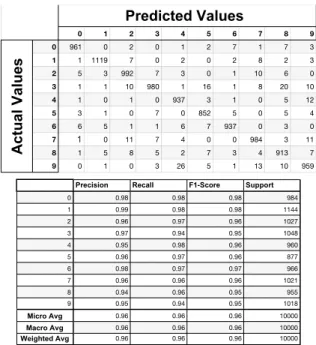
We examine the differences between the neural network model that has autoencoder and the neural network model that takes data directly from the MNIST dataset with confu-sion matrixes and classification reports. Firstly, our model without autoencoder gives the following results, as seen in Figure 25 for the confusion matrix and the classification report. The results with the autoencoder are presented in Figure 26. Note that these confusion matrixes and classifi-cation reports are indicated before any attack.
Fast Gradient Sign Method:
There is a slight difference between the neural network models with autoencoder and without autoencoder model. We apply the FGSM attack on both methods. The method uses the gradients of the loss accordingly for creating a new image that maximizes the loss. We can say the gradients are generated accordingly to input images. For these reasons, the FGSM causes a wide variety of models to misclassify their input [19].
As we expect due to results from multi-class logistic re-gression, autoencoder gives robustness to the neural net-work model too. After the DGSM, the neural netnet-work with-out an autoencoder suffers an immense drop in its accuracy,
Predicted Values 0 1 2 3 4 5 6 7 8 9 Actual Values 0 974 0 5 0 1 2 7 1 5 5 1 0 1125 4 0 0 0 3 4 0 2 2 0 1 1003 1 0 0 2 8 1 0 3 1 4 3 1004 0 7 0 2 0 1 4 0 0 3 0 970 0 7 0 3 14 5 0 0 0 1 0 873 4 0 1 2 6 1 2 0 0 4 5 930 0 0 0 7 2 0 8 0 1 2 0 1005 4 8 8 2 3 6 4 1 2 5 3 957 4 9 0 0 0 0 5 1 0 5 3 973
Precision Recall F1-Score Support
Micro Avg Macro Avg Weighted Avg
Figure 25: Confusion matrix and classification report of the neural network model without autoencoder
Predicted Values 0 1 2 3 4 5 6 7 8 9 Actual Values 0 966 0 4 0 0 2 3 0 3 3 1 0 1122 2 1 1 0 2 6 2 3 2 3 3 1013 7 3 0 2 13 2 2 3 0 0 3 982 0 5 0 8 7 2 4 0 0 1 1 954 1 7 0 4 6 5 1 2 0 10 0 874 4 1 5 6 6 4 4 1 1 2 5 937 0 2 0 7 1 1 4 3 8 2 0 990 2 8 8 3 3 3 3 3 2 3 2 945 7 9 2 0 1 2 11 1 0 8 2 972
Precision Recall F1-Score Support
Micro Avg Macro Avg Weighted Avg
Figure 26: Confusion matrix and classification report of the neural network model with autoencoder
and the FGSM works as intended. But the neural network model with autoencoder only suffers a 0.01 percent accu-racy drop.
Targeted Fast Gradient Sign Method: There is a di-rected type of FGSM, called T-FGSM. It uses the same
principles to maximize the loss of the target. In this
method, a gradient step is computed for giving the same misprediction for different inputs.
In the confusion matrix, the target value for this attack is number 5. The neural network model with the autoencoder is still at the accuracy of 0.98. The individual differences
Predicted Values 0 1 2 3 4 5 6 7 8 9 Actual Values 0 80 1 42 7 16 11 68 7 24 14 1 2 5 125 5 34 6 20 16 30 11 2 177 127 73 120 43 3 47 95 264 5 3 19 13 344 50 7 337 54 504 234 171 4 17 538 35 2 85 1 356 47 18 295 5 68 2 6 351 1 99 177 3 185 63 6 275 8 9 0 32 70 71 0 38 1 7 20 215 177 64 228 7 7 40 48 318 8 109 223 206 303 69 253 154 68 16 105 9 213 3 15 108 467 105 4 248 117 26
Precision Recall F1-Score Support
Micro Avg Macro Avg Weighted Avg
Figure 27: Confusion matrix and classification report of the neural network model without autoencoder after FGSM attack Predicted Values 0 1 2 3 4 5 6 7 8 9 Actual Values 0 966 0 5 0 0 2 2 1 3 2 1 0 1122 3 0 3 0 2 5 1 3 2 3 2 1009 8 4 0 2 11 2 3 3 0 0 4 980 0 5 0 9 7 2 4 0 1 1 1 956 2 8 1 4 8 5 1 2 0 11 0 872 3 1 7 5 6 4 4 1 1 2 5 939 0 2 0 7 1 2 4 3 5 2 0 988 2 8 8 3 2 4 4 2 3 2 2 942 8 9 2 0 1 2 10 1 0 10 4 970
Precision Recall F1-Score Support
Micro Avg Macro Avg Weighted Avg
Figure 28: Confusion matrix and classification report of the neural network model with autoencoder after FGSM attack
are presented when compare with Figure 26. Basic Iterative Method:
BIM is an extension of FGSM to apply it multiple times with iterations. It provides the recalculation of a gradient attack for each iteration.
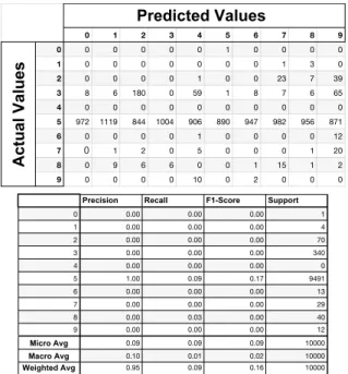
This is the most damaging attack for the neural net-work model that takes its inputs directly from the MNIST Dataset without an autoencoder. The findings from Fig-ure 31 show that the accuracy drops between 0.01 and 0.02 percent. The neural network model with autoencoder’s
ac-Predicted Values 0 1 2 3 4 5 6 7 8 9 Actual Values 0 0 0 0 0 0 1 0 0 0 0 1 0 0 0 0 0 0 0 1 3 0 2 0 0 0 0 1 0 0 23 7 39 3 8 6 180 0 59 1 8 7 6 65 4 0 0 0 0 0 0 0 0 0 0 5 972 1119 844 1004 906 890 947 982 956 871 6 0 0 0 0 1 0 0 0 0 12 7 0 1 2 0 5 0 0 0 1 20 8 0 9 6 6 0 0 1 15 1 2 9 0 0 0 0 10 0 2 0 0 0
Precision Recall F1-Score Support
Micro Avg Macro Avg Weighted Avg
Figure 29: Confusion matrix and classification report of the neural network model without autoencoder after T-FGSM attack Predicted Values 0 1 2 3 4 5 6 7 8 9 Actual Values 0 965 0 4 0 0 2 3 0 3 3 1 0 1123 2 1 1 0 2 7 0 3 2 3 2 1013 7 3 0 1 13 2 2 3 0 0 4 981 0 2 0 7 7 2 4 0 0 1 0 958 2 8 0 4 6 5 1 2 0 14 0 878 7 1 10 6 6 4 4 0 0 2 5 934 0 2 0 7 2 1 3 3 6 1 0 989 2 7 8 3 3 4 3 1 1 3 2 942 6 9 2 0 1 1 11 1 0 9 2 974
Precision Recall F1-Score Support
Micro Avg Macro Avg Weighted Avg
Figure 30: Confusion matrix and classification report of the neural network model with autoencoder after T-FGSM attack
curacy stays as 0.97 percent, losing only 0.1 percent. Findings indicate that autoencoding before giving dataset as input to linear models and neural network mod-els improve robustness against adversarial attacks signifi-cantly. We use vanilla autoencoders. They are the basic autoencoders without modification. In the other sections, we apply the same attacks with the same machine learning models with different autoencoder types.
Predicted Values 0 1 2 3 4 5 6 7 8 9 Actual Values 0 4 1 37 7 21 11 66 7 23 17 1 1 4 125 3 32 3 22 18 31 10 2 201 138 24 132 40 2 51 96 258 4 3 15 12 350 4 8 350 65 492 251 181 4 19 533 42 3 11 2 385 43 19 300 5 48 2 5 342 3 15 160 3 168 58 6 284 8 11 0 47 72 20 0 40 0 7 25 191 184 70 221 7 7 21 45 296 8 136 243 232 323 98 304 178 61 15 119 9 247 3 22 126 501 126 4 287 124 24
Precision Recall F1-Score Support
Micro Avg Macro Avg Weighted Avg
Figure 31: Confusion matrix and classification report of the neural network model without autoencoder after basic iterative method attack
PredictHG Values 0 1 2 3 4 5 6 7 8 9 Actual Values 0 967 0 3 0 0 2 2 1 4 2 1 0 1123 2 0 2 0 2 5 0 3 2 3 1 1008 7 4 0 0 11 3 3 3 0 1 4 983 0 4 0 9 8 2 4 0 1 2 1 959 3 8 2 4 10 5 0 2 0 11 0 872 6 0 7 5 6 4 4 2 0 2 6 936 0 2 0 7 2 1 6 3 3 1 0 989 3 5 8 2 2 4 5 2 3 4 1 938 7 9 2 0 1 0 10 1 0 10 5 972
Precision Recall F1-Score Support
Micro Avg Macro Avg Weighted Avg
Figure 32: Confusion matrix and classification report of the neural network model with autoencoder after basic iterative method attack
5.3
Sparse Autoencoder
Sparse autoencoders present improved performance on classification tasks. It includes more hidden layers than the input layer. The significant part is defining a small number of hidden layers to be active at once to encourage spar-sity. This constraint forces the training model to respond uniquely to the characteristics of translation and uses the statistical features of the input data.
Figure 33: Optimized Relu Loss History for Sparse Au-toencoder
Figure 34: Comparison of accuracy with and without sparse autoencoder for non-targeted attack
Because of this sparse autoencoders involve sparsity
penalty Ω(h) in their training. L(x, x0) + Ω(h)
This penalty makes the model to activate specific areas of the network depending on the input data while mak-ing all other neurons inactive. We can create this sparsity by relative entropy, also known as Kullback-Leibler diver-gence.
b
ρj= m1 Pmi=1[hj(xi)]ρbjis our average activation func-tion of the hidden layer j which is averaged over m training examples. For increasing the sparsity in terms of making the number of active neurons as smaller as it can be, we would want ρ close to zero. The sparsity penalty term Ω(h)
will punishρbjfor deviating from ρ, which will be basically
exploiting Kullback-Leibler divergence. KL(p||ρbj) is our
Kullback-Leibler divergence between a random variable ρ
and random variable with meanρbj.
Ps j=1KL(ρ||ρbj) = Ps j=1[ρlog ρ b ρj + (1 − ρ)log 1−ρ 1−bρj]
Sparsity can be achieved with other ways, such as ap-plying L1 and L2 regularization terms on the activation of the hidden layer. L is our loss function and λ is our scale parameter.
L(x, x0) + λP
i|hi|
5.3.1 Multi-Class Logistic Regression of Sparse
Autoencoder
This section presents multi-class logistic regressions with sparse autoencoders. The difference from the autoencoder section is the autoencoder type. The findings from Figure 6 and Figure 33 show that loss is higher compared to the autoencoders in sparse autoencoder.
Figure 35: Value change and perturbation of a non-targeted attack on model without sparse autoencoder
Figure 36: Value change and perturbation of a non-targeted attack on model with sparse autoencoder
Figure 37: Comparison of accuracy with and without sparse autoencoder for targeted attacks. AE stands for the models with sparse autoencoder, WO stands for models without autoencoder
The difference between perturbation is presented in ure 35 and Figure 36 compared to the perturbation in Fig-ure 11 and FigFig-ure 12. The perturbation is sharper in sparse autoencoder.
Figure 37 indicates that sparse autoencoders performs poorly compared to autoencoders in multi-class logistic re-gression.
5.3.2 Neural Network of Sparse Autoencoder
Sparse autoencoder results for neural networks indicate that vanilla autoencoder seems to be slightly better than sparse autoencoders for neural networks. Sparse autoen-coders do not perform as well in linear machine learning models, in our case, multi-class logistic regression.
5.4
Denoising Autoencoder
Denoising autoencoders are used for partially corrupted in-put and train it to recover the original undistorted inin-put. In this study, the corrupted input is not used. The aim is to achieve a good design by changing the reconstruction
prin-Predicted Values 0 1 2 3 4 5 6 7 8 9 Actual Values 0 972 0 1 0 1 2 5 1 6 4 1 0 1127 2 0 0 0 2 4 0 2 2 3 3 1019 6 4 0 3 10 6 1 3 0 0 0 996 0 10 0 4 0 3 4 0 0 1 0 965 0 3 0 1 10 5 0 0 0 2 0 865 1 0 2 3 6 1 2 0 0 3 6 942 0 0 0 7 1 1 7 2 2 2 0 1008 5 7 8 3 2 2 3 1 5 2 1 952 2 9 0 0 0 1 6 2 0 0 2 977
Precision Recall F1-Score Support
0 0.99 0.98 0.99 992 1 0.99 0.99 0.99 1137 2 0.99 0.97 0.98 1055 3 0.99 0.98 0.98 1013 4 0.98 0.98 0.98 980 5 0.97 0.99 0.98 873 6 0.98 0.99 0.99 954 7 0.98 0.97 0.98 1035 8 0.98 0.98 0.98 973 9 0.97 0.99 0.98 988 Micro Avg 0.98 0.98 0.98 10000 Macro Avg 0.98 0.98 0.98 10000 Weighted Avg 0.98 0.98 0.98 10000
Figure 38: Confusion matrix and classification report of the neural network model without sparse autoencoder
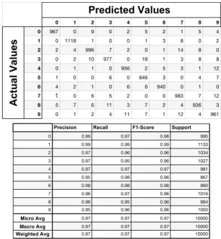
Predicted Values 0 1 2 3 4 5 6 7 8 9 Actual Values 0 967 0 9 0 2 5 2 1 5 4 1 0 1118 1 0 0 1 3 8 0 2 2 2 4 996 7 2 0 1 14 8 0 3 0 2 10 977 0 18 1 3 8 8 4 0 1 1 0 956 2 5 3 1 12 5 1 0 0 6 0 846 3 0 4 7 6 4 2 1 0 6 6 940 0 1 0 7 1 0 6 5 2 0 0 983 7 12 8 5 7 6 11 3 7 2 4 936 3 9 0 1 2 4 11 7 1 12 4 961
Precision Recall F1-Score Support
0 0.99 0.97 0.98 995 1 0.99 0.99 0.99 1133 2 0.97 0.96 0.96 1034 3 0.97 0.95 0.96 1027 4 0.97 0.97 0.97 981 5 0.95 0.98 0.96 867 6 0.98 0.98 0.98 960 7 0.96 0.97 0.96 1016 8 0.96 0.95 0.96 984 9 0.95 0.96 0.96 1003 Micro Avg 0.97 0.97 0.97 10000 Macro Avg 0.97 0.97 0.97 10000 Weighted Avg 0.97 0.97 0.97 10000
Figure 39: Confusion matrix and classification report of the neural network model with sparse autoencoder
ciple for using denoising autoencoders. For achieving this denoising properly, the model requires to extract features that capture useful structure in the distribution of the in-put. Denoising autoencoders apply corrupted data through
stochastic mapping. Our input is x and corrupted data isxe
and stochastic mapping isx ∼ qe D(ex|x).
As its a standard autoencoder, corrupted data ex is
mapped to a hidden layer. h = fθ(ex) = s(Wex + b).
And from this the model reconstructs z = gθ0(h).
Predicted Values 0 1 2 3 4 5 6 7 8 9 Actual Values 0 54 0 29 5 2 13 111 12 20 10 1 0 4 114 4 54 8 7 35 38 17 2 369 416 154 295 77 14 222 252 510 14 3 14 12 315 36 5 338 58 297 80 212 4 2 182 19 2 63 1 161 20 10 188 5 41 1 4 329 11 80 185 1 117 47 6 276 9 11 1 48 89 120 0 57 3 7 22 203 183 72 288 7 0 57 80 411 8 108 308 195 188 73 249 89 83 16 88 9 94 0 8 78 361 93 5 271 46 19
Precision Recall F1-Score Support
0 0.06 0.21 0.09 256 1 0.00 0.01 0.01 281 2 0.15 0.07 0.09 2323 3 0.04 0.03 0.03 1367 4 0.06 0.10 0.08 648 5 0.09 0.10 0.09 816 6 0.13 0.20 0.15 614 7 0.06 0.04 0.05 1323 8 0.02 0.01 0.01 1397 9 0.02 0.02 0.02 975 Micro Avg 0.06 0.06 0.06 10000 Macro Avg 0.06 0.08 0.06 10000 Weighted Avg 0.07 0.06 0.06 10000
Figure 40: Confusion matrix and classification report of the neural network model without sparse autoencoder after FGSM attack Predicted Values 0 1 2 3 4 5 6 7 8 9 Actual Values 0 966 0 7 0 2 4 4 2 3 4 1 0 1121 0 1 1 2 3 8 0 4 2 3 7 996 6 2 0 1 15 9 1 3 1 0 10 976 0 17 2 4 10 6 4 0 1 1 0 952 0 7 3 2 15 5 1 0 0 8 0 849 3 0 5 6 6 6 2 2 0 7 6 934 0 2 0 7 0 1 4 3 2 1 0 977 9 15 8 3 3 9 11 4 8 3 6 930 5 9 0 0 3 5 12 5 1 13 4 953
Precision Recall F1-Score Support
0 0.99 0.97 0.98 992 1 0.99 0.98 0.99 1140 2 0.97 0.96 0.96 1040 3 0.97 0.95 0.96 1026 4 0.97 0.97 0.97 981 5 0.95 0.97 0.96 872 6 0.97 0.97 0.97 959 7 0.95 0.97 0.96 1012 8 0.95 0.95 0.95 982 9 0.94 0.96 0.95 996 Micro Avg 0.97 0.97 0.97 10000 Macro Avg 0.97 0.97 0.97 10000 Weighted Avg 0.97 0.97 0.97 10000
Figure 41: Confusion matrix and classification report of the neural network model with sparse autoencoder after FGSM attack
5.4.1 Multi-Class Logistic Regression of Denoising
Autoencoder
In denoising autoencoder for multi-class logistic regres-sion, the loss does not improve for each epoch. Although it starts better at lower epoch values, in the end, vanilla au-toencoder seems to be better. Sparse auau-toencoder’s loss is slightly worse.
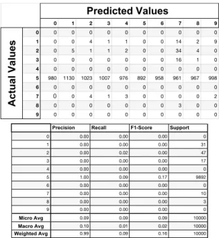
Predicted Values 0 1 2 3 4 5 6 7 8 9 Actual Values 0 0 0 0 0 0 0 0 0 0 0 1 0 0 4 1 1 0 0 14 2 9 2 0 5 1 1 2 0 0 34 4 0 3 0 0 0 0 0 0 0 16 1 0 4 0 0 0 0 0 0 0 0 0 0 5 980 1130 1023 1007 976 892 958 961 967 998 6 0 0 0 0 0 0 0 0 0 0 7 0 0 4 1 3 0 0 0 0 2 8 0 0 0 0 0 0 0 3 0 0 9 0 0 0 0 0 0 0 0 0 0
Precision Recall F1-Score Support
0 0.00 0.00 0.00 0 1 0.00 0.00 0.00 31 2 0.00 0.02 0.00 47 3 0.00 0.00 0.00 17 4 0.00 0.00 0.00 0 5 1.00 0.09 0.17 9892 6 0.00 0.00 0.00 0 7 0.00 0.00 0.00 10 8 0.00 0.00 0.00 3 9 0.00 0.00 0.00 0 Micro Avg 0.09 0.09 0.09 10000 Macro Avg 0.10 0.01 0.02 10000 Weighted Avg 0.99 0.09 0.16 10000
Figure 42: Confusion matrix and classification report of the neural network model without sparse autoencoder after T-FGSM attack Predicted Values 0 1 2 3 4 5 6 7 8 9 Actual Values 0 966 0 9 0 1 3 4 1 4 4 1 0 1121 1 0 1 1 3 9 0 3 2 2 5 998 7 2 0 1 15 7 0 3 0 1 9 974 0 14 1 3 9 7 4 0 1 1 0 954 0 5 3 1 14 5 1 0 0 9 0 862 6 0 5 11 6 5 2 2 0 7 5 935 0 0 0 7 1 0 5 5 2 0 0 981 7 12 8 5 4 6 11 4 3 2 5 938 4 9 0 1 1 4 11 4 1 11 3 954
Precision Recall F1-Score Support
0 0.99 0.97 0.98 992 1 0.99 0.98 0.99 1139 2 0.97 0.96 0.96 1037 3 0.96 0.96 0.96 1018 4 0.97 0.97 0.97 979 5 0.97 0.96 0.97 894 6 0.98 0.98 0.98 956 7 0.95 0.97 0.96 1013 8 0.96 0.96 0.96 982 9 0.95 0.96 0.95 990 Micro Avg 0.97 0.97 0.97 10000 Macro Avg 0.97 0.97 0.97 10000 Weighted Avg 0.97 0.97 0.97 10000
Figure 43: Confusion matrix and classification report of the neural network model with sparse autoencoder after T-FGSM attack
also applies a sharp perturbation, which is presented in Fig-ure 48 and FigFig-ure 49.
We observe that there is a similarity between accuracy results for denoising autoencoder with multi-class logistic regression and sparse autoencoder results. Natural fooling accuracy drops drastically in denoising autoencoder, but non-targeted and one targeted attack seem to be somewhat like sparse autoencoder, one targeted attack having less ac-curacy in denoising autoencoder.
Predicted Values 0 1 2 3 4 5 6 7 8 9 Actual Values 0 4 0 35 4 2 13 122 11 22 10 1 0 4 111 4 33 8 6 32 37 9 2 377 360 10 295 65 5 246 205 494 14 3 14 12 398 11 6 337 68 315 98 211 4 2 150 23 2 15 0 226 20 9 199 5 37 0 2 330 6 23 177 2 110 45 6 299 11 15 1 56 103 11 0 59 5 7 19 223 206 72 278 7 1 18 78 392 8 118 374 218 190 89 272 94 95 16 102 9 110 1 14 101 432 124 7 330 51 22
Precision Recall F1-Score Support
0 0.00 0.02 0.01 223 1 0.00 0.02 0.01 244 2 0.01 0.00 0.01 2071 3 0.01 0.01 0.01 1470 4 0.02 0.02 0.02 646 5 0.03 0.03 0.03 732 6 0.01 0.02 0.01 560 7 0.02 0.01 0.02 1294 8 0.02 0.01 0.01 1568 9 0.02 0.02 0.02 1192 Micro Avg 0.01 0.01 0.01 10000 Macro Avg 0.01 0.02 0.01 10000 Weighted Avg 0.01 0.01 0.01 10000
Figure 44: Confusion matrix and classification report of the neural network model without sparse autoencoder after basic iterative method attack
Predicted Values 0 1 2 3 4 5 6 7 8 9 Actual Values 0 964 0 6 0 2 4 4 2 3 4 1 0 1119 0 1 1 1 3 8 0 3 2 3 8 998 6 2 0 1 14 8 1 3 1 0 10 972 0 21 2 5 12 7 4 0 1 1 0 955 1 11 2 2 19 5 1 0 0 8 0 844 4 0 5 7 6 7 2 2 0 7 7 929 0 2 0 7 0 1 4 5 2 1 0 974 7 19 8 4 4 9 13 4 9 3 7 931 5 9 0 0 2 5 9 4 1 16 4 944
Precision Recall F1-Score Support
0 0.98 0.97 0.98 989 1 0.99 0.99 0.99 1136 2 0.97 0.96 0.96 1041 3 0.96 0.94 0.95 1030 4 0.97 0.96 0.97 992 5 0.95 0.97 0.96 869 6 0.97 0.97 0.97 956 7 0.95 0.96 0.95 1013 8 0.96 0.94 0.95 989 9 0.94 0.96 0.95 985 Micro Avg 0.96 0.96 0.96 10000 Macro Avg 0.96 0.96 0.96 10000 Weighted Avg 0.96 0.96 0.96 10000
Figure 45: Confusion matrix and classification report of the neural network model with sparse autoencoder after basic iterative method attack
5.4.2 Neural Network of Denoising Autoencoder
We investigate that neural network accuracy for denoising autoencoder is worse than sparse autoencoder results and vanilla autoencoder results. It is still a useful autoencoder for denoising corrupted data and other purposes; however, it is not the right choice just for robustness against adver-sarial examples.
Figure 46: Optimized Relu Loss History for Denoising Au-toencoder
Figure 47: Comparison of accuracy with and without de-noising autoencoder for non-targeted attack
Figure 48: Value change and perturbation of a non-targeted attack on model without denoising autoencoder
Figure 49: Value change and perturbation of a non-targeted attack on model with denoising autoencoder
5.5
Variational Autoencoder
In this study, we examine variational autoencoders as the fi-nal type of autoencoder type. The variatiofi-nal autoencoders have an encoder and a decoder, although their mathemat-ical formulation differs significantly. They are associated with Generative Adversarial Networks due to their archi-tectural similarity. In summary, variational autoencoders are also generative models. Differently, from sparse au-toencoders, denoising auau-toencoders, and vanilla autoen-coders, all of which aim discriminative modeling, gener-ative modeling tries to simulate how the data can be gen-erated and to understand the underlying causal relations. It also considers these causal relations when generating new
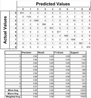
Figure 50: Comparison of accuracy with and without de-noising autoencoder for targeted attacks. AE stands for the models with denoising autoencoder, WO stands for models without autoencoder Predicted Values 0 1 2 3 4 5 6 7 8 9 Actual Values 0 974 0 3 0 0 2 7 1 5 3 1 0 1125 5 0 0 0 3 2 0 3 2 1 4 1009 4 1 0 2 10 3 0 3 0 2 0 999 0 5 0 3 1 2 4 0 0 2 0 973 0 3 0 1 10 5 0 0 0 3 0 877 1 0 1 4 6 1 1 0 0 3 4 938 0 0 0 7 1 1 10 2 0 2 0 1006 4 5 8 3 2 3 2 1 2 4 2 957 3 9 0 0 0 0 4 0 0 4 2 979
Precision Recall F1-Score Support
0 0.99 0.98 0.99 995 1 0.99 0.99 0.99 1138 2 0.98 0.98 0.98 1034 3 0.99 0.99 0.99 1012 4 0.99 0.98 0.99 989 5 0.98 0.99 0.99 886 6 0.98 0.99 0.98 947 7 0.98 0.98 0.98 1031 8 0.98 0.98 0.98 979 9 0.97 0.99 0.98 989 Micro Avg 0.98 0.98 0.98 10000 Macro Avg 0.98 0.98 0.98 10000 Weighted Avg 0.98 0.98 0.98 10000
Figure 51: Confusion matrix and classification report of the neural network model without denoising autoencoder
data.
Variational autoencoders use an estimator algorithm called Stochastic Gradient Variational Bayes for training.
This algorithm assumes the data is generated by pθ(x|h)
which is a directed graphical model and θ being the pa-rameters of decoder, in variational autoencoder’s case, the parameters of the generative model. The encoder is
learn-ing an approximation of qφ(h|x) to a posterior distribution
which is showed by pθ(x|h) and φ being the parameters of
the encoder; in variational autoencoder’s case, the param-eters of recognition model. We will use Kullback-Leibler
divergence again, showed as DKL.
L = (φ, θ, x) = DKL(qφ(h|x)||pθ(h)) −
Eqφ(h|x)(logpθ(x|h)).
Variational and likelihood distributions’ shape is chosen by factorized Gaussians. The encoder outputs are p(x) and
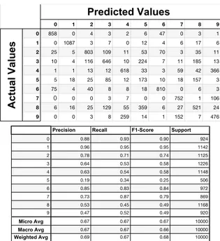
like-Predicted Values 0 1 2 3 4 5 6 7 8 9 Actual Values 0 961 0 2 0 1 2 7 1 7 3 1 1 1119 7 0 2 0 2 8 2 3 2 5 3 992 7 3 0 1 10 6 0 3 1 1 10 980 1 16 1 8 20 10 4 1 0 1 0 937 3 1 0 5 12 5 3 1 0 7 0 852 5 0 5 4 6 6 5 1 1 6 7 937 0 3 0 7 1 0 11 7 4 0 0 984 3 11 8 1 5 8 5 2 7 3 4 913 7 9 0 1 0 3 26 5 1 13 10 959
Precision Recall F1-Score Support
0 0.98 0.98 0.98 984 1 0.99 0.98 0.98 1144 2 0.96 0.97 0.96 1027 3 0.97 0.94 0.95 1048 4 0.95 0.98 0.96 960 5 0.96 0.97 0.96 877 6 0.98 0.97 0.97 966 7 0.96 0.96 0.96 1021 8 0.94 0.96 0.95 955 9 0.95 0.94 0.95 1018 Micro Avg 0.96 0.96 0.96 10000 Macro Avg 0.96 0.96 0.96 10000 Weighted Avg 0.96 0.96 0.96 10000
Figure 52: Confusion matrix and classification report of the neural network model with denoising autoencoder
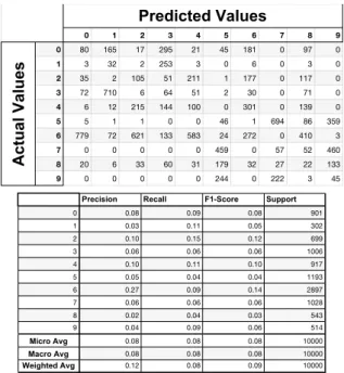
Predicted Values 0 1 2 3 4 5 6 7 8 9 Actual Values 0 82 0 22 7 15 5 71 4 18 7 1 0 8 121 5 85 2 6 42 39 18 2 200 365 86 255 54 15 141 210 304 8 3 9 12 352 54 6 302 47 329 155 114 4 9 272 36 2 69 0 282 50 14 280 5 83 7 8 345 19 92 212 6 232 78 6 303 20 8 1 25 56 77 0 53 1 7 11 206 181 68 278 2 1 56 57 350 8 146 244 213 218 84 352 120 77 16 141 9 137 1 5 55 347 66 1 254 86 12
Precision Recall F1-Score Support
0 0.08 0.35 0.14 231 1 0.01 0.02 0.01 326 2 0.08 0.05 0.06 1638 3 0.05 0.04 0.05 1380 4 0.07 0.07 0.07 1014 5 0.10 0.09 0.09 1082 6 0.08 0.14 0.10 544 7 0.05 0.05 0.05 1210 8 0.02 0.01 0.01 1611 9 0.01 0.01 0.01 964 Micro Avg 0.06 0.06 0.06 10000 Macro Avg 0.06 0.08 0.06 10000 Weighted Avg 0.06 0.06 0.05 10000
Figure 53: Confusion matrix and classification report of the neural network model without denoising autoencoder after FGSM attack
lihood term of variational objective is defined below.
qφ(h|x) = N (p(x), w2(x)I)
pθ(x|h) = N (µ(h), σ2(h)I)
5.5.1 Multi-Class Logistic Regression of Variational
Autoencoder
The findings from Figure 59 show that variational autoen-coder indicates the best loss function result. However, Fig-ure 60 presents that the accuracy is low, especially in low
Predicted Values 0 1 2 3 4 5 6 7 8 9 Actual Values 0 961 0 1 0 2 2 7 1 6 3 1 1 1120 7 1 3 0 2 7 2 4 2 5 3 993 7 2 0 1 10 7 0 3 1 1 11 977 2 16 1 10 18 9 4 1 0 1 0 935 3 1 1 6 11 5 3 1 0 7 0 855 4 0 6 3 6 5 4 2 1 7 5 938 0 3 0 7 1 0 9 8 4 0 0 981 3 11 8 1 6 8 6 3 7 3 4 914 7 9 1 0 0 3 24 4 1 14 9 961
Precision Recall F1-Score Support
0 0.98 0.98 0.98 983 1 0.99 0.98 0.98 1147 2 0.96 0.97 0.96 1028 3 0.97 0.93 0.95 1046 4 0.95 0.97 0.96 959 5 0.96 0.97 0.97 879 6 0.98 0.97 0.98 965 7 0.95 0.96 0.96 1017 8 0.94 0.95 0.95 959 9 0.95 0.94 0.95 1017 Micro Avg 0.96 0.96 0.96 10000 Macro Avg 0.96 0.96 0.96 10000 Weighted Avg 0.96 0.96 0.96 10000
Figure 54: Confusion matrix and classification report of the neural network model with denoising autoencoder after FGSM attack Predicted Values 0 1 2 3 4 5 6 7 8 9 Actual Values 0 0 0 0 0 0 0 0 0 0 0 1 0 0 0 0 3 0 0 0 1 0 2 0 10 0 0 1 0 0 0 2 0 3 0 0 0 0 0 0 1 1 0 0 4 0 0 0 0 0 0 0 0 0 0 5 980 1125 1032 1010 976 892 957 1026 971 1009 6 0 0 0 0 2 0 0 0 0 0 7 0 0 0 0 0 0 0 0 0 0 8 0 0 0 0 0 0 0 1 0 0 9 0 0 0 0 0 0 0 0 0 0
Precision Recall F1-Score Support
0 0.00 0.00 0.00 0 1 0.00 0.00 0.00 4 2 0.00 0.00 0.00 13 3 0.00 0.00 0.00 2 4 0.00 0.00 0.00 0 5 1.00 0.09 0.16 9978 6 0.00 0.00 0.00 2 7 0.00 0.00 0.00 0 8 0.00 0.00 0.00 1 9 0.00 0.00 0.00 0 Micro Avg 0.09 0.09 0.09 10000 Macro Avg 0.10 0.01 0.02 10000 Weighted Avg 1.00 0.09 0.16 10000
Figure 55: Confusion matrix and classification report of the neural network model without denoising autoencoder after T-FGSM attack
epsilon values where even autoencoded data gives worse accuracy than the normal learning process.
Perturbation applied by variational autoencoder is not as sharp in sparse autoencoder and denoising autoencoder. It seems similar to vanilla autoencoder’s perturbation.
The variational autoencoder has the worst results. Be-sides, it presents bad results at the low values of epsilon, making autoencoded data less accurate and only a slight improvement compared to the normal data in high values of epsilon.
Predicted Values 0 1 2 3 4 5 6 7 8 9 Actual Values 0 0 0 0 0 0 0 0 0 0 0 1 0 0 0 0 0 0 0 0 0 0 2 340 374 1018 773 30 88 6 14 571 28 3 0 0 0 0 0 0 0 0 0 0 4 0 0 0 0 0 0 0 0 0 0 5 0 0 0 0 0 0 0 0 0 0 6 621 274 2 20 269 579 949 0 218 27 7 19 487 12 217 683 225 3 1014 185 954 8 0 0 0 0 0 0 0 0 0 0 9 0 0 0 0 0 0 0 0 0 0
Precision Recall F1-Score Support
0 0.00 0.00 0.00 0 1 0.00 0.00 0.00 0 2 0.99 0.31 0.48 3242 3 0.00 0.00 0.00 0 4 0.00 0.00 0.00 0 5 0.00 0.00 0.00 0 6 0.99 0.32 0.48 2959 7 0.99 0.27 0.42 3799 8 0.00 0.00 0.00 0 9 0.00 0.00 0.00 0 Micro Avg 0.30 0.30 0.30 10000 Macro Avg 0.30 0.09 0.14 10000 Weighted Avg 0.99 0.30 0.46 10000
Figure 56: Confusion matrix and classification report of the neural network model with denoising autoencoder after T-FGSM attack Predicted Values 0 1 2 3 4 5 6 7 8 9 Actual Values 0 2 0 23 6 18 5 67 4 18 7 1 0 7 116 3 57 2 7 38 37 12 2 207 323 20 263 34 5 165 190 291 5 3 5 4 384 8 5 310 37 337 163 108 4 10 273 40 1 7 0 304 49 15 285 5 56 1 5 336 14 14 216 5 216 67 6 331 15 8 1 31 64 12 0 58 1 7 12 202 190 76 289 2 0 18 59 346 8 184 308 239 238 120 415 149 84 14 161 9 173 2 7 78 407 75 1 303 103 17
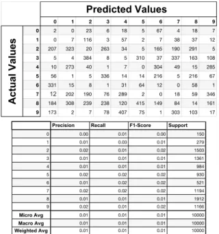
Precision Recall F1-Score Support
0 0.00 0.01 0.00 150 1 0.01 0.03 0.01 279 2 0.02 0.01 0.02 1503 3 0.01 0.01 0.01 1361 4 0.01 0.01 0.01 984 5 0.02 0.02 0.02 930 6 0.01 0.02 0.02 521 7 0.02 0.02 0.02 1194 8 0.01 0.01 0.01 1912 9 0.02 0.01 0.02 1166 Micro Avg 0.01 0.01 0.01 10000 Macro Avg 0.01 0.01 0.01 10000 Weighted Avg 0.01 0.01 0.01 10000
Figure 57: Confusion matrix and classification report of the neural network model without denoising autoencoder after basic iterative method attack
5.5.2 Neural Network of Variational Autoencoder
Variational autoencoder with neural networks also illus-trates the worst results compared to other autoencoder types, where the accuracy for autoencoded data against an attack has around between 0.96 and 0.99 accuracies, vari-ational autoencoder has around between 0.65 and 0.70 ac-curacies. Predicted Values 0 1 2 3 4 5 6 7 8 9 Actual Values 0 0 0 0 0 0 0 0 0 0 0 1 0 0 0 0 0 0 0 0 0 0 2 351 391 1017 773 30 89 6 16 577 28 3 0 0 0 0 0 0 0 0 0 0 4 0 0 0 0 0 0 0 0 0 0 5 0 0 0 0 0 0 0 0 0 0 6 609 273 3 17 261 575 949 0 212 26 7 20 471 12 220 691 228 3 1012 185 955 8 0 0 0 0 0 0 0 0 0 0 9 0 0 0 0 0 0 0 0 0 0
Precision Recall F1-Score Support
0 0.00 0.00 0.00 0 1 0.00 0.00 0.00 0 2 0.99 0.31 0.47 3278 3 0.00 0.00 0.00 0 4 0.00 0.00 0.00 0 5 0.00 0.00 0.00 0 6 0.99 0.32 0.49 2925 7 0.98 0.27 0.42 3797 8 0.00 0.00 0.00 0 9 0.00 0.00 0.00 0 Micro Avg 0.30 0.30 0.30 10000 Macro Avg 0.30 0.09 0.14 10000 Weighted Avg 0.99 0.30 0.46 10000
Figure 58: Confusion matrix and classification report of the neural network model with denoising autoencoder after basic iterative method attack
Figure 59: Optimized Relu Loss History for Variational Autoencoder
Figure 60: Comparison of accuracy with and without vari-ational autoencoder for non-targeted attack
6
Experiments with Fashion MNIST
Dataset
6.1
Introduction
We also used Fashion MNIST dataset. We will briefly show the experiment results for not filling the paper with