a thesis
submitted to the department of computer engineering
and the institute of engineering and science
of bilkent university
in partial fulfillment of the requirements
for the degree of
master of science
By
Do˘
gan Altunbay
July, 2010
Assist. Prof. Dr. C¸ i˘gdem G¨und¨uz Demir(Advisor)
I certify that I have read this thesis and that in my opinion it is fully adequate, in scope and in quality, as a thesis for the degree of Master of Science.
Assist. Prof. Dr. Selim Aksoy
I certify that I have read this thesis and that in my opinion it is fully adequate, in scope and in quality, as a thesis for the degree of Master of Science.
Assist. Prof. Dr. Tolga Can
Approved for the Institute of Engineering and Science:
Prof. Dr. Levent Onural Director of the Institute
STRUCTURAL ANALYSIS OF TISSUE IMAGES
Do˘gan Altunbay
M.S. in Computer Engineering
Supervisor: Assist. Prof. Dr. C¸ i˘gdem G¨und¨uz Demir July, 2010
Computer aided image analysis tools are becoming increasingly important in automated cancer diagnosis and grading. They have the potential of assisting pathologists in histopathological examination of tissues, which may lead to a considerable amount of subjectivity. These analysis tools help reduce the sub-jectivity, providing quantitative information about tissues. In literature, it has been proposed to implement such computational tools using different methods that represent a tissue with different set of image features. One of the most com-monly used methods is the structural method that represents a tissue quantifying the spatial relationship of its components. Although previous structural methods lead to promising results for different tissue types, they only use the spatial rela-tions of nuclear tissue components without considering the existence of different components in a tissue. However, additional information that could be obtained from other components of the tissue has an importance in better representing the tissue, and thus, in making more reliable decisions.
This thesis introduces a novel structural method to quantify histopathological images for automated cancer diagnosis and grading. Unlike the previous struc-tural methods, it proposes to represent a tissue considering the spatial distribution of different tissue components. To this end, it constructs a graph on multiple tis-sue components and colors its edges depending on the component types of their end points. Subsequently, a new set of structural features is extracted from these “color graphs” and used in the classification of tissues. Experiments conducted on 3236 photomicrographs of colon tissues that are taken from 258 different pa-tients demonstrate that the color graph approach leads to 94.89 percent training accuracy and 88.63 percent test accuracy. Our experiments also show that the introduction of color edges to represent the spatial relationship of different tissue
components and the use of graph features defined on these color edges signifi-cantly improve the classification accuracy of the previous structural methods.
Keywords: medical image analysis, graph theory, histopathological image
RENKL˙I C
¸ ˙IZGE G ¨
OSTER˙IM˙I
Do˘gan Altunbay
Bilgisayar M¨uhendisli˘gi, Y¨uksek Lisans
Tez Y¨oneticisi: Yar. Do¸c. Dr. C¸ i˘gdem G¨und¨uz Demir Temmuz, 2010
Bilgisayar destekli g¨or¨unt¨u analizi ara¸cları, otomatikle¸stirilmi¸s kanser tanı ve derecelendirmesi alanında giderek ¨onemli hale gelmektedir. Bu ara¸cların, kayda de˘ger ¨oznelliklere neden olabilen doku histopatolojik incelemesinde patologlara yardımcı olma potansiyelleri bulunmaktadır. Bu analiz ara¸cları, dokular ile ilgili nicel bilgi sa˘glayarak ¨oznelli˘gin azaltılmasına yardımcı olmaktadır. Literat¨urde, bu tip hesaplamasal ara¸cların, dokuyu farklı imge ¨oznitelikleri ile g¨osteren farklı y¨ontemler kullanarak geli¸stirilmesi ¨onerilmi¸stir. En ¸cok kullanılan y¨ontemlerden biri, doku bile¸senleri arasındaki uzamsal ili¸skiyi niceleyerek dokuyu temsil eden yapısal y¨ontemdir. ¨Onceki yapısal y¨ontemler ile de˘gi¸sik doku t¨urleri i¸cin umut verici sonu¸clar elde edilmesine ra˘gmen, bu y¨ontemler, bir dokunun nicelenmesi i¸cin yalnızca ¸cekirdek bile¸senlerini kullanmakta ve dokudaki di˘ger bile¸senlerin varlı˘gını dikkate almamaktadır. ¨Ote yandan, bir dokunun de˘gi¸sik bile¸senlerinden elde edilebilecek ek bilgi, bu dokunun daha iyi g¨osterilmesinde, ve dolayısıyla daha g¨uvenilir kararlar alınmasında ¨onemlidir.
Bu tez, otomatik kanser tanı ve derecelendirmesi i¸cin histopatolojik
imgelerin nicelenmesinde kullanılabilecek yeni bir yapısal y¨ontem sunmaktadır. ¨
Onceki y¨ontemlerin aksine, ¨onerilen y¨ontem, farklı doku bile¸senlerinin uzamsal da˘gılımlarını dikkate alarak dokuyu temsil etmeyi ¨onermektedir. Bu ama¸cla, ¨
onerilen y¨ontem farklı doku bile¸senlerin ¨uzerinde bir ¸cizge tanımlar ve bu ¸cizgenin kenarlarını u¸c bile¸senlerinin t¨urlerine g¨ore renklendirir. Ardından, elde edilen bu “renkli ¸cizgeler”den yeni bir yapısal ¨oznitelik k¨umesi ¸cıkarır ve bu k¨umeyi dokuların sınıflandırılmasında kullanır. 258 farklı hastadan alınan 3236 kolon doku imgesi ¨uzerinde yapılan deneyler, ¨onerilen renkli ¸cizge y¨onteminin, ¨
o˘grenme seti i¸cin y¨uzde 94.89 ve test seti i¸cin y¨uzde 88.63 do˘gruluk verdi˘gini g¨ostermektedir. Deneylerimiz ayrıca, farklı doku bile¸senleri arasındaki uzamsal ili¸skiyi g¨osteren renkli kenarların tanımlanmasının ve bunlar ¨uzerinde ¸cıkarılan
¸cizge ¨ozniteliklerinin kullanımının, ¨onceki yapısal y¨ontemlerin sınıflandırma ba¸sarısını kayda de˘ger ¨ol¸c¨ude artırdı˘gını g¨ostermektedir.
Anahtar s¨ozc¨ukler : Medikal g¨or¨unt¨u analizi, ¸cizge teorisi, histopatolojik g¨or¨unt¨u analizi, kanser tanı ve derecelendirilmesi.
I present my thanks and respect to my advisor Assist. Prof. Dr. C¸ i˘gdem G¨und¨uz Demir for her motivating guidance throughout this study. I also thank Assist.
Prof. Dr. Selim Aksoy and Assist. Prof. Dr. Tolga Can for accepting to
participate in my thesis committee.
I am grateful to my parents, G¨ul¸sen and Hakim Altunbay, my brothers, Cihan and Hakan Can Altunbay, and my fiance, B¨u¸sra A¸slar, for their endless support.
Do˘gan Altunbay July 2010
1 Introduction 1 1.1 Motivation . . . 2 1.2 Contribution . . . 4 1.3 Outline of Thesis . . . 6 2 Background 7 2.1 Domain Description . . . 7
2.2 Computer Aided Diagnosis and Grading of Cancer . . . 11
2.2.1 Morphological Methods . . . 12
2.2.2 Textural Methods . . . 12
2.2.3 Structural Methods . . . 18
3 Methodology 26 3.1 Node Identification . . . 28
3.1.1 Clustering with K-means . . . 28
3.1.2 Circle Fitting . . . 31 viii
3.2 Edge Identification . . . 33
3.3 Feature Extraction . . . 34
3.3.1 Average Degree . . . 36
3.3.2 Average Clustering Coefficient . . . 36
3.3.3 Diameter . . . 37
3.4 Classification . . . 38
3.4.1 Support Vector Machines . . . 38
3.4.2 Feature Selection . . . 40
4 Experiments and Results 42 4.1 Dataset . . . 42
4.2 Classification Results . . . 43
4.2.1 Results for Color Graph Features . . . 44
4.2.2 Results for Forward Selection . . . 46
4.2.3 Results for Backward Elimination . . . 48
4.3 Analysis of the Method . . . 51
4.3.1 Analysis of Node Identification . . . 53
4.3.2 Analysis of Parameters . . . 56
4.4 Comparisons . . . 59
4.4.1 Colorless Graphs . . . 59
4.4.3 Statistical Tests . . . 62
1.1 Histological image of a typical colon tissue and the corresponding color graph representation. . . 5
2.1 Microscopic view of a colon tissue section. . . 9
2.2 Histopathological images of colon tissues. . . 10
2.3 Delaunay triangulation of 20 random points in 2 dimensional
Eu-clidean space. . . 20
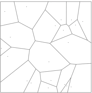
2.4 Voronoi diagram of the point set used in Figure 2.3. . . 21
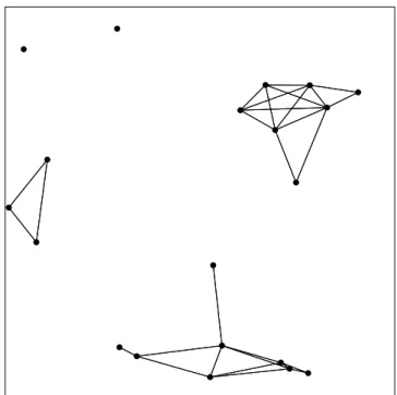
2.5 Gabriel’s graph of the point set used in Figure 2.3. . . 22
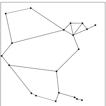
2.6 Minimum spanning tree of the Delaunay triangulation given in
Figure 2.3. . . 23 2.7 Probabilistic graph generated on the point set given in Figure 2.3.
Here, Equation 2.3 is used with α = 2 and r = 0.2. . . . 24
3.1 Overview of the color graph approach. . . 27
3.2 Pixel clusters of histopathological images given in Figure 2.2 that are obtained using k-means. . . 30
3.3 Circular primitives that are obtained by applying the circle fitting algorithm to pixel clusters of images given in Figure 3.2. . . 32
3.4 Color graphs that are generated from the graph nodes given in
Figure 3.3 and that are colored with one of the six colors given in
Table 3.1 depending on the component types of their end nodes. . 35
3.5 (a) Three possible separating lines, and (b) the separating line with maximum margin. . . 39
3.6 (a) Data points in two dimensional space that are non-linearly
separable, and (b) the data points obtained by transforming these points using kernel method. . . 40
4.1 Sample images of (a) - (b) normal, (c) - (d) low-grade cancerous,
and (e) - (f) high-grade cancerous tissues that are misclassified by color graph approach. . . 45 4.2 Classification accuracies of (a) the training set and (b) the test set
with respect to iterations of forward selection. . . 47 4.3 Classification accuracies of (a) training and (b) test sets with
re-spect to iterations of backward elimination. . . 50 4.4 Classification accuracies of (a) the training set and (b) the test set
as a function of modification percentage. . . 54 4.5 Classification accuracies of (a) the training set and (b) the test set
as a function of the structuring element size. . . 57 4.6 Classification accuracies of (a) the training set and (b) the test set
as a function of the area threshold, which is used in circle fitting. 58
4.7 Colorless graphs of histopathological images given in Figure 2.2. . 60
4.8 Delaunay triangulations of histopathological images given in
2.1 Haralick features obtained from gray level co-occurrence matrices. 14 2.2 Gray level run length features. . . 16
2.3 Structural features obtained from different graph based
represen-tations: Voronoi diagrams (VD), Delaunay triangulations (DT), Gabriel’s graphs (GG), minimum spanning tree (MST), and probabilistic graphs (PG). . . . 19
3.1 List of colors that are used for labeling triangle edges. . . 34
4.1 Confusion matrices obtained with the color graph approach for
(a) the training set and (b) the test set, and (c) average accuracy results and their standard deviations obtained by applying leave-one-patient-out cross validation on the test set. These results are obtained when all color graph features are used. . . 44 4.2 List of features selected by forward selection. . . 48
4.3 Confusion matrices obtained with the color graph approach for
(a) the training set and (b) the test set, and (c)average accuracy results and their standard deviations obtained by applying leave-one-patient-out cross validation of the test set. These results are obtained using a subset of color graph features determined by for-ward selection. . . 49
4.4 List of features selected by backward elimination. . . 51
4.5 Confusion matrices obtained with the color graph approach for
(a) the training set and (b) the test set, and (c) average accu-racy results and their standard deviations obtained by applying leave-one-patient-out cross validation of the test set. These results are obtained using a subset of color graph features determined by backward elimination. . . 52
4.6 Confusion matrices obtained with the colorless graph features for
(a) the training set and (b) the test set, and (c) average accuracy results and their standard deviations obtained by applying leave-one-patient-out cross validation of the test set. . . 61
4.7 Confusion matrices obtained with the Delaunay triangulation
fea-tures for (a) the training set and (b) the test set, and (c) average accuracy results and their standard deviations obtained by apply-ing leave-one-patient-out cross validation of the test set. . . 64 4.8 2× 2 contingency matrix of McNemar’s test . . . 65 4.9 3× 3 contingency tables for (a) color graphs vs. colorless graphs,
and (b) color graphs vs. Delaunay triangulations. . . 66
4.10 Computed χ2 values and their corresponding P values for colorless
Introduction
Cancer is a member of neoplastic diseases. It may occur in various tissue types and in different forms, and causes abnormal growth and change in the cellular structure of tissues from which it originates. With the increased malignancy level of cancer, tissues eventually lose their distinguishing characteristics. This situa-tion may result in the interrupsitua-tion of the vital funcsitua-tions of organs, which makes cancer one of the most lethal diseases [1, 46, 63]. However, with its early detec-tion and the correct treatment selecdetec-tion, for which cancer grade is an important factor, survival rates greatly increase. A considerable amount of effort has been put in the field of cancer diagnosis and grading. Medical experts take advantage of numerous medical imaging techniques such as Magnetic Resonance Imaging (MRI), Computer Aided Tomography (CAT), Mammography, Colonoscopy, Ul-trasound Imaging for cancer screening. Although these methods provide effective diagnosis tools for screening and early detection of tumors, they may not be help-ful in determining their malignancy level. Moreover, these methods are not used as the gold standard and biopsy examination is still necessary to reach the final decision.
In the current practice of medicine, histopathological examination is the rou-tinely used method to examine biopsies for cancer diagnosis and grading [40, 68]. In this examination, a biopsy specimen is surgically removed from the patient and prepared following suitable fixation and staining procedures. Afterwards,
a pathologist visually inspects the biopsy under a microscope and determines how much the tissue differentiates from its normal appearance. The pathologist then makes a decision about the existence of cancer, and its grade depending on his/her observation.
The extent of differentiation in the tissue, which is determined by histopatho-logical examination, serves as a basis in the choice of relevant medical and/or sur-gical treatment method. Early detection and correct grading of cancer affect the success of the selected treatment method and increase the chance of survival [2]. Therefore, it is important to use procedures that provide efficient information about the malignancy of tissues. Although histopathological examination pro-vides efficient information for accurate diagnosis and grading [59, 64, 14, 20], it is subject to a considerable amount of subjectivity as it is mainly based on visual interpretation of pathologists, which also requires expertise in the field. Based on their experience and interpretation, different pathologists may come up with different decisions for the same tissue. Moreover, a pathologist may make differ-ent decisions for the same tissue at differdiffer-ent times. This inter and intra observer variability may reach significant levels [93, 33] and directly affects the accuracy of the procedure.
Such observer variability reveals a necessity for employing quantitative in-formation to assist the pathologists during the diagnosis and grading processes. Many studies have proposed computational methods in order to obtain quanti-tative information about tissues. These methods are used for developing com-puterized diagnosis tools that provide estimates of the malignancy level and help alleviate the subjectivity of the pathologists.
1.1
Motivation
There are numerous studies that focus on the computer aided diagnosis and grad-ing of cancer. These studies propose image analysis frameworks that employ com-putational methods for the quantification of tissues. These frameworks make use
of morphological, textural, and structural properties of histopathological images to represent a tissue for its quantification.
The morphological approach relies on the use of shape and size characteristics of cellular components. For this purpose, it extracts features such as area, perime-ter, roundness, and symmetry for the quantification of a tissue [106, 86, 88]. The computation of these features transforms pixel level information to component level information. On the other hand, this computation requires segmenting the tissue in order to identify exact boundaries of its components. Complex structure of a typical histopathological image increases the difficulty in segmentation, and may necessitate the manual segmentation of the tissue.
In the textural approach, a tissue is represented with texture characteristics of either the whole tissue [37, 38, 82] or particular components of the tissue such as nuclei [19, 103, 101, 48]. The studies make use of textural features that are computed from co-occurrence matrices [37, 82, 38], run length matrices [104, 4], multiwavelet coefficients [101, 27, 62], and fractal geometry [8, 34, 39]. The defi-nition of these features primarily depends on the pixels of tissue images, thus they are sensitive to noise in the pixel values. Besides, there could be a large amount of noise in a typical histopathological image due to the problems occurred in staining and sectioning [48]. Statistical features computed from histograms of pixel intensities such as average, standard deviation, and entropy [105], and opti-cal densities of nuclear tissue components are also used [104] for quantifying the texture characteristics of a tissue. However, histopathological images of differ-ent tissue types usually have similar intensity distributions as they are stained using the same procedure, and this introduces an important drawback for these methods.
The structural approach provides a higher level representation of a tissue using the spatial relationships and neighborhood properties of their cellular com-ponents. To this end, a graph is constructed on the cellular components and a set of local and global graph features is extracted [37, 104]. In literature, there are different methods of generating graphs. The most common method is to use De-launay triangulations (and their corresponding Voronoi diagrams) where nuclear
components of the tissue are considered as graph nodes [102, 65, 90, 52, 36, 17]. Minimum spanning trees obtained from these graph based representations are also used for representation. Another method is to use probabilistic graphs in which nuclear components are considered as graph nodes, and edges are probabilistically assigned between these nodes [53, 30, 29, 11].
1.2
Contribution
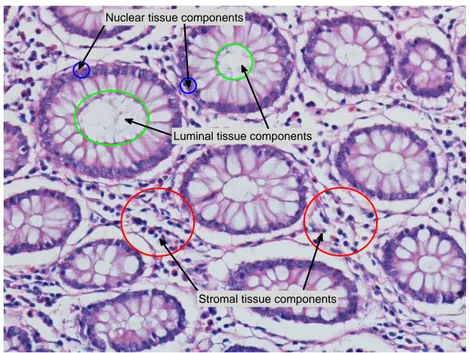
The aforementioned structural methods provide powerful frameworks for comput-erized cancer diagnosis and grading. On the other hand, these methods consider nuclear components of tissues, ignoring the existence of other tissue components such as luminal and stromal regions. Nevertheless, information extracted also considering these additional tissue components may improve the effectiveness of the representation. This improvement can be significant especially for tissues where the components are hierarchically organized. Colon tissues are the exam-ples of such tissues. They are formed of nuclear, luminal, and stromal tissue components. Nuclei of the epithelial cells of colon tissue are lined up around its luminal components and form glandular structures of the colon. Stromal tissue components are distributed between these glandular regions. This hierarchical organization of its nuclear, luminal, and stromal components reflects the major characteristics of the colon tissue. Figure 1.1a shows the histopathological tissue image of a colon tissue section. As observed in this figure, in addition to nuclear components, the distribution of luminal and stromal tissue components has an important role in describing the colon tissue structure. Pathologists also take advantage of spatial distributions of these tissue components in histopathological examination. Therefore, considering additional information obtained from these components in a structural representation will result in a better tissue quantifi-cation.
This thesis introduces a novel structural representation in which the spatial re-lationships of nuclear, stromal, and luminal tissue components are considered [5]. This new representation is used for automated diagnosis and grading of cancer.
Nuclear tissue components
Luminal tissue components
Stromal tissue components
(a) A typical colon tissue
(b) Color graph representation of the tissue image shown in (a)
Figure 1.1: Histological image of a typical colon tissue and the corresponding color graph representation.
The proposed representation first segments a tissue image into its components, transforming image pixels into circular primitives with the use of a heuristic ap-proach described in [94, 55]. Considering these components as nodes, a graph is constructed using Delaunay triangulation. Afterwards, each edge of the triangu-lation is assigned a color label based on the types of its end nodes. Figure 1.1b shows the corresponding color graph representation of the tissue image given in Figure 1.1a. A set of new features is introduced for the constructed “color graph”, which quantifies the relationship of different types of graph nodes (tissue components), and used for classification.
Experiments conducted on 3236 images taken from 258 patients have shown that color graph method yields accurate results for a three class classification problem on colon cancer, and outperforms previous structural methods. We have also shown that introduction of new features that quantify spatial relationships and neighborhood characteristics of different tissue components improves the dis-criminative power of graph based representation.
1.3
Outline of Thesis
The outline of this thesis is as follows. Chapter 2 provides background information about the problem domain, and summarizes previous computational methods on automated cancer diagnosis and grading. Chapter 3 provides detailed descriptions of the proposed color graph representation and newly introduced graph features. Chapter 4 gives the experimental setup and reports the results of automated colon cancer diagnosis and grading. Additionally, Chapter 4 gives the evaluation of the color graph method and its comparisons with other structural methods. Chapter 5 includes concluding remarks and discussions.
Background
This chapter provides background information about the studies in the field of computer aided cancer diagnosis and grading. In the first section, the structure of a colon tissue is described and the information of colon cancer, which is the
cancer type of interest in this thesis, is given. In the second section, image
analysis methods that are employed by the previous studies on computer aided cancer diagnosis and grading are explained.
2.1
Domain Description
Gastrointestinal system of the human body is responsible for processing food
for energy and excreting the solid waste out of the body. Colon is the first
and the longest part of the large intestine and is formed of epithelial cells. The distinctive characteristics of colon epithelium is that it contains a large number of glandular structures. Glands in the colon tissue are responsible for two operations; absorbing water and mineral nutrients from the feces back into the blood and secreting mucus into the colon lumen for lubricating the dehydrated feces.
Colon cancer is a tumor forming type of cancer and it develops in the colon epithelium. It is the third most common cancer incidence among both men and
women in Northern America [1]. Development of colon cancer is usually spread out over a time period of years. It usually begins as a noncancerous polyp, a growth of epithelial tissue that occurs on the lining of the colon, which may later change into cancer. Adenomatous polyps or adenomas are the kind of polyps which have glandular origin and are most likely to become cancerous.
According to the studies, more than half of all individuals will eventually develop one or more adenomas [81]. Although most adenomas are benign which do not turn into cancer, a considerable amount of them are malignant and turn into adenocarcinomas which account for 96 percent of colon cancers [87]. When it turns into cancer, an adenocarcinoma can grow through the lining and into the colon. With this unexpected growth of the adenocarcinoma, cancerous cells may spread into lymph vessels and blood vessels. Cancerous cells may also be carried in the lymph vessels and blood vessels to the other body parts such as lung and liver causing different types of cancer incidents. This process through which the cancerous cells spread to distant body parts is called metastasis.
In medicine, a wide range of methods are employed in the diagnosis of colon adenocarcinoma. Screening methods such as fecal occult blood test, fecal im-munochemical test, and stool DNA test are applied for examining the existence of cancerous cells to detect the disease in its early stages. On the other hand, methods such as flexible sigmoidoscopy, colonoscopy and CT colonography allow structural examination of the colon tissue and help not only detection of adeno-mas, which are associated with an increased risk of cancer, but also removal of them [85, 2].
These methods provide comprehensive information for the diagnosis and early detection of cancerous cells in the colon. However they do not provide information about the degree of malignancy of the adenomas. For this reason, histopatho-logical examination, which is a microscopic level inspection procedure, is conven-tionally used by pathologists in diagnosis and grading of colon adenocarcinoma. This procedure is also applied in the diagnosis and grading of a wide range of cancer types.
throughout the process, is extracted from the tissue making use of a surgical procedure called biopsy. Next, sections are cut from the biopsy specimen and stained with a chemical material for microscopic inspection. Staining is a chemi-cal reaction that is used to increase the contrast in microscopic images of biopsy specimens allowing a better visual perception of different structures of the tissue. Figure 2.1 shows a histological image of a section from a colon tissue, which is stained with the routinely used hematoxylin-and-eosin technique [40, 68]. In this figure, the components and the glandular structure of the colon tissue is indicated. An epithelial cell, marked with green circle in Figure 2.1, is formed of a nucleus and cytoplasm which correspond to dark purple and white colored areas in the image respectively. Epithelial cells in the colon are lined up around a vacant region, called luminal area or lumen, forming the gland structure. Absorption of water and nutrients and secretion of mucus is performed in lumens. Lumens also correspond to white colored regions in Figure 2.1. The other components in the tissue are stroma, which corresponds to pink colored regions in the figure. These components are responsible for holding the tissue together. There are also cells in stromal region. The nuclei of these cells are also shown in dark purple and their cytoplasm are usually not observed.
Epithelial cell cytoplasm
Stroma Lumen
Gland border
Stromal cell nucleus
Epithlial cell nucleus
Figure 2.1: Microscopic view of a colon tissue section.
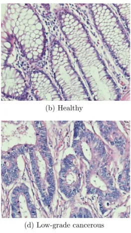
In a typical healthy colon tissue, there exist a large number of glands. Fig-ure 2.2a and FigFig-ure 2.2b show histopathological images of this kind of healthy colon tissues under microscope. The glandular structures indicated in Figure 2.1
(a) Healthy (b) Healthy
(c) Low-grade cancerous (d) Low-grade cancerous
(e) High-grade cancerous (f) High-grade cancerous
Figure 2.2: Histopathological images of colon tissues. These tissues are stained with the hematoxylin-and-eosin technique, which is a routinely used staining procedure in histopathology.
are easily perceived in these images. In the case of colon adenocarcinoma, these glandular structures are deformed, and eventually destroyed as the disease devel-ops. In the inception phase of the development of cancer, the spatial distribution of epithelial cells looks similar to those of a normal tissue, where the glandular structures are well to moderately differentiated. Figure 2.2c and Figure 2.2d show sample images from this kind of colon tissues, which are classified as low grade cancerous. Further development of cancer introduces a higher level of distortion to the tissue, causing the tissue components turn into a poorly differentiated dis-tribution and glandular structures totally disappear. Figure 2.2e and Figure 2.2f show sample images of this kind of colon tissues, which are classified as high grade cancerous.
A pathologist visually inspects biopsy specimens to determine the existence of malignant tumors in a tissue and their grades. Histopathological examination provides valuable information for the pathologist [14], however, the accuracy of his/her decisions significantly relies on his/her expertise. Based on the experience, histopathological examination may introduce considerable degrees of inter- and intra-observer variability. Besides, this variability may affect the selection of an appropriate treatment method.
2.2
Computer Aided Diagnosis and Grading of
Cancer
The observer variability involved in histopathological examination reveals the need of quantitative methods for cancer diagnosis and grading that reduce the subjectivity of the experts. In literature, numerous studies have been proposed to provide computer aided image analysis frameworks that make use of mathematical models for tissue representation. Computational methods in this context can be grouped into three; morphological, textural, and structural. This section provides information about these computational methods.
2.2.1
Morphological Methods
Cancer also causes changes in the geometric structure of cellular components. The degree of this change may indicate the malignancy of tumor. Morphological approach relies on the shape and size characteristics of its nuclear components to represent a tissue [104, 48, 88, 86]. To this end, local features of individual cell nuclei such as area, perimeter, roundness, and compactness are defined. To de-scribe the whole tissue, the average and standard deviation of these local features are computed.
Morphological approach is employed for the diagnosis and grading of different types of cancer. Street et al. [88] and Wolberg et al. [106] made use of morpho-logical features of breast cell nuclei to obtain quantitative information about the breast tissue. Guillaud [52] also proposed to use nuclear morphometry in the diagnosis of cervical intraepithelial neoplasia. Such morphological featuers are also used to quantify different tissue components. For example, Doyle et al. [37] focused on morphological features of glandular structures in a prostate tissue to achieve an automated diagnosis framework. Anderson et al. [6] also made use of morphological features of glandular tissue components for discriminating malignant and benign tumors in a breast tissue.
2.2.2
Textural Methods
Texture analysis is a widely used method in image processing applications. The aim of this approach is to extract distinguishing and descriptive features from images for characterizing their textures. These features include first order statis-tical features such as mean and variance, which are related to values of individual pixels, and second order statistical features such as correlation and contrast which account for co-occurrence or inter-dependency of pixel pairs.
2.2.2.1 Intensity Based Features
Intensity based features are used for describing pixel level characteristics of im-ages. To this end, gray level or color histograms of intensity values and densito-metric features are employed. Properties of these features such as mean, standard deviation, kurtosis, and skewness are computed to obtain first order statistical information about the texture of tissues.
In literature, there have been less number of studies that employ intensity based image features for the automated diagnosis and grading of cancer. Nev-ertheless, these features are used together with other image features to improve quantitative power of proposed representations. Wiltgen [105] used gray level histograms in combination with co-occurrence features for classification of be-nign common nevi and malignant melanoma. Weyn et al. [101] employed optical densities of nuclear tissue components in the quantification of breast tissue im-ages. The same group [104] used features obtained from densitometric properties of nuclear tissue components together with morphological and structural image features in the diagnosis and prognosis of malignant mesothelioma.
2.2.2.2 Co-occurrence Matrices
One of the most commonly used methods in texture analysis is co-occurrence matrices. Haralick [58] first proposed to use gray level co-occurrence matrices for the definition of textural image features. The values of a co-occurrence matrix represent the frequencies of pixels occurring in a relative distance to each other, one having the intensity value i and the other having the intensity value j. For a gray level image I with a size of w× h, a co-occurrence matrix M with relative distance d (x, y) is defined as follows:
M (i, j)d(x,y)= w ∑ p=1 h ∑ q=1 1, if I (p, q) = i and I (p + x, q + y) = j 0, otherwise (2.1)
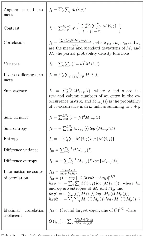
Angular second mo-ment f1 = ∑ i ∑ jM (i, j) 2 Contrast f2 = ∑Ng−1 n=0 n2 { ∑Ng i=1 ∑Ng j=1M (i, j) |i − j| = n } Correlation f3 = ∑ i ∑ j(ij)M (i,j)−µxµy σxσy , where µx, µy, σx, and σy
are the means and standard deviations of Mx and
My the partial probability density functions
Variance f4 = ∑ i ∑ j(i− µ) 2 M (i, j)
Inverse difference mo-ment f5 = ∑ i ∑ j 1 1+(i−j)2M (i, j) Sum average f6 = ∑2Ng
i=2 iMx+y(i), where x and y are the
row and column numbers of an entry in the co-occurrence matrix, and Mx+y(i) is the probability
of co-occurrence matrix indices summing to x + y
Sum variance f7 =
∑2Ng
i=2 (i− f8)2Mx+y(i)
Sum entropy f8 =−
∑2Ng
i=2 Mx+y(i) log{Mx+y(i)}
Entropy f9 =−
∑
i
∑
jM (i, j) log{M (i, j)}
Difference variance f10=
∑Ng−1
i=0 i2Mx−y(i)
Difference entropy f11=−
∑Ng−1
i=0 Mx−y(i) log{Mx−y(i)}
Information measures f12= maxhxy{hx,hy}−hxy1
of correlation f13= (1− exp [−2 (hxy2 − hxy)])1/2
hxy = −∑i∑jM (i, j) log (M (i, j)), where hx
and hy are entropies of Mx and My, and
hxy1 =−∑i∑jM (i, j) log{Mx(i) My(j)}
hxy2 =−∑i∑jMx(i) My(j) log{Mx(i) My(j)}
Maximal correlation
coefficient
f14= (Second largest eigenvalue of Q)1/2 where
Q (i, j) =∑k M (i,k)M (j,k)Mx(i)My(j)
The entries of co-occurrence matrices are not usually used directly as image features. Instead, a number of representative features are extracted from these co-occurrence matrices. Table 2.1 lists the definitions of the co-occurrence matrix features proposed by Haralick [58].
In general, co-occurrence matrices are computed from gray level intensities as first described by Haralick. However, in literature, there are a number of studies that use co-occurrence matrices computed from color images. Features extracted from these color co-occurrence matrices are also used for representing the image texture [83, 84]. Co-occurrence matrices are sensitive to rotation, and thus, they are generally computed using varying offset sets, such as 0, π/4, π/2, 3π/4, and the resulting co-occurrence matrices are combined to achieve rotation invariance [17, 38, 82].
Co-occurrence matrices are also proposed to be used in quantifying histopatho-logical images of different types of tissues [57, 102, 104, 17, 37]. Esgiar et al. [38] used co-occurrence features for automated categorization of normal and cancerous colonic mucosa. Wiltgen et al. [105] employed co-occurrence matrices to describe texture characteristics of histopathological images of skin tissues. Co-occurrence features have also been employed for the quantification of chromatin texture of cell nuclei [99, 101, 103].
2.2.2.3 Gray Level Run Length Matrices
Gray level run length method, defined by Galloway [45], is another textural ap-proach that provides higher order statistical information [92]. An entry M (i, j) of a gray level run length matrix M is defined as the number of sequences of pixels that have the gray level intensity value i and are of length j. Galloway first defined five statistical features on gray level run length matrices: short run emphasis, long run emphasis, gray level nonuniformity, run length nonuniformity, and run percentage [45]. Chu et al. [18] then extended these features defining two additional features: low gray level run emphasis and high gray level run em-phasis. Table 2.2 provides a list of these features. In this table, n is the number
Short run emphasis n1 ∑Gi ∑Rj M (i,j)j2
Long run emphasis n1 ∑Gi ∑Rj M (i, j) j2
Gray level nonuniformity n1 ∑Gi=1(∑Rj=1M (i, j)
)2
Run length nonuniformity n1 ∑Rj=1(∑Gi=1M (i, j)
)2
Run percentage np
Low gray level run emphasis n1 ∑Gi=1∑Rj=1 M (i,j)i2 High gray level run emphasis n1 ∑Gi=1∑Rj=1M (i, j) i2
Table 2.2: Gray level run length features.
of rows and p is the number of pixels in the image. Furthermore, Dasarathy et al. [24] defined another four features on gray level run length matrices measuring the joint statistics of gray levels and run lengths.
Gray level run length method has also a considerable number of applications in automated diagnosis and grading of different types of cancer [57, 104, 103]. Doyle et al. [36] employed run length features together with co-occurrence features for the quantification of breast tissues. Albertgensen et al. [4] made use of these features for quantifying images of liver tissues. Moreover, Weyn et al. [103] and Bibbo et al. [10] used run length features for representing the chromatin texture of nuclei in colon epithelium for the classification of normal and cancerous colon tissues.
2.2.2.4 Multi Resolution Wavelets
Multi resolution wavelets has also a considerable amount of interest in the lit-erature of texture analysis. Wavelet analysis is a mathematical method used
for extracting information from data signals, including audio signals and images. Wavelets are functions that are used for representing data signals by dividing them into components of different scales [49, 25]. In this decomposition process, which is named wavelet transform, each resulting component of the analyzed signal is studied with a resolution that matches to its scale [26].
Wavelet transforms are divided into two groups which are Continuous Wavelet Transforms (CWT) and Discrete Wavelet Transforms (DWT) respectively. Use of wavelets in multiple scales allows achieving multi-scale representations which increases the effectiveness of the method. Features obtained from these multi-wavelets such as short support, orthogonality, symmetry, and vanishing moments are known to be useful in image processing [3, 89, 95]. Wavelet analysis have a wide range of applications in literature, especially in the fields of image com-pression [7, 15, 23, 50, 61, 79] and image enhancement [73, 76]. Multiwavelet analysis method has also been employed in computerized diagnosis and grading of different types of cancers [91, 27, 101, 62, 104].
2.2.2.5 Image Fractals
Another textural method for image analysis is fractal geometry. Defined by Man-delbrot [71], a fractal is a geometrical shape which can be split into smaller parts, each of which looks identical to the whole. This method focuses on computing the fractal dimension of images, which gives an estimation of how a fractal appears to fill space as it is zoomed out.
Widely used method for computing fractal dimension is the box-counting
method. According to this method, fractal dimension D, also known as
Minkowski-Bouligand dimension [13], is defined in Equation 2.2 where N (ϵ) is the number of self-similar structures of diameter ϵ necessary to cover the structure.
D = lim
ϵ→0
log N (ϵ)
log 1ϵ (2.2)
Fractal geometry concept has been applied to analyze numerous textures in
quantification of different types of tissues [106, 34, 16, 8, 39].
2.2.3
Structural Methods
Structural approach has been employed by a large number of studies in medical image analysis, in addition to its various applications in other fields of image pro-cessing. Structural methods characterize a tissue using the spatial distribution and neighborhood properties of its cellular components. To this end, representa-tive graphs are constructed on these components, and a set of local and global features that provide quantitative information about tissues are computed.
Previous studies have proposed to use a number of different methods for con-structing their graphs. Commonly used methods are Delaunay triangulations and their corresponding Voronoi diagrams, minimum spanning trees, Gabriel’s graphs, and probabilistic graphs. These graph generation methods are summa-rized in the following subsections. Regardless of the methods, similar structural features have been extracted. A large number of these graph features are com-mon for different types of graphs, and they are used by a majority of structural representations. Besides, features specific to particular graphs are also proposed. The common local and global graph features that are used by different structural methods are given in Table 2.3. In this table, it is also indicated which features can be used by which methods. Structural approaches employ these local and global graph features for the quantification of tissue images. First order statistics of local graph features such as mean and standard deviation are also used as global features of graph based representations.
2.2.3.1 Delaunay Triangulation
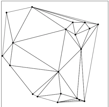
Delaunay triangulation is a commonly used graph generation method for modeling a wide range of concepts in different fields of science [41]. It was defined by Boris Delaunay [28], whose name was given to the method after his definition in 1934. Delaunay triangulation of a point set P in two dimensional space is defined as the
Feature Graph Category Area VD, DT Roundness VD Aspect ratio VD Circularity VD Number of sides VD Edge lengths DT, MST, GG Degree of nodes DT, MST, GG, PG
Distance to the nearest neighbor DT, MST, GG
Fractal dimension MST
Size ratio of giant connected component to graph PG
Eccentricity DT, MST, GG, PG
Clustering coefficient DT, MST, GG, PG
Shortest paths between nodes DT, GG, PG
Diameter DT, GG, PG, MST
Table 2.3: Structural features obtained from different graph based representa-tions: Voronoi diagrams (VD), Delaunay triangulations (DT), Gabriel’s graphs
(GG), minimum spanning tree (MST), and probabilistic graphs (PG).
set of triangles where each triangle conforms to the condition that there exist no point in the interior of the circle passing through the edge points px, py, pz ∈ P
of the triangle. The condition of Delaunay guaranties that each triangle of the triangulation has an empty circumcircle and maximizes the minimum interior angles of the triangles. Figure 2.3 shows a sample Delaunay triangulation of 20 random points in two dimensional Euclidean space.
Delaunay triangulations have been used to build structural representations of various tissues for automated cancer diagnosis and grading. In [65], an auto-mated framework that make use of Delaunay triangulations for grading of cervical intraepithelial neoplasia is proposed. Guillaud et al. [52] proposed to use Delau-nay features for quantification of cervical tissues. Doyle et al. [36] proposed an automated diagnosis and grading method for breast cancer that also employs Delaunay triangulations.
Figure 2.3: Delaunay triangulation of 20 random points in 2 dimensional Eu-clidean space.
2.2.3.2 Voronoi Diagrams
Voronoi diagrams, which are dual graphs of Delaunay triangulations, are also widely used in structural image analysis methods. The idea lying under Voronoi diagrams was first emphasized by Descarts [31, 74] when he was trying to model the solar system, claiming that the solar system consists of vortices, the convex regions around the stars. This concept has independently emerged in various fields including biology, physiology, chemistry, and physics. It has been used with different names in these field, such as medial axis transform in biology and physiology, Wigner-Seitz zones in chemistry and physics, domains of action in crystallography, and Thiessen polygons in meteorology and geography [78].
First formal definitions were proposed by the mathematicians Dirichtlet [32] and Voronoi [97, 98], with the names Dirichtlet tessellation and Voronoi diagram which have become the standard names in literature. Voronoi diagram is defined as the decomposition of a regular plane of n points into convex polygons called Voronoi regions such that each point inside a Voronoi region is closer to the
Figure 2.4: Voronoi diagram of the point set used in Figure 2.3.
origin point of that region than any other point in the plane. Voronoi diagrams are dual graphs of Delaunay triangulations, and they are generally used together in structural methods. Figure 2.4 shows the corresponding Voronoi diagram of the Delaunay triangulation given in Figure 2.3.
In literature, there are a number of studies that make use of Voronoi dia-grams for quantification of histopathological images [90, 80]. Weyn et al. [102] proposed to use Voronoi diagrams to develop an automated method for diagnosis and grading of malignant mesothelioma. Doyle et al. [37] used Voronoi diagrams to extract structural image features from breast tissue images. Morover, a com-parative study of morphological, textural, and structural image features that use Voronoi diagrams is provided in [104].
2.2.3.3 Gabriel’s Graph
Another type of graph representations that is used for modeling the neighborhood characteristics of cellular components of tissues is Gabriel’s graphs. This graph
Figure 2.5: Gabriel’s graph of the point set used in Figure 2.3.
generation method was proposed by Gabriel et al. [44]. Given a point set P , two points pi, pj ∈ P are said to be Gabriel neighbors if and only if the circle having
the line segment [pipj] as its diameter has no other point pk ∈ P in its interior.
And the set of edges connecting the points that conform this property of Gabriel neighborhood is called a Gabriel’s graph. A sample Gabriel’s graph generated using point set of Figure 2.3 is presented in Figure 2.5. Gabriel’s graphs are subgraphs of Delaunay triangulations [77]; this can be observed from Figure 2.3 and Figure 2.5.
2.2.3.4 Minimum Spanning Tree
Although it has less applications, minimum spanning trees are also employed for improving the graph based representations. A minimum spanning tree T of a weighted undirected graph G is the subgraph of G which has the minimum total weight among all possible connected subgraphs of G which have n− 1 edges between n nodes of the graph without cycles and self loops. Figure 2.6 shows a minimum spanning tree of the Delaunay triangulation presented in Figure 2.3.
Figure 2.6: Minimum spanning tree of the Delaunay triangulation given in Figure 2.3.
Minimum spanning trees are used in conjunction with aforementioned graph based representations for automated cancer diagnosis and grading. Therefore, minimum spanning trees are obtained from Delaunay triangulations and a set of global features based on edge lengths are extracted. First order statistics such as mean, standard deviation, and kurtosis of these features are computed for quantifying tissues [104]. Weyn et al. [102] used minimum spanning trees in the automated diagnosis of malignant mesothelioma. Doyle et al. [36] and Guillaud et al. [52] also employed minimum spanning trees to quantify images of cervical tissues. Choi et al. [17] proposed to use minimum spanning trees in their comparative study on object-based, textural, and structural methods in the classification of bladder cancer.
2.2.3.5 Probabilistic Graphs
In probabilistic graphs edges between nodes are probabilistically assigned accord-ing to the distance between the nodes. In this method, the edge density of a graph is controlled with a probability function that can be defined in different ways. For
Figure 2.7: Probabilistic graph generated on the point set given in Figure 2.3. Here, Equation 2.3 is used with α = 2 and r = 0.2.
example, in [30, 53], probabilistic graphs are constructed by using the following equation: E (u, v) = 1, if d (u, v)−α > r 0, otherwise (2.3)
In this equation, r is a random number between 0 and 1, and d (u, v) is the Euclidean distance between nodes u and v. Here α is used as a parameter for controlling the edge density of generated graphs. Figure 2.7 shows a sample probabilistic graph which is generated using the function given in Equation 2.3.
Probabilistic graphs have been employed for modeling a large number of do-mains such as social networks and the world wide web. In [53], a novel probabilis-tic graph generation method is proposed to model brain tumor. Local and global features computed from these graphs are used for characterizing cancerous brain tissue [53, 30]. Demir et al. [29] proposed to use augmented cell-graphs, that are undirected, weighted, and complete probabilistic graphs without self loops,
for automated diagnosis of cancer, where all possible edges between each pair of nodes are included in the graph, preventing the loss of any existing spatial information. In these graphs, edge weights are defined as the Euclidean distances between their end nodes. Furthermore, Gunduz-Demir [54] investigated the re-lation of different phases of cell-graphs with the malignancy of the cancer using graph evolution technique.
Methodology
In Chapter 2 we have described the computational methods that are proposed for developing computer aided image analysis tools. These tools can be employed in cancer diagnosis and grading processes to obtain quantitative information about the characteristics of tissues, and help reducing the subjectivity of pathologists. Therefore, proposed methods define mathematical representations of tissues with the use of morphological, textural, and structural features of histopathological images. Although these methods yield accurate results for diagnosis and grading of cancer, they mainly focus on nuclear characteristics of tissues, ignoring the role of other components in the tissue structure. In this thesis, we propose a novel structural representation for the quantification of different components of histopathological tissue images. In addition to nuclear tissue components, the proposed method considers different components of a tissue such as luminal and stromal regions. It takes spatial relationships and neighborhood properties of these components into account in making decisions.
The proposed method consists of the following four steps: (1) node identifica-tion, (2) edge identificaidentifica-tion, (3) feature extracidentifica-tion, and (4) classification. In the node identification step, image pixels are converted into Lab color space and then segmented into three sets corresponding to luminal, stromal, and nuclear regions. Subsequently, morphological operations are applied on each of these pixel sets for reducing noise and circular components are located on each region. These
K−means clustering Circle fitting RGB2Lab transformation Node Identification Edge labeling Edge Identification Delaunay triangulation Feature extraction Classification Histopathological image
components are considered as the graph nodes. In the next step, a graph is con-structed on these nodes making use of Delaunay triangulation, and the triangle edges are colored according to the component types of their end nodes. Then, a set of graph features is computed from the constructed color graph that is used in the classification step. Figure 3.1 shows a shematic representation of the pro-posed approach. Next subsections provide detailed descriptions and outputs of the steps of the proposed color graph approach.
3.1
Node Identification
Color graph approach takes all components of a tissue into account to effectively quantize its histopathological image. To this end, nuclear, stromal, and luminal components of a tissue are mapped to graph nodes. To perform this mapping, histopathological images should be segmented into its cytological components. The ideal way of this segmentation is to identify the exact boundaries of each component. However, in a typical histopathological image, there could be stain-ing and sectionstain-ing related problems, includstain-ing the existence of touchstain-ing and over-lapping components, lack of dark separation lines between a component and its surroundings, inhomogeneity of the interior of a component, and presence of stain artifacts in a tissue [48]. This complex nature of a histopathological image scene leads to a difficult segmentation problem even for the human eye. Therefore, the proposed approach approximately represents the tissue components with three sets of circular primitives corresponding to nuclear, stromal, and luminal regions. The centroids of these tissue components are considered as the node locations in constructing a color graph.
3.1.1
Clustering with K-means
To identify the component of a tissue, pixels of its histopathological image are seg-mented into three clusters using the k-means algorithm. The number of clusters is particularly selected as three since there are mainly three color groups in the
histopathological image of a tissue that is stained with hematoxylin-and-eosin. These colors are purple, pink, and white, which typically correspond to nuclear, stromal, and luminal components, respectively.
Before clustering, image pixels are converted into Lab color space to take ad-vantage of luminance components of pixel values. Lab color space is a commonly preferred color space over RGB color space in image processing applications. It is a color-opponent space, which approximates the visual perception of human eye. Its dimensions L, a, and b correspond to luminance, greenness-redness, and blueness-yellowness components respectively. This color space improves image analysis methods since its L component closely matches human perception of lightness [47].
The k-means algorithm [70], which is one of the most commonly used unsuper-vised learning algorithms that partitions an N dimensional data into k subsets, is used for segmentation. This algorithm attempts to assign each data point to a cluster Si, minimizing the within cluster sum of squares or squared error function
E given in Equation 3.1. E = k ∑ i=1 ∑ j∈Si ∥ xj − ci ∥2 (3.1)
In Equation 3.1, the term ∥ xj− ci ∥ is a distance measure between the
centroid ci and the observation xj assigned to the cluster Si. In this study, we
use k-means implementation of Matlab with Euclidean distance as the distance measure for clustering. With the utilization of k-means algorithm, the centroids of clusters are computed and types of these centroids are determined according to the values of their L component. This determination depends on the idea that lower values of L component correspond to darker colors, and higher values correspond to brighter colors. Thus, we label the pixels that have the lightest centroid as luminal pixels since luminal regions of a tissue correspond to white colored pixels in the histopathological image. Similarly, pixels that have the darkest centroid are labeled as nuclear pixels since nuclear tissue components are the darkest colored regions in images. And the remaining pixels are labeled as
(a) Healthy (b) Healthy
(c) Low-grade cancerous (d) Low-grade cancerous
(e) High-grade cancerous (f) High-grade cancerous
Figure 3.2: Pixel clusters of histopathological images given in Figure 2.2 that are obtained using k-means.
stromal pixels. Figure 3.2 shows resulting images of the clustering process.
At the end of this step, we obtain three binary images corresponding to nu-clear, stromal, and luminal regions, respectively. These images are preprocessed to reduce the noise that arises from the incorrect clustering of pixels. To this end, on the pixels of these images, closing and opening operators with a square structuring element of size 3 are applied sequentially. Closing operation removes noisy pixels and fills small holes, whereas opening removes small objects from the images. After this preprocessing, these binary images are used as pixel masks on nuclear, luminal, and stromal regions.
3.1.2
Circle Fitting
After clustering and preprocessing of histopathological images, we obtained three images each of which consists of pixels that belong to nuclear, luminal, and stro-mal regions. This segmentation process discriminates different types of tissue components. However, it still does not eliminate the difficulty of identifying the exact boundaries of individual tissue components. Thus, segmentation of these components remains as a challenging problem.
In order to overcome this difficulty, the proposed approach approximately represents a tissue component with a circle object instead of identifying its exact boundary. To perform this task, it employs a heuristic method called circle
fit-ting [94, 55] for defining circular primitives on binary images obtained in the
pre-vious step. Given a particular connected component of the image, the algorithm first locates a circle on the pixels of this component, which has the largest diame-ter conforming that it does not exceed the borders of the component. The pixels covered by the located circle are labeled. The algorithm then locates smaller circles on the unlabeled pixels of the connected component conforming that the circles inside the component do not overlap each other and do not exceed the borders of the component. The algorithm iteratively locates smaller circles on unlabeled pixels as far as the areas of generated circles reach to a value smaller than a predefined area threshold. This iterative procedure continues until each
(a) Healthy (b) Healthy
(c) Low-grade cancerous (d) Low-grade cancerous
(e) High-grade cancerous (f) High-grade cancerous
Figure 3.3: Circular primitives that are obtained by applying the circle fitting algorithm to pixel clusters of images given in Figure 3.2.
connected component of the image is processed.
Using the aforementioned method, pixel masks of nuclear, stromal, and lumi-nal regions are transformed into circular primitives that approximately represent these tissue components. The motivation lying under the idea of using circular objects is that cytological components of the colon tissue components typically have curvy boundaries and circles are efficiently located on a set of pixels. This approach effectively maps a tissue component to a circular primitive; however, it may also split a tissue component into more than one circle especially those having elliptical shapes. Figure 3.3 shows the circles that are obtained by trans-forming the images given in Figure 3.2 into circular primitives with the use of the circle fitting algorithm.
At the end of circle fitting step, we obtain three sets of circles corresponding to different types of tissue components. The coordinates of the centroids and types of these circles are used the next step of the proposed approach for defining the edges of the graph.
3.2
Edge Identification
In the previous section, we have identified the locations of circular primitives as graph nodes. The next step of the proposed approach assigns edges between these nodes to build a graph model that represents the underlying tissue image. For this purpose, it constructs a Delaunay triangulation on these nodes.
As mentioned in Section 2.2.3, Delaunay triangulation method is a commonly used structural method for automated analysis of histopathological images. The definition of Delaunay triangulation models the spatial relationships of nodes in a graph. This characteristic of Delaunay triangulation makes it suitable for representing organizational structures of tissues.
Previous studies on structural tissue analysis commonly proposed to construct Delaunay triangulations only on the nuclear tissue components focusing on the
Green : Luminal-luminal edge
Red : Stromal-stromal edge
Blue : Nuclear-nuclear edge
Yellow : Luminal-stromal edge
Cyan : Luminal-nuclear edge
Magenta : Stromal-nuclear edge
Table 3.1: List of colors that are used for labeling triangle edges.
distribution of cell nuclei in tissues. Although these mathematical representations provide representative information for some tissue types, they may not efficiently represent tissues where cytological components other than nuclei also reflect the structural characteristics of the tissue.
On the other hand, the proposed approach builds a Delaunay triangulation on three types of nodes corresponding to nuclear, stromal, and luminal tissue components. Then, it labels the edges of the resulting graph according to the types of their end nodes. As there are three different types of nodes, edges are colored with one of the six colors that are given in Table 3.1. Figure 3.4 shows the color graphs that are constructed on the circles given in Figure 3.3.
In literature, there have been a number of methods for constructing Delaunay triangulations [42, 43, 51]. In this study, we have employed a Matlab function that uses the Qhull [9] algorithm for computing Delaunay triangulation.
3.3
Feature Extraction
In order to quantify histopathological images, three groups of global graph fea-tures that are commonly used by structural image analysis methods are computed from constructed color graphs. These are average degree, average clustering co-efficient, and diameter. Additionally, we aim to introduce the color information into the computations of these graph features. The definitions of these features are given in the following subsections.
(a) Healthy (b) Healthy
(c) Low-grade cancerous (d) Low-grade cancerous
(e) High-grade cancerous (f) High-grade cancerous
Figure 3.4: Color graphs that are generated from the graph nodes given in Fig-ure 3.3 and that are colored with one of the six colors given in Table 3.1 depending on the component types of their end nodes.
3.3.1
Average Degree
In graph theory, the degree of a node is defined as the number of its adjacent neighbors. The average degree of a graph is the mean of the degrees computed for every node in the graph. In this study, seven degrees are computed for a single node using the following definitions:
• Degree: Given a color graph G (N, E), the degree di of node i ∈ N is the
total number of its edges, regardless of their colors. This is a common feature that is used to quantify the local connectivity properties of a graph.
• Color degree: Given a color graph G (N, E), the color degree dic of node
i∈ N is the total number of its edges that are of color c. For a particular
node of the color graph, we define six color degrees as there exits six types of edges in the graph connecting three types of nodes. This feature is used for quantifying the local connectivity of different types of graph nodes.
Taking the averages of these local graph features, seven average degrees are obtained for an individual color graph.
3.3.2
Average Clustering Coefficient
Average clustering coefficient also provides information about the connectivity of a graph [35]. It indicates the density of connections in the neighborhood of a node. For an individual color graph, four clustering coefficients are computed using the following definitions:
• Clustering coefficient: Clustering coefficient of a node is defined as the
ratio of the number of existing edges over the number of all possible edges
between its neighbors. Clustering coefficient Ci of node i is computed as
follows:
Ci =
2di· Ei
di· (di− 1)
where di is the degree of i and Ei is the number of existing edges between
its neighbors.
• Color clustering coefficient: The color clustering coefficient of a node is
de-fined to quantify the clustering information of nodes of the same component type. For this purpose, a colored clustering coefficient is defined for each node considering only its neighbors of the same type. For instance, for a lu-minal component node, only the lulu-minal-lulu-minal edges are considered and a luminal clustering coefficient Cil is defined as
Cil = 2dil· Eil dil· ( dil− 1 ) (3.3)
where dilis the number of luminal neighbors of i and Eilis the number of
ex-isting edges between these neighbors. Similarly, color clustering coefficients
Cis and Cin are computed for stromal and nuclear component nodes.
Averaging the clustering coefficients over all nodes, four global features are obtained to quantify a color graph.
3.3.3
Diameter
The shortest path between two nodes u and v of a graph is defined as the minimum number of adjacent edges that have to be traveled from u to v. The diameter of a graph is the length of the longest of the shortest paths between any pair of graph nodes. Diameter is a global feature that indicates the size of the graph. In this work, seven diameters, one colorless and six color diameters, for a color graph are computed. The first diameter is computed without considering the edge colors such that adjacent edges in the computed paths may be of different types. The other six of the graph diameters are computed considering only the edges with a color of interest. For instance, the green diameter is the longest of the shortest paths between any pair of nodes that are reachable to each other using only the luminal-luminal (green) edges.
3.4
Classification
In Section 3.3, 18 dimensional feature vectors are defined for color graphs to quan-tify histopathological tissue images. In the last step of the proposed approach, these feature vectors are used by support vector machines to achieve classification.
3.4.1
Support Vector Machines
For an effective classification method, it is important to accurately classify not only the observed data but also the unknown data. Thus, it is necessary to se-lect the most appropriate boundary that will optimally separate the unpredicted data. Numerous parametric models that are based on the probability density estimations of classes are proposed for performing this task. Support vector ma-chines provide a non-parametric classification method that solves an optimization problem.
The support vector machine is a kernel-based supervised learning method that is used for classification and regression. The support vector machine algorithm was originally proposed as a linear classifier [21]. The algorithm aims to partition
data points of two classes in n dimensional space with an n − 1 dimensional
hyperplane. In general, there may be more than one hyperplane separating the data points. Figure 3.5a shows such possible separations of data points of two classes in two dimensional space. The fundamental idea of the algorithm is to find the separating hyperplane that maximizes the margin, which is the distance of the nearest data points in both data sets to the separating hyperplane. Figure 3.5b shows an optimal separation of data points in Figure 3.5a, which maximizes the margins. Data points that lie on the margins are called support vectors.
The original definition of support vector machines provides a linear classifi-cation model. However, it is not always possible to linearly separate data. For example, for the data points given in Figure 3.6a, it is impossible to locate a lin-ear boundary that totally separates two classes, which limits the effectiveness of support vector machines. On the other hand, extensions have been proposed to