Batch learning of disjoint feature intervals

H

n Ä·

'-Λ

;·:·ί

ii

■.··· ■

.^' ;:; ^

Щ

:·ί :> : ^ ^ ·ν '

*№' ii irii '.»k· ·%./ >i t. J .; Ä .1 .· ,!· « 0 «w' i-jii L:.. .. л' . ' ■

P: T H £ S

;3

DISJOINT FEATURE INTERVALS

A THESIS

SUBMITTED TO THE DEPARTMENT OF COMPUTER ENGINEERING AND INFORMATION SCIENCE AND THE INSTITUTE OF ENGINEERING AND SCIENCE

OF BILKENT UNIVERSITY

IN PARTIAL FULFILLMENT OF THE REQUIREMENTS FOR THE DEGREE OF

MASTER OF SCIENCE

by

Aynur Akku§

September, 1996

-м г> Й 35

Assoc; Prof. H ^ l Altav Güven:Altay Güvenir (Advisor)

I certify that I have read this thesis and that in my opinion it is fully adequate, in scope and in quality, as a thesis for the degree of Master of Science.

< ?^ t. Prof. Kemal Oflazer

I certify that I have read this thesis and that in my opinion it is fully adequate, in scope and in quality, as a thesis for the degree of Master of Science.

Approved for the Institute of Engineering and Science:

Prof. Mehmet ^i^ay

Director of Institute of Engineering and Science

BATCH LEARNING OF DISJOINT FEATURE INTERVALS

Aynur Akkuş

M.S. in Computer Engineering and Information Science Supervisor: Assoc. Prof. Halil Altay Güvenir

September, 1996

This thesis presents several learning algorithms for multi-concept descriptions in the form of disjoint feature intervals, called Feature Interval Learning algo­ rithms (FIL). These algorithms are batch supervised inductive learning algo­ rithms, and use feature projections of the training instances for the representci- tion of the classification knowledge induced. These projections can be general­ ized into disjoint feature intervals. Therefore, the concept description learned is a set of disjoint intervals separately for each feature. The classification of an unseen instance is based on the weighted majority voting among the local predictions of features. In order to handle noisy instances, several extensions are developed by placing weights to intervals rather than features. Empirical evaluation of the FIL algorithms is presented and compared with some other similar classification algorithms. Although the FIL algorithms achieve compa­ rable accuracies with other algorithms, their average running times are much more less than the others.

This thesis also presents a new adaptation of the well-known /s-NN clas­ sification algorithm to the feature projections approach, called A:-NNFP for k-Nearest Neighbor on Feature Projections, based on a majority voting on in­ dividual classifications made by the projections of the training set on each feature and compares with the /:-NN algorithm on some real-world and cirtifi- cial datasets.

Keywords: machine learning, supervised learning, inductive learning, batch

learning, feature projections, voting.

AYRIK ÖZNİTELİK BÖLÜNTÜLERİNİ TOPLU ÖĞRENM E

Aynur Akkuş

Bilgisayar ve Enformatik Mühendisliği, Yüksek Lisans Tez Yöneticisi: Doç. Dr. Halil Altay Güvenir

Eylül, 1996

Bu tezde öznitelik izdüşümlerine dayalı yeni öğrenme algoritmaları sunulmuş­ tur. Oznitelik Bölüntülerini Öğrenme (FİL) olarak isimlendirilen bu algorit­ malar toplu, denetimli ve türnevarımsal öğrenme yöntemlerini kullanırlar ve öğrenme örneklerinin öznitelik izdüşümlerini sınıflama bilgisini çıkarmak için kullanırlar. Bu izdüşümler ayrık öznitelik bölüntülerine genellenir. Böylece, öğrenilen kavram tanımları her öznitelik için ayrık öznitelik bölüntüleri şeklinde gösterilir. Daha önce görülmemiş bir örneğin sınıflandırması için her öznitelik tarafından bir ön sınıflandırma yapılır ve son sınıflama bu ön sınıflandırmaların ağırlıklı çoğunluk oylamasıyla belirlenir. Hatalı örnekleri tespit edebilmek için bölüntülere ağırlık verilerek bazı değişiklikler önerilmiştir. FİL algoritmalarının benzer sistemlerle uygulama sonuçları doğal ve yapay veri kümeleri üzerinde karşılaştırılmıştır. Bu algoritmaların doğruluk oranları dahci öncekilere yakın olmasına rağmen ortalama çalışma süreleri çok daha azdır.

Bu tezde literatürde yaygın olarak bilinen k en yakın komşu sınıflandırma algoritması (UNN) yeniden tanımlanmıştır ve UNNFP, öznitelik izdüşümleri üzerinde k en yakın komşu sınıflandırması, olarak isimlendirilmiştir. k-NNFP algoritmasında sınıflandırma her öznitelikten gelecek olan tahminler arasından çoğunluk oylaması yapılarak belirlenir. A;-NNFP ve fc-NN algoritmalarının karşılaştırılması doğal ve yapay veri kümeleri üzerinde yapılmıştır.

Anahtar Sözcükler: öğrenme, türnevarımsal öğrenme, toplu öğrenme, dene­

timli öğrenme, öznitelik izdüşümleri, oylama. iv

I would like to express rny gratitude to Assoc. Prof. H. Altay Güvenir due to his supervision, suggestions, and understanding throughout the development of this thesis.

I am also indebted to Assist. Prof. Kemal Oflazer and Assist. Prof. Ilyas Çiçekli for showing keen interest to the subject matter and accepting to read and review this thesis.

I cannot fully express my gratitude and thanks to Savaş Dayanik and my parents for their morale support and encouragement.

I would also like to thank to Bilge Say, Yücel Saygın, Gülşen Demiröz cind Halime Büyükyıldız for their friendship and support.

This thesis was supported by TUBITAK (Scientific and Technical Research Council of Turkey) under Grant EEEAG-153.

1 Introduction 1

2 Concept Learning Models 8

2.1 Exemplar-Based Learning 10

2

.

1.1

Instance-Based Learning (IBL)

11

2

.

1.2

Nested-Generalized Exemplars (NGE) 14

2.1.3 Generalized Feature Values... 16

2.2

Decision T r e e s ... 17

2.3 Statistical Concept L earn in g... 19

2.3.1 Bayes Decision Theory - Naive Bayesian Classifier (NBC) 20

2

.

3.2

Nearest Neighbor Classifiers (NN) 23

2.3.3 NN Classifier on Feature Projections ( N N F P ) ... 25

3 Feature Projections for Knowledge Representation 26

3.1 Classification by Feature Partitioning ( C F P ) ... 27

3.2 Classification with Overlapping Feature Intervals (COFI) . . . . 31

3.3.1 The A:-NNFP A lg o r it h m ... .36

3.3.2 Evaluation of the A:-NNFP A lg o rith m ... 40

3.3.3 D iscu ssion ...

45

3.4 Weighting Features in к Nearest Neighbor Classification on Fea­ ture Projections (A:-NNFP)... 46

3.4.1 The Weighted k-NNFP A lgorith m ... 47

3.4.2 Some Methods for Learning Feature W e ig h ts... 48

3.4.3 Experiments on Real-World D a ta s e ts ... 50

3.4.4 D iscu ssion ... 51

3.5 Summary 52 4 Batch Learning of Disjoint Feature Intervals 53 4.1 Basic D e fin it io n s ... 54

4.2 Description of the FIL A lgorithm s... 56

4.2.1 The FIl A lg o r ith m ... 56

4.2.2 The FI2 A lg o r ith m ... 64

4.2.3 The FI3 A lg o r ith m ... 65

4.2.4 The FI4 A lg o r ith m ...

68

4.3 Characteristics of FIL A lg orith m s... 69

4.3.1 Knowledge R epresentation... 72

4.3.2 Inductive L e a r n in g ... 73

4.3.4 Batch L e a r n in g ...

74

4.3.5 Domain Independence in Learning... 75

4.3.6 Multi-concept Learning... 76

4.3.7 Properties of Feature V a lu e s ... 76

4.3.8 Handling Missing (Unknown) Feature V alu es... 77

4.4 User In te rfa ce ... 77

4.5 S u m m a r y ... 82

5 Evaluation of the FIL Algorithms 83 5.1 Complexity A n a ly s is ... 83

5.2 Empirical Evaluation of the FIL A lg o r it h m s ... 85

5.2.1 Testing M e th o d o lo g y ... 85

5.2.2 Experiments with Real-World D a ta se ts... 87

5.2.3 Experiments with Artificial D a t a s e t s ... 89

5.3 S u m m a r y ... 94

6 Conclusions and Future Work 95

A Real-World Datasets 105

2.1

Classification of exemplar-based learning models. 10

2.2

An example concept descrij^tion of the EACH algorithm in a domain with two features... 16

3.1 Construction of intervals in the CFP algorithm: (a) after i\ is processed, (b) after

¿2

is processed, (c) after

¿3

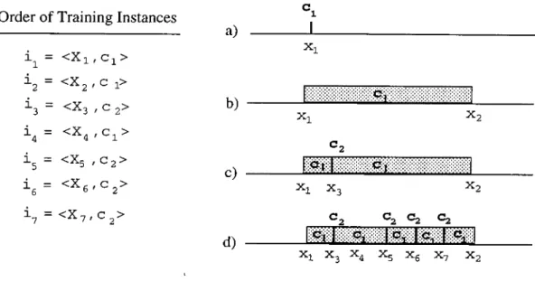
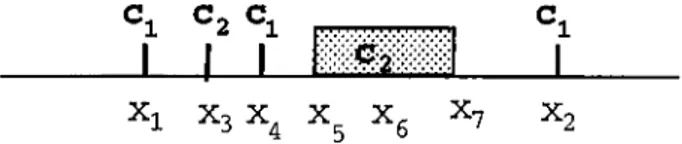
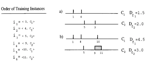
is processed, (d) after all training instances are processed... 28

3.2

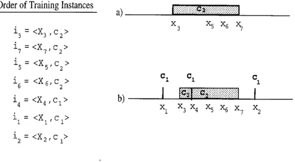
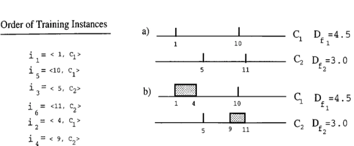
Construction of intervals in the CFP algorithm by changing the order of the training instances. Note that here the same set of instances in Figure 3.1., but in a different order, is used as the training set: (a) after ¿

3

,^

7

,

¿5

and are processed, (b) after alt

instances are processed. 30

3.3 Construction of the intervals in the FIL algorithms with using the same dataset as used in Figure 3.1 and Figure 3.2. 31

3.4 An example of construction of intervals in the COFI algorithm: (a) after ¿

1

, ¿

2

,

¿3

and

¿4

are processed, (b) after

¿5

and are processed... 32

3.5 An example of construction of intervals in the COFI algorithm using the same set of training instances as in Figure 3.6, but in a different order: a) after ¿

1

, ¿

5

, ¿

3

, and ie are processed, b) after

¿2

and

¿4

are processed. 34

Figure 3.5...

35

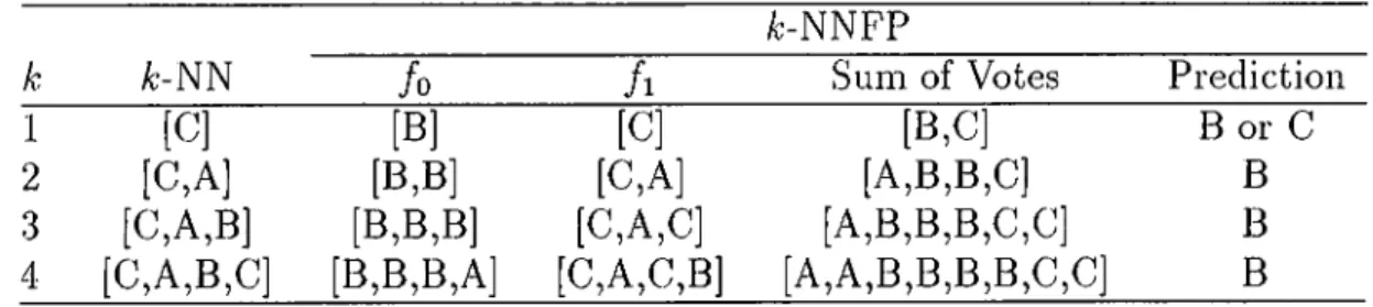
3.7 Classification in the A:-NNFP algorithm. 37

3.8 A sample training dataset and a test instance... 39

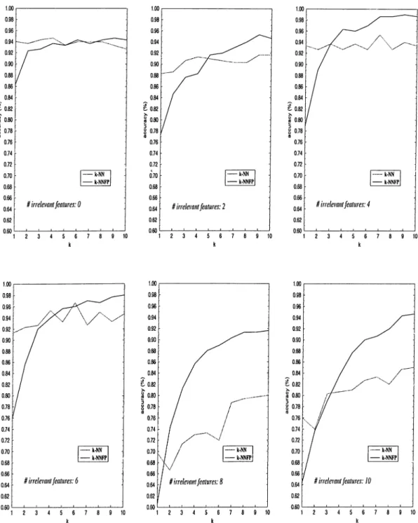
3.9 Comparison of ¿-NN and A:-NNFP on artificial datasets for in­ creasing value of k. In all datasets there are 4 relevant features, 3 classes and 100 instances for each class. The accuracy results are obtained by 5 way cross-validation... 44

3.10 Classification in the weighted A:-NNFP algorithm... 48

3.11 Homogeneous distribution on a feature d im e n s io n ... 49

3.12 Heterogeneous distribution on a feature dimension 49

4.1 An example for an interval. 54

4.2 An example for a point interval. 55

4.3 An example for a multi-class point... 55

4.4 A Sam

2

Dle Training Set and Feature Projections on Each Feature

Dimension 58

4.5 Construction of feature intervals in the FIl algorithm. 59

4.6 Training process in the FIl algorithm. 60

4.7 An example for classification in the FIl algorithm... 61

4.8 Classification process in the FIl algorithm... 63

4.9 An Example for an incorrect classification in the FIl algorithm

that leads to the EI

2

Algorithm. 64

4.10 Generalization of intervals in the FI

2

algorithm...

66

4.12 Construction of feature intervals in the FI3 algorithm. 67

4.13 An example for classification in the FI3 algorithm. 69

4.14 Training process in the FI3 algorithm. 70

4.15 Classification process in the FI3 algorithm... 71

4.16 Normalization of interval weights in the FI4 algorithm... 71

4.17 An example of classification in the FI4 algorithm. 72

4.18 An example for the information provided to the FIL algorithms. 77

4.19 Intervals of iris domain on the first feature. 78

4.20 Intervals of iris domain on the second feature... 79

4.21 Intervals of iris domain on the third feature... 80

4.22 Intervals of iris domain on the fourth feature. 80

4.23 Feature intervals constructed by the FIl algorithm for the iris

dataset. 81

5.1 Accuracy results of the FIL, CFP, NBC, A:-NN, ¿-NNFP algo­ rithms on domains with irrelevant attributes... 90

5.2

Accuracy results of the FIL, CFP, NBC, ¿-NN, A;-NNFP algo­ rithms on domains with increasing noise level... 92

5.3 Accuracy results of the FIL, CFP, NBC, A;-NN and A:-NNFP algorithms on domains with increasing ratio of missing feature

values. 93

3.1 For the test instance (< 5,5 > ) in Figure 2 the /j-NN classifica­ tion, kBag values and final prediction of the A:-NNFP algorithm. 39

3.2

Accuracy (%) and average running time (msec) of the A;-NNFP

algorithm on real-world datasets. 42

3.3 Accuracy (%) and average running time (msec) of the A;-NN

algorithm on real-world datasets. 42

3.4 The average time (in msec) required to train with 80% and test with the

20

% of the artificial datasets for increasing number of features... 42

3.5 Accuracies (%) of the ¿-NNFP (N) and its weighted versions us­ ing homogeneneous feature projections (HFP) and single feature accuracy (SFA) feature weighting methods... 51

5.1 Accuracy results (%) of the FIL algorithms on real-world datasets. SFA-FIx and HFP-FIx show the weighted versions of the FIl and FI2 algorithms... 87

5.2

Accuracy results (% ) of the FI4, NBC, CFP, ¿-NNFP and k-NN

algorithms on real-world datasets.

88

5.3 The Average Time (msec) required for the FIL, NBC, CFP, k-NN and fc-k-NNFP algorithms on real-world datasets... 89

A .l Comparison on some real-world datasets...105

CFP COFI Cг C4 C4.5 D j Deh E E j h 9 EACH FIL FIl FI2 FI3 FI4 GA-CFP H E f H f flower Hf,upper HFP IBL IB l IB2 IB3 IB4 IB5 ID3 k k

: Classification by Feature Partitioning

Classification by Overlapping Feature Intervals Label of the ¿th class

Decision tree algorithm Decision tree algorithm

Generalization distance for feature / in the COFI algorithm Euclidean distance between example E and exemplar H An example

/t h feature value of the example E jth feature

Generalization ratio

Exemplar-Aided Constructor of Hyperrectangles Feature Interval Learning Algorithms

Feature Interval Learning Algorithm Feature Interval Learning Algorithm Feature Interval Learning Algorithm Feature Interval Learning Algorithm Hybrid CFP Algorithm

Hyperrectangle

/t h feature value of the exemplar H

Lower end of the range for the exemplar H for feature / Upper end of the range for the exemplar H for feature / Homogeneous Feature Projections feature Weighting Method Instance-based learning

Instance-based learning algorithm Instance-based learning algorithm Instance-based learning algorithm Instance-based learning algorithm Instance-based learning algorithm Decision tree algorithm

Number of classes in the dataset no of neighbors in A:-NN and ^-NNP’P

m m axj m in j n NBC NGE NN P ( x h i) P{Wc) P{wc\x.) R ( a i , x ) SEA T2 X Xi W f Wh IR

Л

X{ai,Wj)

Number of training instances Maximum value for the feature / Minimum value for the feature / Number of features in the dataset Naive Bayesian Classifier

Nested-Generalized Exemplars Nearest Neighbor Algorithm

Conditional probability density function for x conditioned on given Wj Prior probability of being class c for an instance

The posterior probability of an instance being class c given the observed feature value vector x

Conditional risk

Single Feature Accuracy Feature Weighting Method

Agnostic РАС learning decision tree algorithm with at most two levels Instance vector

Value vector of Rh instance Weight of feature /

Weight of exemplar H

System whose input is training examples and output is 1-rule Weight adjustment rate of the CFP algorithm

Loss incurred for taking action ai when the state of nature is Wj

Introduction

Machine learning has played a central role in artificial intelligence since 1980’s, especially in modeling behavior of human cognition and human thought pro­ cesses for problem solving strategies. The studies in machine learning suggest computational algorithms and analyses of such algorithms that suggest expla­ nations for capabilities and limitations of human cognition. Learning can be described as increasing the knowledge or skills in accomplishing certain tasks [13]. The learner applies inferences in order to construct an ajDpropriate repre­ sentation of some relevant reality.

One of the fundamental research problems in machine learning is how to learn from examples since it it usually possible to obtain a set of examples to learn from. From a set of training examples, each labeled with its correct class name, a machine learns by forming or selecting a generalization of the training examples. This process, also known as supervised learning, is useful for real- world classification tasks, e.g. disease diagnosis, and problem solving tasks in which control decisions depend on classification. Inductive learning refers to learning from examples in which knowledge is acquired by drawing inductive inference from the examples given. Acquiring knowledge involves opercitions of generalizing, specializing, transforming, correcting and refining knowledge representations [42, 43].

Many of the tasks to which machine learning techniques are cipplied are tasks that humans can perform quite well. However, humans often cannot tell

how they solve these tasks. Inductive supervised learning is able to exploit the human ability to assign labels to given instances without requiring humans to explicitly formulate rules that do the same. These training instances are then analyzed by inductive supervised algorithms to learn specific tasks.

There are several different methods by which a human (or a machine) can acquire knowledge [43]:

• rote learning (learning by being programmed) • learning from instruction (learning by being told)

• learning from teacher provided examples (concept acquisition)

• learning by observing the environment aird making discoveries (learning from observation and discovery)

In this thesis, we will concern with concept acquisition. Concept acquisition can be defined as the task of learning a description of a given concept from a set of examples and counterexamples of that concept [13, 43]. Examples are represented usually by input vectors of feature values and their corresponding class labels. Concept descriptions are then learned as relations among the given set of feature values and the class labels.

The ability to classify is another important facet of intelligence. The task of a classification algorithm is to predict correctly the class of an unseen test exam­ ple from a set of labeled training examples or classification knowledge learned by a concept acquisition algorithm. Many supervised learning algorithms have been developed to perform classification [5,

10

, 28, 52, 58]. Classification sys­ tems require only a minimal domain theory and are based on training instances to learn an appropriate classification function.

One of the central problems in classifying objects is distinguishing features that are relevant to the target concept from that are irrelevant. Many re­ searchers have addressed the issue of feature weighting in order to reduce the impact of irrelevant features and to increase the impact of more relevant feci- tures in classification tasks, by investigating feature weighting [

2

], and feature

subset selection [38, 61]. Some classification systems give equal importance to all features. However, in real life, the relevance of features may not all be the same. The algorithms which assign equal weights to all features are more sensitive to the presence of irrelevant features. In order to prevent the intrusive effect of irrelevant features, feature subset selection approaches are utilized in which the space of subsets of feature sets are considered to determine the rele­ vant and irrelevant features. As a simple example, the learning algorithm is run on the training data with different subsets of features, using cross-validation to estimate its accuracy with each subset. These estimates are used as an evalua­ tion metric for directing search through the space of feature sets [

6

, 29, 38, 61]. On the other hand, the disadvantage of using feature selection method is that it treats features as completely relevant or irrelevant. In reality, the degree of relevance may not be just

0

or

1

, but any value between them.

Knowledge representation in exemplar-based learning models are either rep­ resentative instances [2, 5], or hyperrectangles [58, 59]. For examj^le, instance- based learning model retains examples in memory as points, and never changes them. The only decisions that are made are what points to store and how to measure similarity. Several variants of this model have been developed [2, 3, 4, 5]. Nested generalized-exemplars model represents the learned knowl­ edge as hyperrectangles [58, 59]. This model changes the point storage model of the instance-based learning and retains examples in the memory as axis- parallel hyperrectangles.

The Classification by Feature Partitioning [27, 28, 65], and Classificcition with Overlapping Feature Intervals [67] algorithms are also exemplar-based learning algorithms based on generalized feature values. They are incremental inductive supervised learning algorithms. Their basic knowledge representation is based on feature projections. Classification knowledge in these cilgorithms is represented as sets of disjoint and overlapping feature intervals, respectively. The classification of an unseen test example is determined through a weighted voting scheme on classifications based on the individual feature predictions. Feature projections for knowledge representation allows faster classification

than other exemplar-based learning models since these projections can be or­ ganized tor faster classification. Another important advantage of this repre­ sentation is that it allows easy handling of missing feature values by simply ignoring them. The major drawback of this knowledge representation is that descriptions involving a conjunction between two or more features cannot be represented. Plowever, the reported results show that both techniques are suc­ cessful by processing each feature separately [27, 28, 65, 67]. This thesis will investigate that whether it is possible to obtain more accurate concept descrip­ tions in the form of disjoint feature intervals when they are learned in the batch (non-incremental) mode.

As a preliminary work to this thesis, we have studied classification of ob­ jects on feature projections in a batch mode [7]. Classification in this method is based on a majority voting on individual classifications made by the pro­ jections of the training set on each feature. We have applied the ¿-nearest neighbor algorithm to determine the classifications made on individual feature projections. We called the resulting algorithm ¿-NNFP, for k-Nearest Neigh­ bor on Feature Projections. The nearest neighbor (NN) algorithm stores all training instances in memory as points and classifies an unseen instance as the class of the nearest neighbor in the n-dimensional Euclidean space where n is the number of features. The extended form of the NN algorithm to reduce the effect of the noisy instances is the ¿-NN algorithm in which classification is based on a majority voting among ¿ nearest neighbors. The most important characteristic of the ¿-NNFP algorithm is that the training instances are stored as their projections on each feature dimension. This allows the classification of a new instance to be made much faster than the ¿-NN algorithm. The voting mechanism reduces the intrusive effect of possible irrelevant features in clas­ sification. Furthermore, the classification accuracy of the ¿-NNFP algorithm increases when the value of ¿ is increased, which indicates that the process of classification can incorporate the learned classification knowledge better when ¿ increases.

First, we treated all features as equivalent in the ¿-NNFP algorithm. How­ ever, all features need not have equal relevance. In order to determine the relevances of features, the best method is to cissign them weights. In this

thesis, we propose two methods for learning feature weights for the learning algorithms whose knowledge representation is feature projections. The first method is based on homogeneities of feature projections, called homogeneous feature projections, for which the number of consequent values of feature pro­ jections of a same class supports an evidence for increasing the probability of correct classification in the learning algorithm that uses feature projections as the basis of learning. The second method is based on the accuracies of indi­ vidual features, called single feature accuracy. In this approach, the learning algorithm is run on the basis of a single feature, once for each feature. The resulting accuracy is taken as the weight of that feature since it is a measure of contribution to classification for that feature. The first empirical evaluation of these feature weighting methods on real world datasets will be investigated in the k-NNFP algorithm in Section 3.4. These methods can be also applied to other learning algorithms which use feature weights.

In this thesis, we focused on the problem of learning multi-concept descrip­ tions in the form of disjoint feature intervals following a batch learning strategy. We designed and implemented several batch algorithms for learning of disjoint feature intervals. The resulting algorithms are called Feature Intervals Learn­ ing algorithms (FIT). These algorithms are batch inductive supervised learning algorithms. Several modifications are made to the initial FIT algorithm, F Il, to investigate whether improvement for this method is possible or not. Although the FIL algorithms achieve comparable accuracies with the earlier classifica­ tion algorithms, the average running times of the FIL algorithms are much less than those.

The FIL algorithms learn the projections of the concept descriptions over each feature dimension from a set of training examples. The knowledge repre­ sentation of the FIL algorithms is based on feature projections. The projections of training instances are stored in memory, separately in each feature dimen­ sion. Concepts are represented as disjoint intervals for each feature. In the bci- sic FIL algorithm, an interval is represented by four parameters; lower bound, upper bound, representativeness count and associated class label. Lower cind upper bounds of an interval are the minimum and maximum feature values that fall into the interval respectively. Representativeness count is the number

of the instances that the interval represents, and finally the class label is the associated class of the interval.

In the FIL algorithms, each feature makes its local prediction by simply searching through the feature intervals containing that feature value of the test instance. The final prediction is based on the weighted majority voting among local predictions of features. The voting mechanism reduces the negative effect of possible irrelevant features in classihcation. Since FIL algorithms treat each feature separately, they do not use any similarity metric among instances for prediction unlike other exemplar-based models that are similarity-based algo­ rithms. This allows the classification of a new instance to be made much faster than similarity-based classification algorithms.

Since induction of multi-concept descriptions from classified examples have large number of applications to real-world problems, we will evaluate FIL al­ gorithms on some real-world datasets from the UCI-Repository [47]. For this purpose, we have also compiled two medical datasets, one for the description of arrhythmia characteristics from ECG signals, and the other for the histopatho- logical description of a set of dermatological illnesses.

In summary, the primary contributions of this thesis can be listed as follows:

• We formalized the concept of feature projections for knowledge represen­ tation in inductive supervised learning algorithms.

• We applied this representation to classical NN algorithm, compared k- NN and A:-NNFP (the /j-NN that uses feature projections). We should note that the disadvantage of this representation does not affect the clas­ sification of real-world datasets.

• We presented several batch learning methods of disjoint feature intervciJs for assigning weights to features and intervals. We also presented two feature weight learning methods.

• We started the construction of two new medical datasets as an application area, and a test bed for ML algorithms.

This thesis presents and evaluates several batch learning methods in the form of disjoint feature intervals that use feature projections for knowledge representation. In the next chapter, a summary of the previous concept learn­ ing models are presented. In Chapter 3, feature projections for knowledge rep­ resentation are discussed and some prior research is explained in detail. The details of the FIL algorithms are described in Chapter 4. The construction of feature intervals on a feature dimension and classification process is illustrated through examples, and several extensions of basic FIL algorithm are described. Complexity analysis and empirical evaluation of FIL algorithms ai'e studied in Chapter 5. Performance of the FIL algorithms on artificially generated data sets and comparisons with other similar techniques on real-world data sets are also presented. The final chapter presents a summary of the results obtained from the experiments in this thesis. Also an overview of possible extensions to the work presented here is given as future work.

Concept Learning Models

The symbolic empirical learning has been the most active research area in machine learning for developing concept descriptions from concept examples. These methods use empirical induction which is falsity-preserving rather than truth-preserving inference. Therefore the results of these methods are generally hypotheses which need to be validated by further experiments.

Inductive leaning is the process of acquiring knowledge by drawing induc­ tive inferences from teacher or environment-provided facts by generalizing, spe­ cializing, transforming, correcting and refining knowledge representations [43]. There are two major types of inductive learning: learning from examples (con­ cept acquisition) and learning from observation (descriptive learning). In the­ sis, we will concern ourselves with concept acquisition rather than descriptive generalization, which is the process of determining a general concept descrip­ tion (a law, a theory) characterizing a collection of observations. In concept acquisition, observational statements are characterizations of some objects pre­ classified by a teacher into one or more classes (concepts). Induced concept description can be viewed as a concept recognition rule, in that, if an object satisfies this rule, then it belongs to the given concept [43].

A characteristic description of a class of objects (conjunctive generalization) is typically a conjunction of some simple properties common to all objects in the class. Such descriptions are intended to discriminate the given class from all other possible classes. On the other hand, a discriminant description specifies

one or more ways to distinguish the given class from a fixed number of other- classes.

Given a set of instances which are described in terms of featui’e values from a predefined range, the task of concept acquisition is to induce general concept descriptions from those instances. Concept descriptions are learned as a relation among the given set of feature values and the class labels. The two types of concept learning are single concept learning and multiple-concept learning.

In single concept learning one can distinguish two cases:

1

. Learning from “positive” instances only.

2. Learning from “positive” and “negative” examples (examples and coun­ terexamples of the concept).

In multiple-concept learning one can also distinguish two cases:

1. Instances do not belong to more than one class, that is, classifications of instances are mutually disjoint.

2

. Instances may belong to more than one class, that is, classifications of instances are possibly overlapping.

For concept learning tasks, one of the widely used representation tech­ nique is the exemplar-based representation. Either representative instances or generalizations of instances form concept descriptions [5, 58]. Another useful knowledge representation technique for concept learning is decision trees [52]. Statistical concept learning algorithms also use training instances to induce concept descriptions based on certain probabilistic approaches [

21

]. In the following sections, these concept learning models are presented.

Exemplar-Based Learning

Instance-Based Learning

Exemplar-Based Generalization

Nested Generalized

Generalized Feature

Exemplars

Values

Feature Partitioning

Overlapping Feature

Intervals

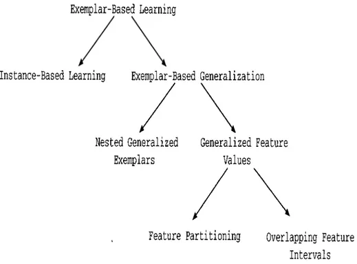
Figure 2.1. CIa,ssification of exemplar-based lecirning models.

2.1

Exemplar-Based Learning

Exemplar-based learning was originally proposed as a model of human learning by Medin and Schaffer [41]. In the simplest form of exemplar-based learning, every example is stored in memory verbatim, with no change of representation. An example is defined as a vector of feature values along with a label which represents the category (class) of the example.

Knowledge representation of exemplar-based models can be miiintained as representative instances [2, 5], hyperrectangles [58, 59], or generalized vcilues [27, 28, 67]. Unlike explanation-based generalization (EBG) [18,

45

], little or no domain specific knowledge is required in exemplar-based learning.

Pdgure

2.1

presents a hierarchical classification of exemplar-based learning models. Instance-based learning (IBL) and exemplar-based generalization cire two types of exemplar-based learning. For example, instance-based learning methods [5] retain examples in memory cis points, and never chcinges them.

On the other hand, exemplar-based generalization methods make certain gen­ eralizations on the training instances. One category of the exemplar-based gen- ei'cilization is the nested-generalized exemplars (NGE) model [58]. This model changes the i^oint storage model of the instance-bcised learning and retains examples in the memory as axis-parallel hyperrectangles. Generalized Fea­ ture Values learning models can be classified as exemplar-based genei'cdization, such as NGE. The examples of GFV learning models are the Classification by Feature Partitioning (CFP), and the Classification by Overlapping Feature In­ tervals (COFI). In the CFP algorithm, examples are stored as disjoint intervals on each feature dimension. In the COFI algorithm, concept descriptions are represented in the form of overlapping feature intervals. In this thesis, we will study several batch learning methods whose knowledge representation is in the form of disjoint feature intervals that can be also categorized as GFV method. In the following sections, we will describe IBL, NGE, and GFV methods briefly. GFV methods that use feature projections for knowledge representation will be discussed in detail in Chapter 3 since this knowledge representation motivated us to develop this thesis.

2.1.1

Instance-Based Learning (IBL)

Instance-based learning algorithms represent concept descriptions as a set of stored instances, called exemplars, and with some information concerning their past performances during classification [5,

8

]. These algorithms extend the clas­ sical nearest neighbor algorithm, which has hirge storage requirements [16, 17]. All examples are represented as points on the ?r-dimensional Euclidean space, where n is the number of features. The concept descriptions can change after each training instance is processed. IBL algorithms do not construct exten- sional concept descriptions. Instead, concept descriptions are determined by how the IBL algorithm’s selected similarity and classification functions use the current set of saved instances. There are three components in the framework which describe all IBL algorithms as defined by Aha and Kibler [5]:

1

. The similarity function computes the similarity between two instances (similarities are real-valued).

2

. The classification function receives the output of the similarity function and the classification performance records of the instances in the concept description, and yields a classification for instances.

3. The concept description updater maintains records on classification per­ formance and decides which instance are to be included in the concept description.

These similarity and classification functions determine how the set of in­ stances in the concept description are used for prediction. So, IBL concept descriptions contain not only a set of instances, but also these two functions.

Several IBL algorithms have been developed; IB l, IB

2

, IB3, IB4 and IB5 [3, 5]. IBl is the simplest one and it uses the similarity function computed as

similarity[x^ y)

(

2

.

1

)

\xf — yf\ if / is linear

0

if f is symbolic and x j = y j (

2

.

2

)

1

if f is symbolic <ind x j ^ i j f

where x and y are the instances.

IBl is identical to the nearest neighbor algorithm except that it processes training instances incrementally and simply ignores instances with missing fea­ ture value(s). Since IB l stores all the training instances, its storage requirement is quite large. IB2 is an extension of IB l, it saves only misclassified instances reducing storage requirement. On the other hand, its classification accuracy decreases in the presence of noisy instances. IB3 aims to cope with noisy in­ stances. IB3 employs a significance test to determine which instances cire good classifiers and which ones are believed to be noisy. Once an example is deter­ mined to be noisy, it is removed from the description set. IB2 and IB3 are also incremental algorithms. IB l, IB2, and IB3 algorithms assume that all features have equal relevance for describing concepts.

Extensions of these three algorithms [

1

, 3] are developed to remove some limitations which occur because of certain assumptions. For example, concepts are often assumed to

• be defined with respect to the same set of relevant features, • be disjoint in instance space, and

• have uniform instance distributions.

To study the effect of relevances of features in IBL algorithms, IB

4

has been proposed by Aha [3]. In this study, feature weights are learned being dependent on concepts; a feature may be highly relevant to one concept and completely irrelevant to another. So, IB4 has been developed as an extension of IB3 that learns a separate set of feature weights for each concept. Weights are adjusted using a simple feedback algorithm to reflect the relative relevances of the features to describe instances. These weights are then used in IB

4

’s similarity function which is a Euclidean weighted-distance measure of the sim­ ilarity of two instances. Multiple sets of weights are used because similarity is concept-dependent, the similarity of two instcinces varies depending on the target concept. IB4 decreases the effect of irrelevant features on classification decisions. Therefore, it is quite successful in the presence of irrelevant features.

The problem of novelty is defined as the problem of learning when novel features are used to help describe instances. IB4, similar to its predecessors, assumes that all the features used to describe training instances are known before training begins. However, in several learning tasks, the set of describing features is not known beforehand. IB5 [3], is an extension of IB4 that tolerates the introduction of novel features during training. To simulate this capability during training, IB4 simply assumes that the values for the (as yet) unused feature are missing. During training, IB4 fixes the expected relevance of the feature for classifying instances. IBS instead updates the weight of a feature only when its value is known for both of the instances involved in a classification cittempt. IBS can therefore learn the relevance of novel features more quickly than IB4.

Also noise-tolerant versions of instance-based algorithms have been devel­ oped by Aha and Kibler [4]. These learning algorithms are based on a form of significance testing, that identifies and eliminates noisy concept descriptions.

2.1.2

Nested-Generalized Exemplars (N G E )

Nested-generalized exemplar (NGE) theory is a variation of exemplar-based learning [58]. In NGE, an exemplar is a single training example, and a general­ ized exemplar is an axis-parallel hyperrectangle that may cover several training examiDles. These hyperrectangles may overlap or nest. Hyperrectangles are grown during training in an incremental manner.

Salzberg implements NGE in a program called EACH (Exemplar-Aided Constructor of Hyperrectangles) [59]. In EACH, the learner compares new examples to those it has seen before and finds the most similar generalized exemplar in memory.

NGE theory makes several significant modifications to the exemplar-bcised model. It retains the notion that examples should be stored verbatim in mem­ ory, but once it stores them, it allows examples to be generalized. In NGE theory, generalizations take the form of hyperrectangles in ?r-dimensional Eu- clidecin space, where the space is defined by the feature values mecisured for each example. The hyperrectangles may be nested one inside another to arbi­ trary depth, and inner rectangles serve as exceptions to surrounding rectangles [58]. Each new training example is first classified according to the existing set of classified hyperrectangles by computing the distance from the example to each hyperrectangle. If the training example falls into the necirest hyper­ rectangle, then the nearest hyperrectangle is extended to include the training example. Otherwise, the second nearest hyperrectangle is tried. This is called as second match heuristic. If the training example falls into neither the first nor the second nearest hyperrectangle, then it is stored as a new (trivial) hy­ perrectangle.

A new example will be classified according to the class of the necirest hy­ perrectangle. Distances are computed as follows: If an example does not fall

into any existing hyperrectangle, a weighted Euclidean distance is computed. If the example falls into a hyperrectangle, its distance to that hyperrectangle is zero. If there are several hyperrectangles having equal distances, the smallest of these is chosen. The EACH algorithm computes the distance between E and H, where E is a, new data point and H is the hyperrectangle, by measuring the Euclidean distance between these two objects as follows;

where De,h = wh d ( E , H J )

\

^ 2^ (“>/---— rmax f — min f h j j > H f^ u p p e r H J flower E f E f <C Hfjower 0 otherwise (2.3) (2.4)

where wh is the weight of the exemplar H, Wf is the weight of the feature / ,

E f is the value of the /t h feature on example E , Hj^upper or H},lower are the upper end of the range and lower end, respectively, on /t h feature on exemplar / / , m axf and mirif are the minimum and maximum values of that feature, and n is the number of features recognizable on E.

The EACH algorithm finds the distance from E to the nearest face of H. There can be several alternatives to this, such as using the center of H. If the hyperrectangle H is a point hyperrectangle, representing an individiuil example, then the upper and lower values becomes equal.

If a training instance E and generalized exemplar H are of the same class, that is, a correct prediction has been made, the exemplar is generalized to in­ clude the new instance if it is not already contained in the exemplar. However, if the closest hyperrectangle has a different class then the algorithm modifies the weights of features so that the weights of the features that caused the wrong prediction is decreased.

The original NGE was designed for continues features only. Symbolic fea­ tures require a modification of the distance and area computations for NGE.

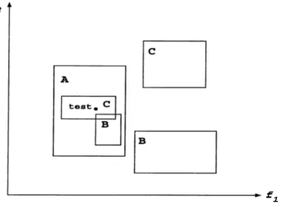
Figure

2

.

2

. An example concept description of the EACH algorithm in a do­ main with two features.

In Figure 2.2, an example concept description of EACH algorithm is pre­ sented for two features / i and /

2

. Here, there are three classes. A, B and C, and their descriptions are rectangles (exemplcirs) as shown in Eigure

2

.

2

. It is seen that rectangle A contains two rectangles, B and C', in its region. Therefore, B and C are exceptions in the rectangle A. The NGE model allows exceptions to be stored quite easily inside hyperrectangles, and exceptions can be nested any number of levels. The test instance, that is marked as test in Figure 2.2, falls into the rectangle C, since it has smaller, so the prediction will be the class value C for this test instance.

2.1.3

Generalized Feature Values

The previously presented techniques categorized as generalized feature values under exemplar-based generalization are the CFP [27, 28, 65], COFI [67], and A:-NNFP [7] algorithms. Briefly, the CFP and COFI algorithms are incremental algorithms based on feature partitioning and overlapping feature intervals, re­ spectively. They use feature projections as the basis of learning. Classification of unseen instances are based on voting among the individually predictions of features. The discussion of the CFP and COFI algorithms are presented in Chapter 3 in more detail (Section 3.1 and

3

.

2

).

2.2

Decision Trees

Decision trees are one of the most well known and widely used approaches for learning from examples. This method was developed initially by Hunt, Marin and Stone [31], and later modified by Quinlan [49, 50]. Quinlan’s ID3 [52] and C4.5 [55] are the most popular algorithms in decision tree induction. Initially, ID3 algorithm has applied to deterministic domains such as chess and games [49, 50]. Later, ID3 algorithm has extended to cope with noisy and uncertain instances rather than being deterministic [52].

Decision tree algorithms represents concept descriptions in the form of tree structure. Decision tree algorithms begin with a set of instances and create a tree data structure that can be used to classify new instances. Each instance is described by a set of feature values, which can have either continuous or symbolic (nominal) values, with the corresponding classification. Each internal node of a decision tree contains a test which indicates which branch to follow from that node. The leaf nodes contain class labels instead of tests. A new test instance is classified by using the class label stored at the leaf node.

Decision tree methods use divide and conquer approcvch. Each internal node must contain a test thcit will partition the training instances. The most important decision criteria in decision tree induction is how to decide the best test. ID3, and its successor C4.5 use information-theoretic metrics to evaluate the goodness of a test; in particular they choose the test that extracts the maximum amount of information from a set of instances, given the constraint that only one feature will be tested.

The recursive partitioning method of constructing decision trees continues to subdivide the set of training instances until each subset in the partition con­ tains instances of a single class, or until no tests offer any further improvement. The result is often a very complex tree that “overfits the data” by inferring more structure than is justified by the training instances. A decision tree is not usually simplified by deleting the whole subtree in favor of a leaf. Instead, the idea is to remove parts of the tree that do not contribute to classifica­ tion accuracy on unseen instances, producing something less complex and thus

more comprehensible. This process is known as the pruning. There are basi­ cally two ways in which the recursive partitioning method can be modified to produce simpler trees: deciding not to divide a set of training instances any further, or removing retrospectively some of the structure built up by recursive partitioning [55].

The former approach, sometimes called stopping or prepruning., has the advantage that time is not wasted in assembling structures that are not used in the final simplified tree. The typical cipproach is to look at the best way of splitting a subset and to assess the split from the point of view of statistical significance, information gain, error reduction. If this assessment falls below some threshold then the division is rejected.

Later, a simple decision tree approach, called IR system, is proposed by Holte [30]. It is based on the rules that classify an object on the basis of a single feature that is, they are 1-level decision trees, called 1-rules [3'

The input of the IR algorithm is a set of training instances. The output is concept descriptions in the form of 1-rule. The IR system can be treated as a special case of generalized feature values methods. These methods consider all features information whereas the IR system uses only one feature. IR tries to partition feature values into several disjoint feature intervals. Since each feature is considered separately in IR system, missing feature values can be simply ignored instead of ignoring the instance containing missing value. The FIL algorithms presented in this thesis also partition feature dimensions into disjoint intervals. However, the FIL algorithms make final predictions based on majority voting on individual classifications of all features rather than one feature as in IR system. During the training phase of the IR system, disjoint feature intervals are constructed on each feature dimension. Then, one of the concept descriptions on a feature is chosen as final concept descriptions, 1-rules, by selecting the one that makes the smallest error on the training dataset.

Holte used sixteen datasets to compare IR and C4 [52], and fourteen of the datasets were selected from the collection of UCI-Repository [47] [30]. The main result of comparing IR and C4 was an insight into the tradeoff between

simplicity and accuracy. IR rules are only a little less accurate (about 3 per­ centage points) than C4’s pruned decision trees on almost all of the datasets. Decision trees formed by C4 are considerably larger in size than 1-rules. Holte shows that simple rules such as IR are as accurate as more complex rules such as C4.

Another decision tree algorithm is T2 (decision trees of at most 2-levels) [12]. Its computation time is almost linear in the size of training set. The T2 algorithm is evaluated on 15 common reid-world dataset. It is shown that the most of these datasets, T2 provides simple decision trees with little or no loss in accuracy compared to C4.5.

2.3

Statistical Concept Learning

Statistical concept learning has been extensively studied for induction problems [21, 25, 69]. The main goal is to determine the classification of a given instcuice based on parametric or nonparametric techniques. The decision-making pro­ cesses of humans are somewhat related to the recognition of patterns. For example the next move in chess game is based upon the present pattern on the board, and buying or selling stocks is decided by a complex pattern of information [25]. The goal of the pattern recognition is to clarify these com ­ plicated mechanisms of decision-making processes and to automate these func­ tions using computers. Several pattern recognition methods, either parametric or nonparametric, have been presented in the literature [20, 21, 25, 69].

Bayesian classifier originating from work in pattern recognition is a proba­ bilistic approach to inductive learning. This method estimates the (posterior) probability that an instance belongs to a class, given the observed feature val­ ues for the instance. The classification is determined by the highest estimated posterior probability [21, 25]. Bayesian chissifiers assume that features are sta­ tistically dependent. On the other hand. Naive Bayesian classifier is one of the most common parametric classifiers assuming independence of features.

When no parametric structure can be assumed for the density functions, nonparametric techniques, for instance nearest neighbor method, must be used

for classifications [21, 25]. The nearest neighbor method is one of the simplest methods conceptually, and is commonly cited as a basis of comparison with other methods. It is often used in case-based reasoning [62].

This section is devoted to statistical concept learning methods because they have similarities to the FIL algorithms developed in this thesis F’irst, Bayes Decision Theory and Naive Bayesian Classifiers will be explained. Then, nearest neighbor methods with some variants will be discussed. Finally, a new version of k nearest neighbor algorithm, A;-NNFP, based on feature projections will be briefly mentioned, and discussed in detail in Chapter 3 by comparing k nearest nearest neighbor techniques. In Chapter 5, the FIL algorithms will be compared with these statistical methods.

2.3.1

Bayes Decision Theory - Naive Bayesian Classi­

fier (N B C )

The goal of the Bayesian classification is to determine the a posteriori proba­ bilities P { C j \ x ) where C j is the class and x is the instance to be classified. An instance x = < x i,X2·, ■■■Xn > is a vector of feature values where n is the num­ ber of features. The a priori probability P { C j ) and the conditional densities

P { x \ C j ) allows the use of Bayes rule to compute P ( C ' , [ x ) .

Let D = {C l, C

2

, .·, Ck} be the finite set of k states of nature. Here each C j

corresponds to a class in our terminology. Let the feature vector x be a vector­ valued random variable, and let p { x \ C j ) be the state-conditional probcibility density function for x , that is, the probability density function for x conditioned on C j being the state of nature. Finally, let P { C j ) be the a priori probability that nature is in the state C j . That is, P { C j ) is the proportion of all instances of class j in the training set. Then the a posteriori probability P { C j \ x ) can be

computed from p { x \ C j ) by Bayes rule [21]:

p(x|C,)C (C i)

P(Cj\x.)

pM

(2.5)

pW = Y ,p {^ \ C j)P (C j).

i=i

(2.6)

Let A = { «i,Q

!25

be the finite set of a possible actions. Let X {ai,C j)

be the loss incurred for taking action ai when the state of nature is C j . Since

P{Cj\'x.) is the probability that the true state of nature is C j , the expected loss

cissociated with taking action ai is

Ricxil^) = J2\{ai\Cj)P{CM)· (2.7)

i=l

In decision theoretic terminology, an expected loss is called risk, and R(cxi |x) is known as the conditional risk. Whenever we encounter a particular observa­ tion X , we can minimize our expected loss by selecting the action that minimizes

the conditional risk. Now, the problem is to find a Bayes decision rule against

P { C j ) that minimizes the overall risk. A decision rule is a function a (x ) that tells us which action to take for every ¡possible observation. That is, for every

X , the decision function o;(x) assumes one of the a values cri, «2, ··) «a· The

overall risk R is the expected loss associated with a given decision rule. To minimize the overall risk, we compute the conditional risk for i = l ,. ., a and select the action ai for which i?(ai|x) is minimum. The resulting minimum overall risk is called the Bayes risk and is the best performance that can be achieved.

H(a.|x) = X:A (ai|Q )P(Cj|x)

i=l

(

2

.

8

)

The probability of error is the key parameter in pattern recognition. There are many ways to estimate error for Bayesian classifiers. One of them is mini­ mizing it. For example, if action ai is taken and the true state of nature is C j ,

then decision is correct if z = j , and in error ii i ^ j . A loss function lor this case, called zer'o-one loss function is:

a 0 if z = j

1 if z 7^ j (2.9)

The conditional risk becomes

/2(0!.·| x ) ^ ^ P ( C j \ x ) (

2

.

10

)

R( ai \ x) = 1 - P { Ci \ x ) (

2

.

11

)

Note that P { C i \ x ) is the conditional probability that action ai is correct. To minimize the average probability of error, one should maximize the a posteriori probability P (6j |x). For minimum error rate;

Decide Ci if P { C i \ x ) > P { C j \ x ) for all j z.

In summary, a Bayesian classifier classifies a new instance by cipplying Bayes’ rule to determine the probability of each class given the instance.

P ( C M ) =

p ( x \ C j ) P ( C j )

E . p ( x | C i ) P ( C . )

(

2

.

12

)

The denominator sums over all classes and where P { x \ C j ) is the probability

of the instance x given the class C j . After calculating these quantities for each

class, the algorithm assigns the instance to the class with the highest proba­ bility. In order to make this expression operational, one must specify how to compute P { x \ C j ) . The Naive Bayesian Classifier (NBC) assumes independence of features within each class, allowing the following equality

n ^ | c ,) = n /=1

(2.13)

An analysis of Bayesian classifier has been presented [36]. Also a method, called Selective Bayesian Classifier, has been proposed [37] to overcome the

limitation of the Bayesian classifier for sensitivity to correlated features. Since NBC considers each feature independently, this will form a basis lor comparison with the FIL algorithms. The experimental results of these comparisons will be presented in Chapter 5.

2.3.2

Nearest Neighbor Classifiers (N N )

One of the most common classification techniques is the nearest neighbor (NN) algorithm. In the literature, nearest neighbor algorithms for learning froixi examples have been studied extensively [17, 21]. Aha et al. have demonstrated that instance-based learning and nearest neighbor methods often work as well as other sophisticated rnachjne learning techniques [5].

The NN classification algorithm is based on the assumption that examples which are closer in the instance space are of the same class. An example is represented as a vector of feature values plus class label. That is, unclassified ones should belong to the same class as their nearest neighbor in the ti'ciining dataset. After all the training set is stored in memory, a new example is classi­ fied as of the class of the nearest neighbor among all stored training instances. Although several distance metrics have been proposed for NN algorithms [60], the most common metric is the Euclidean distance metric. Instances are rep­ resented as a vector of feature values plus class label. The Euclidean distance between two instances x = < x i,X2, ...,Xn,Cx > and y —< y i,y₂, ...yn,Cy > on

an n dimensional space is computed as:

dist{x, y) = d i f f { f , x , y ) = y E % , d i f f { f , x , , j Y (2.14) \^f ~ Vf\ if / is linear 0 if f is nominal and Xf = y/ (2.15) 1 if f is nominal and x ¡ ^ yj

Here d i f f { f , x, y) denotes the difference between the values of instances x, and y on feature / . Note that this metric requires the normalization of all feature values into a same range.

Although several techniques have been developed for handling unknown (missing) feature values [54, 55], the most common approach is to set them to the mean value of the values on corresponding feature.

Stanfill and Waltz introduced the Value Difference Metric (VDM ) to define the similarity for symbolic-valued (nominal) features and empirically demon­ strated its benehts [62]. The VDM computes a distance for each pair of the different values a symbolic feature can assume. It essentially compares the relative frequencies of each pair of symbolic values across all classes. Two fea­ ture values have a small distance if their relative frequencies are approximately equal for all output classes. Cost and Salzberg present a nearest neighbor algorithm that uses a modification of VDM, called MVDM (Modified Value Difference Metric) [15]. The main difference between MVDM and VDM is that their method’s feature value differences are symmetric. This is not the case for VDM. A comparison of MVDM and Bayesian classifier is presented in [56].

A generalization of the nearest neighbor algorithm, A:-NN, classifies a new instance by a majority voting among its /: (> 1) nearest neighbors using some distance metrics in order to prevent the intrusive effect of noisy training in­ stances. This algorithm can be quite effective when the features of the domain are equally important. However, it can be less effective when many of the features are misleading or irrelevant to classification. Kelly and Davis intro­ duced WKNN, the weighted ¿-NN algorithm, and GA-W KNN, a genetic algo­ rithm that learns feature weights for WKNN algorithm [33]. Assigning variable weights to the features of the instances before applying the k-NN algorithm distorts the feature space, modifying the importcince of each feature to reflect its relevance to classification. In this way, similarity with respect to impor­ tant features becomes more critical than similarity with respect to irrelevant features. The study for weighting features in /?-NN algorithm has shown that for the best performance the votes of the k nearest neighbors of a test exam­ ple should be weighted in inverse proportion to their distances from the test example [70].

An experimental comparison of the NN and NGE {Nested Generalized Ex­ emplars, a Nearest-Hyperrectangle algorithm) has been presented by Wettschereck

and Dietterich [71]. NGE and several extensions of it are found to give pre­ dictions that are substantially inferior to those given by A;-NN in a variety of domains. An average-case analysis of fc-NN classifiers for Boolean threshold functions on domains with noise-free Boolean features and a uniform instance distance distribution is given by Okamoto and Siitoh [48]. They observed that the performance of the A;-NN classifier improves as k increases, then reaches a maximum before starting to deteriorate, and the optimum value of k increases gradually as the number of training instances increases.

2.3.3

N N Classifier on Feature Projections (N N F P )

Another statistical approach is a new version of the A;-NN classification al­ gorithm proposed in this thesis, which uses feature projections of training instances for classification knowledge [7]. The classification of an unseen in­ stance is based on a majority voting on individual classifications made by the projections of the training set on each feature. We have applied the ^;-nearest neighbor algorithm to determine the classifications made on individual feature projections. We called the resulting algorithm A:-NNFP, for A:-Nearest Neighbor on Feature Projections. The classification knowledge is represented in the form of projections of the training data on each feature dimension. This allows the classification of a new instance to be made much faster than A;-NN algorithm. The voting mechanism reduces the intrusive effect of possible irrelevant fea­ tures in classification. The A:-NNFP algorithm is discussed in detail in Section 3.3.