Decoherence in open quantum systems : a realistic approach

(1)

DECOHERENCE IN OPEN QUANTUM

SYSTEMS: A REALISTIC APPROACH

A THESIS

SUBMITTED TO THE DEPARTMENT OF PHYSICS AND THE INSTITUTE OF GNGINEEIUNG AND SCIENCE

OF BILKENT UNIVERSITY

IN PARTIAL FULFILLMEXT OF THE REQUIREI'vfE~TS FOR THE DEGREE OF

DOCTOR OF PHILOSOPHY

By

Kerim Savran

J

anuary 2006

(2)

T certi~y that T have read this thesis and that in my opinion it is fully adequate, in scopc and in quality, as a disscrtation for the dcgrce of doctor of philosophy.

i\s,;oc. Prof_ Tuğrul Hakioğlu (Supervisor)

I c:ertify that I have read this thesis and that in my opinion it is fully adequate, in scopc and in quality, as a disscrtation for the dcgrce of doctor of philosoplıy.

Prof_ Dr. Alexander Shıımovsky

T cert.ify that T have read this thesis and that in my opinion it is fully adequate, in scope and in quality, as a dissertation for the degree of doctor of philosophy.

(3)

T certi~y that T have read this thesis and that in my opinion it is fully adequate, in scopc and in quality, as a disscrtation for the dcgrce of doctor of philosophy.

Prof Dr. l'vldııııd Toıııak

I c:ertify that I have read this thesis and that in my opinion it is fully adequate, in scopc and in quality, as a disscrtation for the dcgrce of doctor of philosoplıy.

Assist. Prof Oğuz Gülseren

A pproved for the Institute of Engineering and Science:

Prof. :VIelıınet Baray,

(4)

Abstract

DECOHERENCE IN OPEN QUANTUM SYSTEMS: A

REALISTIC APPROACH

Kerim Savran

PhD in Phvsics

"

Supervisor: Assoc. Prof.

Tuğrul Hakioğlu

J

anuaı-y

2006

Dccolıercnce nıcdıanisnıs of opcıı quantum systems ın intcractioıı with an cnvironırıcntal bath is invcstigat.cd using the master equation formalism. VViddy used two-level approximation is questioned.

It has been shown that decoherence has different behavior in short and long time regimes. In short times, decoherence mechanisms, relaxahon, dephasing and leakage shmv a Gaussian-like behavior, whereas in the long time regime, they have exponential-like bdıavior as predicted by the Markov approxinıation. The non-ncgligiblc cffccts of the non-resonant transitionsin the short time regime is observed tu be more destructive in tenm·ı of decoherence, than the long time resona.nt transitions. ~/Iultilevel effects are also investigatecl in order to question the validity of the two-level approximation. It has been observed that the higher levels above the qubit subspace have signifıcant eliec-Ls in decoherence ratcs. Tlıerefore, the assumptions of the two-levcl approxiınation are proved to be irrclcvant •vith the validity of the two-lcvcl approximation. The rcliahility analysis of the Born-Oppenheimer approximation, which is the only approxiınation used, is also been explainecL

(5)

Finally, the outcome of the driving fields, >vhich are tools for the manıp ulation of quantum systems, for a multilevel opcıı quantıım system has been

dcınonstratcd. IL has bccn slıuwn that. Rabi oscillations cannot be obscrvcd in a

mıılti-lcvclcd system as snıoothly as in a two-lcvclcd syst.em.

Keywords: Decoherence, Master Equalion Formalism, Non-resonant Tran-sitions, ı'vlultilcvcl SysLems, Twc}-lcvcl Approximation, I3orn-Oppenheimer Approxiınation, Rabi Oscillations.

(6)

••

O

zet

.

AÇIK KUVANTUM SISTEMLERDE UYUMSUZLUK:

_{. .}

GERÇEKÇI BIR

YAKLAŞlM

Kerim Savran

Fizik Doktora

Te~

Yöneticisi: Assoc.

Prof.

Tuğrul Hakioğlu

Ocak 2006

Çevresel bir rezervuar ilc etkileşimele olan açık kuvantunı sistemlerindeki uyumsuzluk mekanizmalan ana denklem formalizmi kullanılarak incelendi. Yaygın olarak kullanılan iki-seviye yaklaşıldığı sorgulandı.

U_yumsuzluğun kısa ve uzun zaman bölgelerinde farklı davranışlar gösterdiği gösterildi. Kısa zamanlarda uyumsuzluk mekanizmaları, dunılma, eqevre k..-ı,ybı ve

sızıntı, Gaussal-benzeri bir davranış gösterirken, uzun zamanlarda 1/Iarkov yakla.jıklığının öngördüğü sekilde üstcl davranış gösteriyorlar. Kısa zamanlardaki ihmal cdilcmcyccck rezonant olmayan gcçi~lcrin, uyumsuzluk koııusıında uzun zamanlardaki rezarıant geçişlerden daha yıkıcı oldugu gözleınlendi. 1 ki seviye yakla.~ıklığırıın geçerliliğini sorgulamak için çok-seviye etkileri de incelendi. Kubit alt-uzayının üstündeki enerji seviyelerinin uyumsuzluk zamanları üzerinde önemli etkileri olduğu gözlemlendi. Dolayısıyla, iki-seviye yakla.şıklığı için öngörülen varsayıınların, yakla§ıklığın geçerliliği ilc ilgili olmadığı gösterildi. Kullanılan tck yakla§ıklık olan Born-Oppenheimer yaklaşıklığının da güvenilirlik analizi yapıldı. Son olarak, kuvantum sistemlerin ınanipıılasyonıında kullanılan sürücü alan-ların çok seviyeli açık kuvantum sistemlerindeki sonuçları gösterildi. Çok

(7)

seviyeli sistemlerde Rabi salınımlarının iki seviyeli sistemlerdeki kadar kolay elde

edilemeyeceği gözlendi.

Anahtar

sözcükler: Kuva.nLum Uyumsuzluk, Ana. Denklem Forma.lizmi~ Rezo-nant Olmayan Geçi§ler, Çok Seviyeli Sistemler, İki Seviye Yaklcı§ıklığı, Born-Oppenheimer Yakla§ıklığı, Ra.bi Salınımla.rı.

(8)

Acknow ledgement

I would like to express my deepest gratitude to Assoc. Prof. Tuğrul Hakioğlu for his supervision during research, guidance and understanding throughout this thesis.

I like to thank to all my friends in physics department, as they kept my morale up all the time. I also like to express my thanks to Haldun Sevinçli for the discussions on the last chapter.

I am also grateful for the improvements on my text made by Assoc. Prof. Ulrike Salzner and Çağrı Öztürk.

Last but not the least, I would like to thank my family for their never ending support.

(9)

.

lV Vl vii i ıx X ll XIX ı 4 5 5 6 7 8 10 10 12 13 10

(10)

2.2.S A general application 2. 3 l\:Iodels . . . .

2.:3.1 Spin-boson model . 2.:3.2 Central spin model 2.3.:3 Rlocl1-Redfield model .

2.3.4 Lindblad formalisın . .

3 Superconducting systems and the Josephson effect

3.1 .Josephson effect . . . . 3.1.1 The R.CS.J model . . . .

3.1.2 .Josephson eiTecL in the prcscnec of magnetic 11ux .

3.2 SQUID dcviccs .

3.2.1 dc-SQUID

:3.2.2 rf-SQUID

:3.2.3 SQUTD-El\if field model.

4 Noise and decoherence of the system

4.1 Decolıerence in SQ UID-E.:vi fieldmodel 4.2 Spectral dependencies 4.2.1 4.2.2 4.2.3 4.2.4 4.2.5 4.2.() Temperature . . O hmic dependencies Cut-off frequency Spectral center . Spectral widtlı . Spectral amplit.ude

5 Effects of Noise Parameters in Decoherence .5.1 Decolıerence rates at slıort and long times .5.2 1\·'lultilevel efl'ects 5.2.1 Leakage . 5.3 NonresonanL e1Iec:Ls 5.:3.1 Short-tinıe bclıavior . X 18 22 22 24 25 27 29 29 30 3~1 35 36 37 :38

45

46 54 55 60

60

62 64 65 68 70 73 75

76

77

(11)

5.3.2 Long-time behavior . . . . 5.4 Limit.alions of the I3onı-Oppenheinıer approximation 6 Driving fields in the realistic system-environment model

6.1 Rabi oscillations . . . .

6.2

6.1.1 The dfect of higlıer lcvds 6.1.2 The cffcct of the cnvironmcnt.

6.1.3 Expected outcorne of realistic Rabi oscillations . NOT gate simulation

7 Conclusions

A The analysis of the compensating term B Proof of the reality and positivity of A (G)

C N um erical code Xl 80 82

87

88 89 91 92 95

99

101 105 107

(12)

List of Figures

3. ı The effective circuit used in the RCSJ model. 3. 2 The tilted-washboard potential for I/ Ico

=

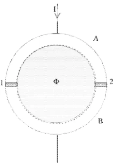
0.1.

3. 3 A circular ring with two Josephson junctions. The dotted lines 3ı 32

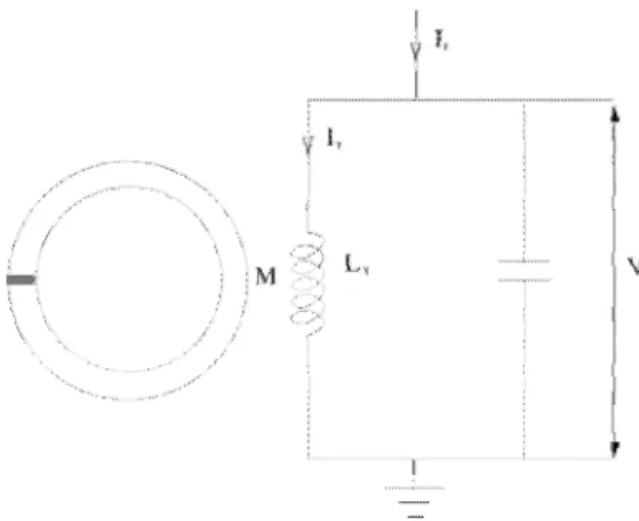
indicate the cantour for the integration. . . 34 3. 4 A rf-SQUID coupled to a rf circuit with mutual inductance

coupling M. . . 38 3. 5 A rf-SQUID coupled to an electromagnetic field with mutual

inductance coupling M. There is also an external fiux <I>x effecting the SQUID ring.

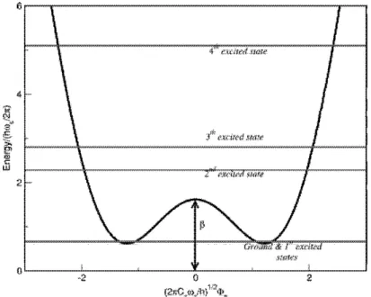
3. 6 The potential and low lying energy eigenvalues, for a specific single degenerate case. Here the parameters are (3 "':' 1.6ı6 and 1 "':' 1. 753. The axes are normalized and dimensionless.

3. 7 The potential and low lying energy eigenvalues, for a specific double degenerate case. Here the parameters are (3 "':' O. 772 and

39

43

1 "':' 2.ı87. The axes are normalized and dimensionless. . . 44 4. ı The dipole matrix elements defining the transitions from ground

and first excited state for a specific single degenerate case. Here the parameters are (3 "':' 1.6ı6 and 1 "':' 1. 753. Here, the potential wells are symmetric with !f!x = 0.5 . . . 47

4. 2 The dipole matrix elements defining the transitions from ground and first excited state for a specific single degenerate case. Here the parameters are (3 "':' 1.6ı6 and 1 "':' 1. 753. Here, the potential wells are asymmetric with !f!x = 0.6 . . . 48

(13)

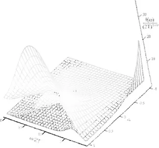
4. 3 The variation of the spectral functioıı I (w) versus w and v for

-1 .::=; ı; .::=; 1 and pa.rametrized as A/T = 10, SO, 100 from the inncrmost to the outcrmost sıırfaccs respectively. . . . 51 4. 4 The variation of the spectral hınction I (w) versus w for Lorcntzian

spectrum. Tn (a), E= 0.5 and w0 = 4 are fixecl parameters whereas

A changes. Tn (b), E = 0 .. 5 and A = 3 are fixed pammeters and

w0 changes. In (c), w0

=

4 and A

=

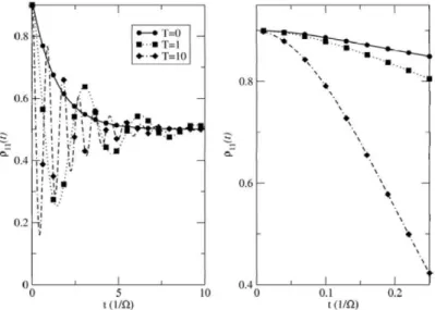
3 are fixecl pa.ra.meters and E changes. . . . . .

4. 5 The rclaxation curvcs for a degencratc two lcvd system, that is in intcraction with a power-law type spectrum wit.h A = 10 and

v = -1 for various tempemtures. On the left; we have a broader time range \vhere time is nonnalizeel with an energy scale

n,

and

52

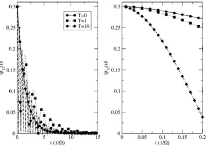
on the right we obsen'e closely the short time range. . . 5ô 4. 6 The dephasing curves for a degenerate tvm level system, that is

in intcraction with a power-law type spectrum wit.h A = 10 and

11 = -1 for various tempera.tures. On the left; wc have a broadcr time range where time is nonnalizeel with harmonic frequency, and on the right \\'e observe closel.Y the short time range. . .

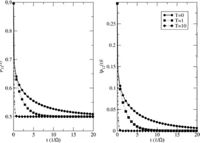
4. 7 The relaxation and dephasing curves for a. degenerate two level system, that is in intera.ction -.,vith a power-law type spectrıım with

57

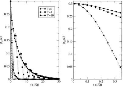
A = 10 and 11 = O for various temperatııres. . . . 58 4. 8 The rdaxation curves for a degcnerat.e two lcvd system, that. is in

interaction with a Lorentzian type spectrunı with A = 3, E = 3

and w₀= 5 for various temperatures. On the left side is the overall behavior 'ivhere short time range is magnified on the right hand side. 58 4. 9 The dephasing cun•es for a. degenerate tvm level system; that is in

intcraction wit.h a LorcnLz;ian type spectrum witlı A =

:i,

f = 3

and w₀= 5 for various teınperatures. On the lcft sidc is the overall behavior where short time range is ınagnified on the right hand side. 59

(14)

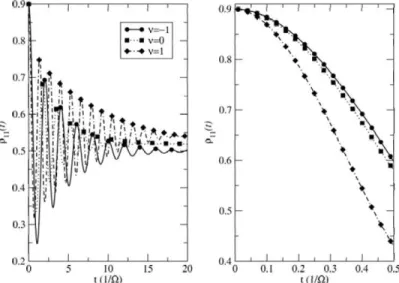
4. 10 The relaxation cunres for a degenerate two level system, that is in interaction with a. power-law type spectrıım >vith A = 1, T = O

for varioııs IJ values. On the lcft side is the overall bdıavior where

short time range is magnified on the right. lıand sidc. . . 61 4. 11 The dephasing curves for a degenerate two level system; that is in

interaction with a power-law type spectrunı with /\. = 1, T = -for ·various v values. On the left side is the overall behavior where

short time range is magnified on the right hand side.

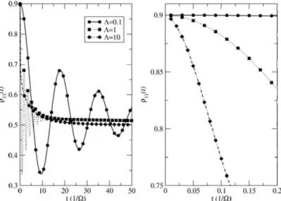
4. 12Tlıe rclaxation curves for a dcgcncrate two lcvd system, that is in internetion witlı a pmver-law type spectrum \vith lJ

=

O, T

=

O for various ;\ values. On the left side is the overall behavior "vhere short time range is magnified on the right hand side.

4. 1:3 The dephasing curves for a degenerate hvo level system, that is in interaction with a pmver-law type spectrıım with 11 =O, T =O for

various A valnes. On the ldı. side is the overall bchavior where 61

62

short time range is magnified on the right. lıand sidc. . . 63

4. 14 The relaxation curves for a degenerate two level system, that is in interaction with a Lorentzian type spectnurı with A = 3 and E = 3 for various w0 values. On the left side is the uverall behavior where

short time range is magnified on the right hand side. . . 64

4. 15 The dephasing curves for a degcncratc t.vm lcvd system; that is in intcmdinn with a Lorcntzian type spectrum with A_ = 3 and ıc = 3 for various w₀= 5 values. On the left side is the overall behavior where short time range is magnified on the right hand sicle. . . 65 4. Hi The relaxation curves for a clegenerate two level system, that is

in interaction with a. LorenL;,-;ian type spectnım with A_ = ~) and

w₀= 5 for varioııs f valnes. On the ldı. sidc is the overall bclıavior where short time range is ımı.gnified on the right lıand sidc. . . 65

(15)

4. 17The dephasing curves for a degenerate t\vo level system, that is in interaction with a LorenL;,-;ian type spectrum 'Nith A = ~) and

w₀= 5 for varioııs f valucs. On the ldt. sidc is the overall hchavior

·where short time rangc is ınagnified on the right lıand sidc. . . 66 4. 18The relaxation curves for a degenerate two level system, that is

in interaction with a Lorentzian type spectrurn witlı E = 3 and w0 = 5 for various spectral anıplitucles. On the left side is the

overall behavior where short time range is magnifıed on the right hand sidc. . . 67

4. 19The dephasing curvcs for a dcgcncratc t.\vo lcvd system, that is in interaction 'Nith a Lorentzian type spectrunı witlı E = 3 and

w₀ = 5 for various spectral anıplitucles. On the left sicle is the overall behavior where short time ra.nge is magnified on the right hand side. . . 67 5. 1 The Gaussian decay fıL to the RD"YI clcnıcnt p₁₁(t) at slıort

times, 1ındcr the infinence of a Lorentzian spectrum with spectral parameters A = 3, E = 3 and w₀= 5. The system is taken as a

degenerate 2LS. . . 71 5. 2 The exponential decay fit to the RD1f element p11

(t)

at short

times, under the iniluence of a Lorerıt;,-;ian spectrum with spectra.l paranıeters A = ~), f = 3 and w₀ = 5. The system is takcn as a

dcgcncratc 218. . . 7:3 .5. :3 The relaxation and dephasing rates for a degerıerate two level

system, that is in interaction with a Lorentziarı type spectnmı witlı E= 0.1, w₀= 1 andA= 1. The coupling range is R = 10 and the coupling strength is K = CU. The system is a. singiy degenera.te

system ..

xv

(16)

5. 4 The Leakage curves for multileveled systems in interaction >vith a LorenLı;ian spectrum with A = ~), w₀= 5 and E = ~). The system lı;-ıs coııpling rangc R = 10 and coııpling strcngth f>. = 0.2. On the ldt sidc wc see the lmıg time rangc whcrcas the short. time rangc is focuseel on the right hancl sicle. .

.5. 5 The leakage rates for a clegenerate two level system, that is ın interaction ·with a Lorentzian type spectrum with E= 0.1, w0 = 1

76

anel A

=

1. The coupling range is R

=

10 anel the coupling st.rcngth is '" = 0.1. The system is a singiy dcgcncratc s:ystem. . . 77 5. 6 The rclaxation and dephasing rates for a mıılti-l<~,rd system, that

is in interaction \vith a Lorentzian type spectrunı with E = 0.1 and A = 1 for various spectra.l locations. The system is prepared with coupling range R = 10 and coupling strength I'L = 0.1. Energy levels are equally spaced with D.E = 1. . . 78 5. 7 The Gaussian (a)relaxatioıı, (b)dephasing and (c)leaka.ge ratcs

for nııılti-lcvcl systerns, that. is in intcraction 'lvith a Lorcntzian type spectrunı with E = 0.1 anel u..•0 = 2.4 for various spectral amplitudes. The s)rstem has equal energy level spacings D.R = 1, coupling range R = 10 and coupling strength I'L = 0.1. . . 79 5. 8 The Gaussian (a.)relaxation, (b)dephasing and (c)leakage ratcs

for nııılti-lcvcl systems, that. is in intcractioıı with a Lorcnt.zian t.ype spectrum with f

=

0.1 and u..'u

=

2.4 for varioııs spectral anıplitudes. The system has equal energy level spacings D. 8 = 1, coupling range R

=

1 O and coupling strength I'L

=

0.1. The axes have logarithmic scales this time. . . . .

5. 9 The Gaussian relaxation (first column), dephasing (second col-umn) and lcalmgc (third colcol-umn) rat.cs for rnult.i-lcvcl systems; that is in intcractimı wit.h a rcalistic pm.ver-law spectrum of diffcrcnt characteristics, sub-ohınic (first row), ohmic (second row) and super-ohmic (third rmv) for various cut-off frequencies /1... Note

80

that the a.xes have logarithmic scales. . . 81

(17)

5. lOThe exponential (a)relaxation) (b)dephasing and (c)leakage rates for multi-level systems) that is in interaction with a LorenLzian type spectrum •vith f = 0.1 and A = ı for varioııs spectra.l locations. The system h;-ıs equal cncrgy lcvcl spacings D.H = ı,

coupling range R = 1 O and coupling strength K = O .1. . . 82 .5. 11 ftn for :3LS and .SLS asa function of spectrum center w0 . The figure

is an illustration ofthe data in the Table 5.1. . . 86 6. 1 Rabi oscillations in a 2LS. On the left hand side, we have fLtll

population invcrsion as the Rabi fıdd is rcsonant with D.E, •vhcrcas on the riglıt lıand side~ as wR oj:. D.n, 've cannot ohscrvc a full population inversion. . . 88 6. 2 Rabi oscillations in a 2LS. On the left hand sicle, •ve have full

population inversion as the Rabi field is resonant with D.R, whereas on the right hand side, as wn oj:. D.E) we ca.nnot observe a. fLtll population invcrsion. . . 90 6. 3 Rabi oscillations in a 2LS. On the lcft hand side, wc have full

population inversion as the l{a.bi field is resonarıt with D.~', whereas on the right hand side, as WR

1

D.F;, \Ve cannot observe a full population inversion. . . 91 6. 4 Rabi oscillations in a 2LS in interaction with an environmental

bath) as the cnvironnıcntal coupling strcngth is varicd.

6. 5 Rabi oscillations in a 4LS in intcraction with an cnvironrrıcntal bath, for various enviromnental coupling strengths. On the left han d si de, we see the populations of the qu bit su bspace, w hereas on the right hand sicle, we see the lea.kage to higher levels.

6. 6 The time average over the R.abi pulse of the third-level occupa.ncy is shown as a fımr:t.ion of pulse arca, for difTcrcnL third lcvcl cncrgics, where E1 = ı, E2 = 2. The Rabi frequency is set as resoııant. with the first two levels. The inlet shovvs the sta.te occupations for the equally spacecl system levels, resonant witlı

93

the Rabi frequency. . . 95

(18)

6. 7 The occupation p11(t) versus the number of couples of ='JOT opcrations perfornıed, in a. 2LS that is in intera.ction with the cnviroıımcnt, for various cnvironnıcntal coupling strcngths. 97

6. 8 The occupation p11(t) versus the number of couples of ='JOT

operations perforıned, in a 4LS that is in interaction with the environment, for various environmental coupling strengths. . . 98

(19)

List of Tables

5.1 The ~ı, parameter of the R.DL processes for 2LS, 3LS and 5LS against varying w0 . The other spectral parameters are f = 0.1 andA= 1. . . .

xıx

(20)

Chapter

1 Introduction

Quantum computation is one of the hattest fields of research in the recent years, as theoreticaliy, it promises great computational speed for certain algorithms and extensive security.1 Numerous scientists are working on quantum algorithms, measurement techniques, state preparations, manipulations and so on. There are several candidate physical systems for the proposed quantum algorithms, and their dynamics are investigated in detail. Yet, stili there is no certain answer to the question, whether the long sought quantum computer will be built one day, since there are stili many practical problems on the way.

One of the most important problems is decoherence, i.e. the loss of coherence in a quantum system that is in interaction with an environment. It is practicaliy impossible to isoiate any quantum mechanical system from the environment, and the interaction with the environment, which is often calied "noise", destroys the initialiy prepared quantum state very quickly. This is a great obstacle for the quantum algorithms, as they need a certain amount of time to be executed. Theoreticaliy, any quantum computation algorithm may be expressed in one and two qubit gate operations. Qubits are indeed the fact behind the power of quantum computation, as they are the quantum equivalent of bits in digital computation. But the distinctive property of the qubits is that, apart from the classical bit values ı and O, they can take any value between O and ı as well. In order to benefit from the quantum computation, a typical algorithm should

(21)

CH A PTER 1. INTRODUCTION 2

perform about 103 _{to 10}4 _{gate opcrations}_on_{the qubits before the decoherence}

takes place. Yet, such a task is still far from possible with the current techniques and knowledge.

As qubits are the quantum analogoııs of digital bits, and as the name suggests, they consist of systems witlı two levels. Tlıouglı, apart from cert.ain system~, such as organic molecules with certain eliserete rotational s:ymmetries, or spin-l/2 systems, the ph,ysical systems consist of many levels, and often infinitely many levels. DuL this fac:L cloes not constrain the researchers to use such systems as

qubit candidates, as several a.pproximation tcchnics and modds help to analyze the systerns of intcrcst as two lcvel systems. Apart from the nınrıher of lcvds in the system, there are still many hardships to face concerning the decoherence analysis.

The system-environment interaction itself is mainly a problem. Though the system is often truncated to finite levels, the environment should be continuous, and should contain infınitely many levels, for the analysis to produce reasonahlc and rcalistic results. The intcract.ioıı of the system witlı tlıcsc infinitely many environmental modes is still impossible to trace, still further approximations need to be usecl. The system-environment couplings cause the system levels to couple to each other, in addition to the entanglement behveen system and environment. Furthermore the time evolution ofthe s:ystem turns out to be memory dependent, i.c. the bchavior of the system at any t.iınc clepencls on the confıgura.tion of the system at all carlicr times. After prcsenting thcsc obstades, it is clcaı· that a full analytical and exact solution of clecoherence is inıpossible. Even after many a.pproxima.tions, only the sinıplest system-environment models are analyt.ically solvable.

In this thesis, I worked on the decoherence as well, though, I tried to avoid all approximations that I could. Eventually, my analysis was a nurnerical analysis. I also questioned the validit.y of the well-known t.wo lcvcl approximation, that trurıca.tes the physical system clown to two levels as cert.ain conditions are helcl.

Tn Chapt.er 2, T will introduce the most frequently usecl approximations and interaction models that are used in the studies of decohereııce, and present

(22)

CH A PTER 1. INTRODUCTION 3

an example solution making use of these approxiınations. In ChapLer ~), I will brie11y introduce superconducting systems, Josephson eiTect and SQUID (Superconducting QUanLunı Int.crfcrcrıcc Device) systems, <ı.'> they are the most widcly rcfcrrcd systems that are bcing studied, and the model system adopted for my analysis. Tn Clıapter 4, T will be solving the SQUID-EM field interaction model, using the master equation a.pproach, explainecl briefiy in Chapter 2. Also the dependence of decoherence on the spectral paranıeteı-s ·will be observed qualitatively in this chapter. In Chapter ö, I will investigate the efieeL of system parameters in decoherence, nıakc quantitat.ive analysis, and also qucstioıı the

2LA in detail, by comparing the onteome of nıultilcvded systems and two lcvdcd systems. Tn Clıapter 6, T will finally be inspecting the outcuırıe of applying driving fields to systems that are also in interaction 'vVith the environment. Tn this chapter, I will also demonstrate for a. simple single-qubit gate, and present the eiTect of environment and multilevels on the execution.

(23)

Chapter

2 Methods and models

Decoherence is the result of interaction of a physical system with the environment, which is usually considered as a reservoir, i.e. infinitely large. Solution of the interaction of a finite system with an infinite reservoir is impossible by pure analytical methods. Even as the reservoir is taken finite, it should have a much higher dimension of Hilbert space than the system, and even in this case, tracing every possible process between the environment and the system is practically impossible. In order to overcome this fundamental problem, several methods and approximations are used.

For a SQUID system that is used as a qubit, there may be several deco-herence sources such as electromagnetic environment, phonons, quasipartides, background charges, critical current noise, gate voltage fiuctuations, ete. In order to investigate the effects of such decoherence mechanisms there is a widely used technique called the master equation technique. Basically master equation technique consists of writing an equation of motion for the reduced density matrix. In closed quantum systems, i.e. systems that are isolated and not in interaction with any kind of environment, this method is quite simple and cffcctivc. As density matrix can deseribe anything one may wish to know about the system, solving the master equation, that is determining the time behavior of the density matrix enables us to deduce any behavior about the system at any time. However, for open systems, one cannot obtain exact

(24)

CHAPTFR. 2. METHODS AND MODELS 5

solutions due to the reasons mentioneel above. In order to obtain reasonable mıswcrs, one has to use some simpler models and approxiıııations. Among the simple, solvabk models, the wdl-stııdicd spiıı-Doson ıııodcL2 _{"spin-bath ıııodcL}6

Bloclı-Redfield7_-9 _{theory are the most}_freqw~ntly_used_orıcs. _{Abo as}_fıırthcr

simplification is required some approximations such as :\!Iarkov approxiınation, two-level system approximatiorı,2_•13 _{Born-Oppenheimer approximation}16 _{are also} used frequerıtly.

2.1 Master equation formalism

:\!Iastcr cquatioıı, i.c. cquatioıı of nıotioıı of the density matrix nıay be ohtaiııcd ıısing basic quantum ıııedıanical facts.17 This formalism has bccn used siııcc the early works of Bloch, Redfield and Faııo,7-9 and there have been many studies using this formalism.18_-20 _{There are three major pictures that are} used in determining the time clepenclency of quantum mechanical observables, Schrödinger pietıırc, Heisenberg pictıın; and the interaction picturc.

2.1.1 Schrödinger picture

First, as we consicler the basic Schrödinger picture we know that the state vectors evolve in time with the Hamiltonian as

i~lı,IJ(t))

=

H(t)IW))

dt

(2. ı)

where

H(t)

is the Hamiltonian and for simplicity the Planck's constant iı is set to 1. As wedeline a propagator

U(t,

t0 ) that propagates the state lıb(t0)) at initial

time fo to the statc l\"(t)) at fina! time t, one obtains the relevant cquatioıı of ıııotion for the propagat.or

idd U(t,

t0 )

=

H(t)U(t,

tu)-t

(2. 2)

Int.egraLing the ahove cquatioıı for a time independent Haıııiltonian givcs us the well-known propagat.or form

(25)

CHAPTER. 2. METHODS AND MODELS 6

where for an explicitly time dependent Hamiltonian one obtains

(2. 4)

where the symbol T +-- defines a chronological time ordering operatar which orders

products of time-dependent operators such that their time-arguments increase from right to left as indicated by the arrow.

After defining the time evolutions of states, we can now write down the density matrix and obtain the master equation for Schrödinger picture. As we write down the density matrix as

(2. 5)

where wi are the weights of the states defining the initial wavefunction, and propagate the states by the propagator, we find that at a later time

t,

(2. 6)

As we differentitate the above equation, we obtain the master equation

d .

dtp(t)

=-ı

[H(t),p(t)]

(2. 7)

which is also known as Liouville-von Neumann equation.

2.1.2 Heisenberg picture

As for the Heisenberg and interaction pictures, the master equations are obtained in a very similar manner. It is known that in the Heisenberg picture, the time dependence is transferred to the operators defining the observables from the wave functions. Any operatar in the Heisenberg picture (including the Hamiltonian) is obtained as

CJ][(t)

=

[!t(t, t

0

)CJ(t)[!(t, to)

(2. 8)

where the subscript H denotes the Heisenberg picture and the operatar without the subscript is in the Schrödinger picture. Here it is assumed that the operators

(26)

in both pictures coincide at the initial time t0 . Differentiating both sides of Eq.

2. 8 we obtain the equation of motion

(2. 9)

where HH is the Hamiltonian in the Heisenberg picture. It can be seen that if the operatar O has no explicit time dependence and the system is isolated, i.e. 8Hj8t = O, the equation of motion obtained is same as the Liouville-von Neumann equation obtained in Schrödinger picture:

(2. 10)

as we put the density matrix p instead of the operatar O.

2.1.3 Interaction picture

The interaction picture is however a little bit different from both Schrödinger picture and Heisenberg picture as it is a more general picture while the other two are limiting cases for the interaction picture. Interaction picture can be considered for a case where two different systems interact with each-other as the name depicts. Let us write the Hamiltonian in two parts as

H(t) =Ho+ fh(t)

(2.

ll)

where Ho is the free part of the Hamiltonian, and H1 is the interaction

Hamiltonian. Free Hamiltonian defines the systems in the absence of interaction and usually considered time independent, whereas the interaction Hamiltonian defining the interaction between the systems, is time dependent. Now we define two time evolution operators as

Uo(t, t0 ) = exp [-iH0(t- t0 )] (2. 12)

and

(27)

where U(t, t0 ) is the time evolution operator of the total system, the time

evolution of any operator may be written as

01 (t)

=

uJ

(t, t0)0(t)Uo(t,

to)

(2. 14)

and time evolution of any statc may be written as

(2. 15)

The relevant density matrix and interaction Hamiltonian ın the interaction pieturc can be obtained as follows:

PJ(t)

=

UJ(t,ta)p(tn)U}(t,t

0 )

HI(t)

=Ur\

(t, to)Hr(t)Uo(t, to)

(2. 16)

(2. 17)

and the corresponding Lionviile-von Neumann equation is therefore given as

d

dli(t)

=

-i

[Hr(t), PI(t)].

(2. 18)

Due to this equation of motion, density matrix ınay be obtained as

PI(t)

=

PI(tu)-

i

[ds

[Hr(s),pi(s)].

to

(2. 19)

This form of Lioııvillc-voıı Ncıımann equation is freqııently ııscd in dccohcrcncc calculations where a systcrıı-bath interaction occurs. For the master equation formalisın this ınay be used as a starting point where the interaction Haıniltonian in the interaction picture

HI

may be defined differently for different systems and diiierenL interaction mechanisms.

2.1.4 Decoherence in master equation approach

\Vhile using the master cqııation formalism the decoherence of the system can be obscrvcd via the rcdııced density matrix. Tlıc rcdııced density matrix is the density matrix defining only the system, and obtained by tracing the total dcnsity matrix over the environınental degrees of freedom. It thus has the diınensions of the systeın's Hilbert space.

(28)

CHAPTER. 2. METHODS AND MODELS 9

As we cansicler a doseel system, which is not in interaction with an

cnvironmcnt, and work on the density matrix, 'ivhich also has the dimensionality of the Hilbert space, the time dependence of the density matrix clcrncnts may be obtained a,,<;

(2. 20) "vhere ck(O), cJ(O) are the amplitudes of the respective eigenstates for the initial state, and Hk, EJ are the respective eigenenergies. It is obvious that the diagonal element s are stationary in this Schrödinger picturc, and the non-diagonal element s cvolvc freely with the rclcvant cncrgy diffcrcncc as a frequency.

However, for an open system that is in intcract.ioıı with an cnvironmcııt wc have a totally clifferent evolution for the density matrix. First, decoherence produces a spontarıeous diagonalization of the density matrix. The non-diagonal elements of the density matrix rapidly rednce to zero as a marrifestation of dephasing. As the non-diagonal elements deline the plıase clifference between the states, losing this plıase information is naıncd dcphasing. Depcading on the type of coupling wit.h the cnvironment other diffcrenccs are expected to occur between the open and doseel syst.ems. Rather than staying st.ationary the diagonal elements of the clensity matrix change with time depeneling on the interaction, and this process is called relaxation. As a priııciple property the tracc of the reducecl matrix still sums up to 1 at all times. This means that the population of cigcnstat.cs change, thoııgh as the population of one cigcnstatc increases, anotlıcr dccreascs. For instance, Rabi oscillations in hvo-level systems demonstrate this population inversion perfectly.

There is also another process of clecoherence calleclleak.--ıge. As the quantunı computation is concerned: the t\vo levels ( conveniently the lowest hvo levels) are the only İnıportant levels in a physical system. Because of this fa.cL most of the modcls that are commonly usecl, as will be discusscd latcr in this chapter, inchıdc only the lowcst two lcvcls of a system. However, the prohabilit.y of the higlıcr levels to achieve a finite population is not negligible. This population escape is

(29)

called leakage, and can be expressed as

L(t)

= 1-

2:

Pnn(t). (2. 21) n-1,2

For an exactly two-level system, this expressian ıs zero. Hmve·v·er, for the truncated systems it is critica! to choose the truncation limit so that non-negligible leakage effects are correctly included in the solutions.

2.2 Approximations

As mentioned before~ open quantum systems cannot be dealt with, 'vVithout any approximation. As botlı the system of interest and the environınent that it is interacting witlı, has infinite degrees of freedonı, a direct approach for an cxact result fails. In order to overcome this situation, some approxinıations are freq uently used for thesc type of calcnlations. The most common of thcsc approximations are the Born-Oppenheimer approxiınation (BOA),1_u_the

Two-Level approxiınation (2LA), 2_•15 _{and the IVIarkov approximation.}21_,22

2.2.1 Born-Oppenheimer approximation

Rorn-Oppenheinıer approximation (BOA) in the most general sense, suggests that if the Hamiltonian is separable into two or more terms, the total eigenfunctions are products of the eigenfunc:Lions of the separate parts of the Hamiltonian. This can be simply slıown as

(2. 22)

where 0ı (q₁₎is an eigenfunction of H₁(q_{1 ),}'1/J2(q_{2 )} is an eigenfunction of H2(q_{2 ),} and 1jJ ( q_{1 ,}q_{2 )}is an eigeııfuııc:Lion of the total Hamiltonian II.

This approximation was fırst used on nuclcar and atomic physics, considcring the Hamiltonians and \vavcfunctions of clcctrons and rmclens. Arıother aspect of this approxiınation also takes place "vhere the mavement of the nucleus due to electronic interaction is so slow that it is negligible compareel to the mavement of

(30)

the electrons. Finally, the nucleus can be considered stationary >vhile electrons orbit around it, and their eigenfundions can be separately solved to fınd the eigenfunction of the wlıolc atom.

In our casc of open quantum systenıs, the Haıniltoııian can he separated into the system Haıniltonian H.~ and the enviromnental Hamiltonian H~. Considering the eigenfunctions of both Hamiltonians separately, and, assnıning the total

eigenfunction to be a product of those hvo, we obtain a separable master equation solution for the opcn system such as

PT(t)

=

p(t)

0 Prc(t)

(2.

23) "vhere p(t) defines the dcnsity matrix built with system eigenfunctions and Pe(t) defines the clensity matrix built with environmental eigenfunctions. \Vith this approach, the interaction is treated perturbatively. Here, the entanglement of the s:ystem and the environment is totally neglected. This approxiınation may givc doııbtful results in the long time rcgimc however, it would be impossible to ealeulatc the bdıavior of the system, eoıısidcring the cntanglcmcnt >vith an infinitely large environmental reservoir.

Going one step further in the Eq. 2. 23 woulcl be to assume the environment stationary. This is like neglecting the mavement of the nucleus with respect to the electrons. Although the system of iaterest may be iııfiııiiely large, practically it may he trııııcatcd in the cncrgy spectrum. This truncatioıı will be analyzed in a later scction. The tnıncat.cd system will have mudı less dcgrccs of frccdom conıpared to an infinitely large environmental reservoir. Therefore the processes occurring between the system and the reservoir effect the system, however it may be neglectecl for the reservoir. Finally, ·with the Rorn-Oppenheimer approxinıa.tioıı we are left with an expressinn like

PT(t)

=

p(t) ,

g

,

P

rc

(O).

(2. 24)

This expressian a .. <;sumcs the system and cnvironmeııt to be seperable and also the environment is left unchanged throughout the time. Thus Born-Oppenheimer a.pproxima.tion greatly simplifies the calculation of the open system dynamics.

(31)

CHAPTER 2. METHODS AND MODELS 12

The environmental density matrix with this approximation is considered as a thermal equilibrium or a vacuum most of the time.

2.2.2 Two-level system approximation

While analyzing the interactions of a system with an infinite environment it is impossible to make analytical calculations with the master equation formalism if the system under consideration is also considered to have large dimensional Hilbert space. Therefore a truncation is often done making use of the fact that the system energy levels that are of concern are mostly affected from the levels that are in a finite range

The most aggressive truncation procedure is used to obtain a two-level system. Two-level systems have considerable importance concerning the quantum computation and qubit operations. Although not essentially required, the qubit operations and quantum algorithms are executed trivially in two-level systems. There aresome exact two-level physical systems such asspin 1/2 systems where most of the real physical systems have higher dimensions of Hilbert space.

This truncation scheme has been defined in numerous places,2'3 although not

rigorously proven. The procedure is rooted, rather intuitively, to the condition that

(2. 25)

where ,6. is defined as the tunneling matrix element between the double wells in the potential, and w0 is the resonant transition frequency between the lowest

two levels. In this case, the environmental oscillators are separated into two cases. The oscillator frequencies that are ~ w₀are thought to effect the transition through the barrier between potential wells, therefore renormalizing the tunneling matrix element. On the other hand, the oscillator frequencies that are

;S

w0

detune the potential wells, and thereby destroy the phase coherence between the localized states in the two wells. However, throughout this reasoning possible transitions to higher levels due to higher environmental oscillator frequencies are totally neglected, as possible non-resonant transitions are not considered.

(32)

The 2LA is one of the most freq uently used approxinıatioııs in studies of decoherence, though for most of the cases i ts use is not j ustifıed. \Ve believe that this approxiınation should be handlcd with care, and the validity coııditioııs should be dıcr:ked ırıetir:ııloıısly. The 2LA will be questioııed in dctail in Chapter ô, where also the condition of low temperatures, i.e. Eq. 2. 25 will be discussed.

2.2.3 Rotating wave approximation

Evcn if a system is trııııcatcd to two levels, its intcmdinn with an cııviroıııııcnt such as a field does not have a dosed-form aııalytical solution. Therefore, further approximations are essential in order to achieve analytical progress. The rotating wave approximation21•22 is one approximation widely used to eliminate

the effects of non-resonant proccsscs. In order to present the complications a sample calcıılation will be presented bdow.

Consider a two !eve! system whidı is in interaction with a dassical dectri<: field. A typical Haıniltonian for this syst.em-environınent is

H= iwıll)(ll

+

iıw"l2)(21-tJ

· E(t)(ll)(21

+

12)(11)

(2. 26)

where the coupling with the electric field is taken to be of the electric elipoJe form, coupling the different parity states

ll)

anel

12).

Here for the sake of siınplicity, fL

is taken to be real. If we examine the evolution of a generic statc

lı,IJ(t)) = a.ı(t)ll) + a2(t)l2) (2. 27)

ıııHlcr the Haırıiltoniaıı givcn by Eq. 2. 26, wc obtain the coupled amplitude equations as

/.

ci1

(t)

=

-iu:1a1 (t)

+

-,;f..i. ·

E(t)a2(t)

{/, (2. 28)

(2. 29)

As a fıırt.hcr simplifıcatioıı, as wc assume the field to be a ırıoııodıroırıatic field, wc can express E(t) as E₀uı.s(wt

+ep)

whidı simplifies the anıplitude equations to

(33)

a2(t)

=

-iw2a2(t)

+

iv"cos(wt

+

cp)aı(t) (2. 31) where V

=

~ı· E0 / h. Now, as we pass on to the interaction pictuıc where the free

cvolııtion of the amplitudes aıc reıııoved from Eqs. 2. 30 anel 2. 31, anel the new anıplitudes are defincd as a1(t)

=

b1(t)e;ı:p( -iw1t) and

n2(t)

=

b2

(t)e:rp(

-iw2

t),

the resniting coupled amplitudes turn out to be

b

1

(t)

=

Wco.s(wt

+

cp)exp [i(w1 - w2

)t]

b2(t) (2. 32)

1;

2

(t)

=iV cos(wt

+

p)e:rp

[i(w

2 -

w

1

)t]

b1(t). (2. 33)

By this transformation, the only time dependence on the aıııplitudes is reduced to the one cansed by the coupling. Tn the next step, as the cosine terrrıs in Eqs. 2. :32 and 2. 33 are written as suın of conıplex exponentials, we obtain two expoııeııtial time dependent tcrms in both amplitudes in the form exp [i( -w+ w1 - w2 )] and e:rp [i(w

+ w

1 -

w

2 )] for the fırst term, and the complex conjugatc of thcsc tcrıııs

for the sccoııd. Here lies the cssencc of the ıotating wavc approximation, whew the terrrıs exp [i( -w+ w1 - w2 )] and their coıııplex conjugates are neglected and

we are left with the new anıplitucle equations in the rotating wave approximation

. V

b1(t)

= i-:;:exp(ir.p)eı:p(

-i6.t)b2(t) (2. 34)

. V

b1(t)

=

i-:;:exp( -ir.p)exp(i6.t)b1(t) (2. 35)

where the tc rm 6.

= w

2 - w1 - w is the eletıming between the transition frequency

bctwecn the lcvds and the driving dcctric fıclcl. The main iılca bdıinel the ıotating wave approximation li es in the choicı~ of the frequency of the field. As the frequency of the driving field is very close to the separation between the energy levels of the system, we can safely neglect the rapidly oscillating norıresonarıt terıns given by exp

[i(

-w+ w_{1 -} w_{2 )]}and its conıplex conjugate, and only take the ıcsonant tcrms given by e:rp [i(w

+

w1 - w2 )] and its complex conjugate. The

simplicity supplied by the rotating wave appıoxiınatioıı bccoıııcs dcarer in the next step where another tranRformation is madc on the anıplitude equations 2. 34 and 2. :35 as bı (t) = c1 (t)e;rp( -i/St) and b2(t) = cAt)e:rp [i(6.-

o)t]

where

(34)

J may be chosen arbitrarily. The fina! amplitude cqııatioııs, which are stripped from explicit time dependencies turn out to be

(2.

:;o)

V

c32(t)

=

i(J-

D.)r:z(t)

+

i

2

e:rp( -icp)cı(t). (2. 37)

Typical choices for the arbitrary frequency J may be zero and L:ı./2. Here since the explicit time depeııdency is taken care of, solviııg these couplecl equations become much sinıpler.

The power of the rotating wave approxiınation can be usecl safely, when the driving field frequency is vcry dose to the energy scparation of two kvds and also at long times. As the difference bctwecn the frequency of the field and the eııergy separation becomes greater, the norıresonant terıns as well as the resonant terrus becoıne effective in the dyııaınics of evolutioıı. Furtherınore here, the driviııg field is acceptecl as a monochromatic field. As the field starts to incinde a wide frequency raııge, the rotatiııg wave approximation becomes questioııable. Ilowever, for an isolatccl system that is clrivcn by a rcsoııaııt field where the Rabi solııtions an; expected to be observeü, the rotating wavc approximation is perfect.ly applicable and transforms the typical Haıniltoııiaıı

fi

II=

2

[wıl1)(11 +

w212)(21]-

iıV

(11)(21

+

12)(11)

cos(wt

+ep)

(2. 38) into a ırıııdı simpler form as

rı rıv

H=

2

[wıl1)(ll +

w

2

12)(21]-2

[l2)(l[eTp

[-i(wt

+ep)]+

ll)(2[eTp

[i(wt

+ep)]].

(2. 39) The monochromatic field approach will not be useful in the coıısideratioıı of the systcnı-cnviromncnt intcraction, as the cnviroıınıent is usually modeleel as a bat h having a contiııııous frequency ran gr,, as negkcting the non-resonant cffects for such a large frequency range will not give dependable results in the short time regime. So in our calculatioııs, all the non-resonant effects will be coıısidered.

(35)

2.2.4 Markov approximation

~·Iarkov approximation2U 2 is anather popular approximation which simplifies analytical calculations in the time domain. Tn analytical calcula.tions, the system behavior has a memory, so that the evolution of the system at any time clepencls on the behavior a.t prcvioııs times. This dependence makes analytical calculations rather hard, and rınınerical computations costly. In onier to present the natııre of the ~larkov approximations one should considcr a system where a singlc discrctc state lO) is •vcakly coupled to higher continuuın of levels via a monochromatic classical field. The Hamiltonian of this system ınay be written as

II = llwoiO) (Ol

+n.!

u,'lılh) (hldu,'lı

+

(2. 40)

n/

7J~ı

[IO)(hlexp(itph)exp( iwt)

+

lh) (Oiexp(

-i'P~ı)exp(

-iwt)]

dw1ı

with the rotating wavc approxiınation applied, where the subscript h dcnotcs the higher levels of the system. The first line represents the free part of the Ha.miltonian and the second line defines the interact.ion with the monochromatic field. Here the states are defined orthanormal so that (OIO)

=

1, (hlh')

=

6(u,•h-w~) and (Ol h) =O. Also n~ıe.rp(itp~ı) clefines the transition matrix element behveen the singlc discrctc statc lO) and the highcr statc lh).

The generic wavchınction of the system is giveıı as

l1,b(t)) = cuexp( -iwut)IO)

+ /

c~ıexp( -iw~ıt)lh)dwh

(2. 41) and inserting this wavefunc:tion into the Schröclinger cquation gives the cqııat.ions of motions for the statc amplitucles a,<;

cu=

-i/

17~ıexp(i'P~ı)c~ıe

x

p( -i~

~ı

t)d~h

(:h= -iT}~ıexp( -icp~ı)coexp(i~~ıt)

(2. 42) (2. 4.3) where the tcrm ~lı = wh - w0 - u,• dcfines the dctuning bctwccn the highcr statc

lh)

and eliserete state

lO

)

via a one photon rcsonaııec. In ordcr to solvc thcsc coupled equations of motions it is best to integrate Eq. 2. 43 and insert the

(36)

resultas

ch(t)

in Eq. 2. 42 to obtain an equation for the amplitude ofsingle state c0 (

t).

The resulting equation is an integro-differential equation

c

0

(t)

=

-1t

c

0

(t')K(t- t')dt'

(2.

44)

where the kernel

K(t- t')

is given as

K(t- t')

=

J

T}~exp [-iL~h(t-

t')]

d5Jı.

(2.

45)

It is obvious that the value of the amplitude c0 at any time depends on the

values of c0 at all previous times. This is usually defined as the amplitudes

(i.e. the system) with memory. Here the kernel function is merely a function. Nonetheless, similar integro-differential equations are found with the master equation formalism and density matrices. In that case, however, the kernel is not a function, but generally a complicated operator, usually called as the superoperator. It may include projections, commutations ete. But the dependence on the previous times is inevitable. The Markov approximation comes into scene at this point. The aim of the approximation is merely to reduce the integro-differential equation into a simpler differential equation, by erasing the memory effects on the system.

Consider a special case, where the transition matrix element is fiat throughout the higher frequency range, so that TJ~ =

TJ5.

This transforrus Eq. 2. 45 into

(2. 46)

so that the kernel is only contributing at

t

=

t'.

This delta function behavior simplifies the Eq. 2. 44 into

co(t)

=

-1rTJ5co(t).

(2. 47)

A less trivial result arises when the continuum of transition matrix elements are not fiat but slowly varying. For that case, the kernel will not have a delta function behavior, but it will still be sharply peaked at

t

=

t'.

As the kernel will

(37)

contribute mostly nea.r t = t', i ts contribution to the amplitude cqııation ma.y be neglected so that

(2. 48)

By this equation it is possible to solve the simple differential equation as the kernel is integra.ted. Since the kernel is independent of anıplitudes, the problem is reduced to the integration of the kernel. During these calculations with Markov approxima.tioıı, it is asHıırrıcd that; (1) the kernel is sharply peaked at t = t' ~ i.c. the transition matrix clcnıcnts are slowly varying throııghoııt the levels, (2) the integral is independent of the upper limit 7 =

t,

so that the integral may further be simplified as taking the upper limit as infinity.

l\hrkov approximation significa.ntly simplifies the analytical solutions for the integro-differential equations, ·whether they arise from the amplitude equations of motions or the master eqııation. Ilowever, there is a serimıs assumption: the lu~rnel is assamed to be sharply pea.ked. In this ca .. o;e, this mcans that the transition matrix clcrncrıts are slcnvly varying, i.c. the transition from the discrctc level to all higher levels is ncarly cqııally probable. Tn the master equation approach, this may lead to different assumptions, \vhich will be depicted later.

2.2.5 A general

application

Tn order to demonstrate the nıa.ster equation approadı and the approximations mentioned, it will be helpful to solve a simple problem.21 _{Consider a system}

with equally spacecl energy levels that is in interaction with a continuum of a. harmoni c oscillator b atlı. The system operat.ors, den ot ed as st and s crcatc

and arınihilatc a quantum of cncrgy

no

in the system, as nıising and lowcring operators. The crıvironnıcnt.al mising and lowering operators are dcnotcd as

b~. and bw. Tn the interaction picture, Hô, the free Hamiltonian of the system, introduces a time dependence on the system operators so that st is multiplied by exp(int) and s is multiplied by exp( -irıt). In the rotating wave approximation, system and environment. operators pair as ,.,tbw and

hLs,

and introducing a unitary

(38)

transformali on U

=

exp

[.znt

J

bLbccdw ı renders these coupled operators time independent. Finally, the interaction Hamiltonian where the free part of the system is rcıııovcd is gi ve n as

fi.f

wbUJwdw

+

(2. 49)

n

l

f}w [st b w exp( -iv

w)

+

sb~

exp( ip

w)

ı

dw

where "l}w exp( -i ep

w)

is the system· bat h coupling. :'vfaking a second LransformaLioıı

to get rid of the free evolving cnviroımıent part, introclııccs the tinw clepenclencies on the cnvironınent. operators b"' and b~ and the fina! Haıniltonian is redııc:ed to (2. 50)

Defining a Langevin operatar for the enviroııınental operators in the form of

F(t)

=-i

liJwe:ı:p[-i'Pw]e:ı:p[-iwt]bw(O)dw

(2. 51)

and ıısing the fact. that the Heiscnlıerg operator bw(O) is indeed the intcmct.ion operatar b"' here, the iııteraction Haıniltonian is fıırtlıcr redııc:ed to

Vr(t)

=in.[ si F(t)-

pl (t)s]. (2. 52)

Reıneınlıcring the Eq. 2. 18 wc obtain the master equat.ion for the total cleıısity Inatrix

·ı

Pr(t)

=

-;;-Wr(t), pT(t)].

tl.

(2. 5:3)

In ordcr to olıserve the syst<enı lıdıavior only -not to mention that observing an infinitely large environment rcalist.ically would be iıııpossible- we need to take the trace of the total deıısity matrix, over the environınental degrees of freedom. However in oı·der to take this trace we also need to apply the Born-Oppenlıeimer approxiıııation given as in Eq. 2. 24. Usiııg the fac:L that Tr[pO]

=

Tr[Op]

=

(O)

wc obtain factors as (F(t)) and (Fl(t))froııı Eq. 2. 53, whidı results in ;oero. Therefore, wc need to go to a higher order, at. kast to sccowl one. It. is also trivial to see that all odd orders of the expansion of Eq. 2. 33 give zero contribution, whereas the even orders give fiııite results.

(39)

Using the simple relation

Pr(t)

=

Pr(O)-

*

1t[VI(t'),p(t')]dt'

(2. 54)

and inserting this into Eq. 2. 53, wc obtain the second order equation

(2. 55)

The first term here is also zero as explained above. The second term expands as

ı

t

p(t)

= ~

2 Jo Tre

[(stF(t)- Ft(t)s), [(stF(t')- Ft(t')s),pe(O) ® p(t')]]

dt'.

(2. 56) Using the cyclic property of trace

Tre[ABC]

=

Tre[CAB]

=

Tre[BCA],

we obtain the master equation consisting of 16 terms grouped below:

p(t)

=

lt {

[sp(t')st- stsp(t')] (F(t)Ft(t'))

+

[sp(t')st- p(t')sts] (F(t')Ft(t))

+

[stp(t')s-

sstp(t')]

(Ft(t)F(t'))

+

[stp(t')s- p(t')sst] (Ft(t')F(t)) - [st

p(t')s

t - st2

p(t')

J (F( t)F( t')) - [stp(t')st- p(t')st2] (F(t')F(t))

- [sp(t')s-

s2_{p(t')] (Ft(t)Ft(t'))}

- [sp(t')s-

p(t')s2J (Ft(t')Ft(t))}

dt'.

(2. 57)

Here, the last four lines may be dropped out since they include the expectation values for two annihilation or two creation operators, which are zero for most environment models. The other environmental expectation terms come as a multiplication, and they are defined as

(Ft (t')F(t)) =

1 TJ~fıwexp[

-iw(t- t')]dw

(2. 58)

and

(40)

CHAPTER 2. METHODS AND MODELS 21

As we insert these definitions into Eqn. 2. 58, we obtain

p( t) =

lt

dt'

J

77~dw

{ [ sp(t')st -st sp(t') J [nw

+

1 ]exp[ -iw(t-

t')p.

60)

+

[sp(t')st- p(t')sts] [nw

+

l]exp[iw(t- t')]

+

[stp(t')s- sstp(t')] nwexp[iw(t- t')]

+

[stp(t')s- p(t')sts] nwexp[-iw(t- t')l}.

The next step in the analytical calculations is introducing the Markov approximation. As deseribed in the previous seetion the integro-differential equation above may be reduced to a differential equation with the help of the Markov approximation. In the master equation approach we have a kernel of the form of a superoperator, but we still have a familiar spectral dependency. Assuming that the continuous transition matrix element 77w is slowly varying, we can think that the main contribution from the density matrix in the equation is not from the history, but from the instance the observation is made. Excluding the density matrix from the integral we obtain

p(t) = i6w [sts,p(t)]- i6w' [[st, s],p(t)]

+

r[n(O)

+

1]

[2sp(t)st- stsp(t)- p(t)sts]

+

rn(O) [2stp(t)s- sstp(t)- p(t)sst]

where

r

= 1r772_{(0) and the integral terms are defined as}

and

(2. 61)

(2. 62)

(2. 63) These integral equations result in the frequency shifts on the system, and they should be small compared to the latter two terms in order to produce meaningful results. The master equation obtained is much simpler to solve than a system with multilevels which entangles with the environment immediately, and has a rather sharp transition matrix distribution over the spectrum that would have an incredibly hard to solve master equation, if not completely impossible.

(41)

2.3 Models

In the prcvious seetion the most general approxiıııatioııs are discussed brieily. Perhaps the most frequenlly ıısed one is the two-lcvcl approxiınatioıı. Tlıere are also differcnt modcls that dcsnibe system and cnvironırıcnt interactioııs. In this seetion the ırıoot comman ınodels usedin this problem will be discuı;sed, including the famous spiıı-bosoıı model, central spin model, and the Bloch-Redfield model.

2.3.1 Spin-boson model

l'erlıaps, the most iııtcnsdy stııdicd model in the dccohcreııce field is the spin-boson model. Basically it consists of a spin system (a two level system) in interaction with an environınental b oso ni c bat h ( several, if tnıııcated, or infinitely many harmonic oscillators).2

•23-28 First, as we are accepting a two-level system,

let us write a simple Hamiltonian describing the system in a two-dimensional Hilbert space isolatcd from the environırıcnt as

ı ı

II= --iıf>rr,

+

-Wz

2 . 2 (2. 64)

where u" and rr z define the Pauli matrices, f> defines the coupling between the

two stateo and E defines the eigenenergy of the system. This Haıniltonian may

define a spin ~ system in interaction with a magnetic field. Alsa a two level system is commonly thought of as a system having a double-well potential, and the trııncatcd two lcvcls are the coınbiııations of the localized groıınd states in the wells 1/JR and '1/JL, whidı is also the casc for SQCID systerru;, that will be

discussed iıı the rıext chapter. Tn this case of double-well poteııtial the coupling between the two stateo is considered to be the tunneling amplitude between the two wells. The system having the above Hamiltonian can be diagonalized and a set of new eigenenergies may be dellned to govern the time evolution, though it is not preferable in this case, since experimentally real olıscrvalıles are ncederi to examinc the systenı. In casc of a weak tıınnding, where iı,f;j c; is very sınall, the eigenenegies of the Haıniltonian would be very close to 'fE:. However, if the ratio is high, tlıen there will not be a set of localized states in both wells, but rather

(42)

eHAPTFR. 2. METHODS AND MODELS 23

a sııpcrpositioıı of them. In the special case of E

=

O, the eigenstates turn out to

be even-odd parity states as

(2. 65)

(2. 66)

The dynamics of this isolated two-level system is indeeel a rather trivial one. The real coıııplication occurs when the environmental interaction is introdııced. In almost all cascs, the coupling to the environment is taken as u2D type, where

IJ is an cnvironnıcııtal operator. This kind of coııpliııg comnıntes with the cigcncncrgy part of the Haıniltoııiaıı, lmt it docsıı't commııte with the coııpling (tunneling) between the states. Asa result it will not effect the diagonal eleınents of the density matrix, also called as the population of states, but rather effect the non-diagonal elements. Another way to explaiıı the effect of this interaction woııld be to say that it canses the dephasing of the system, but doesn't have a rdaxatioıı dicct.. Tlıcre an; stili non-ııeglcctalılc intcractioııs possible with the cnviromncntal !ike u.r or lly type coııpliııgs. Dqıendiııg on the type the intcract.ion

ınay cause relaxatioıı, dephasing, or both. However, as ınuch as the spin-bosoıı model is concerned the interaction will be taken as IJ, type.

As the environnıental coupling is assunıed to be weak it is also possible to assunıe tlıe environment to be consisted of ha.rmonic oscillators and the coupling with the system to be with the oscillator coonliııatc or nıomcnt.a2 As the coııpling is takcıı to be with the cnviromncntal coorüiııate, wc rcadı to the wdl-kııowıı spin-bosoıı Haıniltonian

(2. ö7)

where Ll is a bare tunneling matrix element, xk, p1,, w1" and mk are respectively

coordinate, momentıım, frequency, and mass of the A:'h. oscillator in the cnviroıııııcnt. Tlıc parameter

ek

rlcfincs the coııpling strength of the system with the 1>:11' oscillator. The Haıniltonian has a sum over the environnıental degree of freedom k, and the depeııcleııce of the coupling on this coupling strength

ek

Decoherence in open quantum systems : a realistic approach