!! !!!!!!! G Ü L S E R İM Ö Z CA N E S S A Y S O N M A CRO E CO N O M ICS Bi lke nt U ni ve rs ity 2017 !!
ESSAYS ON MACROECONOMICS
Graduate School of Economics and Social Sciences of
˙Ihsan Do˘gramacı Bilkent University by
G ¨ULSER˙IM ¨OZCAN
In Partial Fulfillment of the Requirements for the Degree of
DOCTOR OF PHILOSOPHY in
THE DEPARTMENT OF ECONOMICS
˙IHSAN DO ˘GRAMACI B˙ILKENT UNIVERSITY ANKARA
ABSTRACT
ESSAYS ON MACROECONOMICS
¨Ozcan, G¨ulserimPh.D., Department of Economics
Supervisor: Prof. Dr. Refet Soykan G¨urkaynak September 2017
This dissertation consists of four essays on macroeconomics with a special focus on monetary economics, and shows the rationale behind non-optimality of expectation formation both empirically and theoretically.
The first essay is empirical, and studies the role of inflation experience in the formation of inflation expectations in the euro area by investigating whether and to what extent inflation expectations of different forecasters are affected by the inflation they observe in the area they are residing in. We exploit the fact that many forecasters provide forecasts of the euro area inflation and these forecasters are in different firms, located in different countries. Hence there is a spatial dimension in the inflation experience of the forecasters. In particular, we first focus on the expectations of professional forecasters from different countries and ask whether their forecast errors are correlated with the observed inflation in the forecaster’s country at the time the expectation was formed. We find that current home inflation unduly affects expectations of next year’s euro area inflation, which may be because forecasters think
euro area is more like their own country than it actually is (spatial) and/or think inflation is more strongly auto correlated everywhere than it actually is (temporal). We devise tests to decompose this effect into i) spatial error and ii) temporal error. We provide evidence showing that the source of this error is exclusively the temporal dimension. Forecasters perceive the world to be more serially correlated than it actually is for their home country, and for other countries as well which results in more pronounced and forecastable forecast errors. They understand the spatial dimension of inflation correctly.
The second essay analyzes whether and how model uncertainty affects the amplification mechanism of the New Keynesian models. A first finding on a benchmark New Keynesian model with staggered price setting is that a ro-bust optimal commitment policy necessitates more aggressive policy under a demand shock. Further, bringing additional persistence into the model dete-riorates the effectiveness of monetary policy. Hence, allowing for either habit formation or partial indexation of prices to lagged inflation rate requires a stronger response for the policy to a demand shock. Together with the speci-fication doubts, in order to reassure the private sector and signal that it will stabilize the fluctuations in the output gap, the policymaker reacts more ag-gressively as persistence rises. Although inflation persistence does not change the impact of model uncertainty, habit formation in consumption eliminates -even reverses- the impact of uncertainty on the policy reaction to a supply shock. The policymaker always attributes less importance to nominal interest rate inertia when there are concerns about model uncertainty.
if the central bank has a concern for robustness regarding model uncertainty when there is a possibility of a regime switch in the economy in which the transmission mechanism of monetary policy weakens. The aim is to stress the expectational effects arising from the regime-switching structure. The frame-work allows identifying the contribution of time-varying doubts about model misspesification on top of the risk of a future weakening of the policy transmis-sion. The result implies a more active policy stance to reduce the possibility to experience a deterioration of monetary transmission mechanism even in normal times.
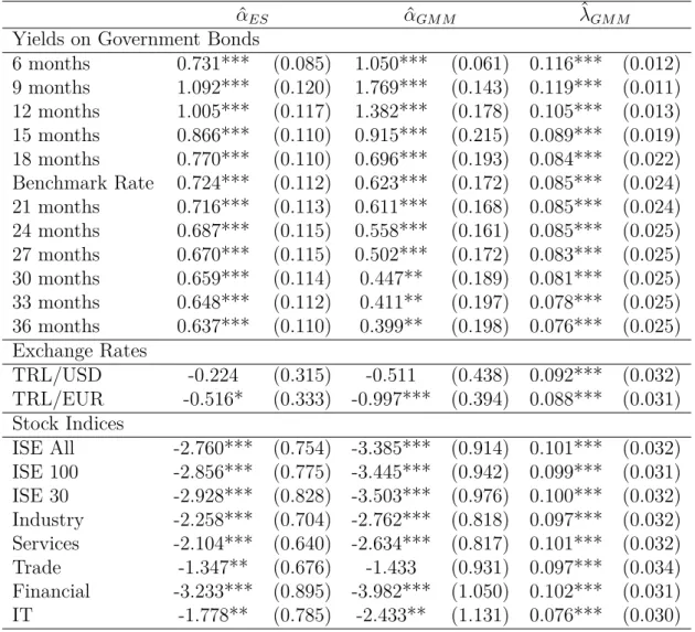
The fourth essay takes a different turn and measures the monetary policy transmission mechanism in Turkey. Quantifying the impact of policy decisions on financial markets is complicated because of the simultaneous response of policy actions to the asset prices, and possible omitted variables that both variables respond to. This chapter applies a heteroscedasticity-based general-ized method of moments (GMM) technique for financial markets in Turkey to overcome these problems. This approach is based on the heteroscedasticity of the policy surprises on monetary policy committee meeting dates to identify the financial market reaction to monetary policy. The findings are used as a cross-check for the widely-used identification technique, namely the OLS-based event study. The results suggest that event study estimates are biased for some asset returns.
Keywords: Endogenous Regime Switching, Inflation Expectations, Monetary
¨OZET
MAKROEKONOM˙I ¨UZER˙INE MAKALELER
¨Ozcan, G¨ulserimDoktora, ˙Iktisat B¨ol¨um¨u
Tez Y¨oneticisi: Prof. Dr. Refet Soykan G¨urkaynak Eyl¨ul 2017
Bu tez, parasal iktisat oda˘gında, makroekomi ¨uzerine d¨ort makaleden olu¸sup rasyonel olmayabilecek beklentileri uygulamalı ve teorik olarak ¸calı¸smaktadır. ˙Ilk makale, enflasyon beklentilerinin olu¸sturulmasında enflasyon deneyi-minin rol¨un¨u incelemektedir. Makale, farklı tahmincilerin enflasyon beklenti-lerinin ne ¨ol¸c¨ude ikamet ettikleri b¨olgede ger¸cekle¸sen enflasyondan etkilendi˘gini ara¸stırmaktadır. ¨Ozellikle farklı ¨ulkelerdeki profesyonel tahmincilerin Avro b¨olgesi enflasyon tahminlerine odaklanılarak, bu tahmincilerin tahmin hata-ları ile ikamet ettikleri ¨ulkelerde g¨ozlemlenen enflasyon arasındaki ili¸ski am-pirik olarak incelenmi¸stir.
¨Oncelikle, ana ¨ulkedeki ger¸cekle¸sen enflasyon oranı arttık¸ca, tahmincilerin, Avro b¨olgesi enflasyon beklentilerini yukarı y¨onl¨u g¨uncelledikleri ve bunun da daha yu¨uksek, tahmin edilebilir tahmin hatalarına yol a¸ctı˘gı g¨osterilmi¸stir. Bu bulgu tahmincilerin Avro b¨olgesini kendi ¨ulkelerine oldu˘gundan fazla ben-zetmesinden veya her yerde enflasyonun ger¸cekte oldu˘gunda daha g¨u¸cl¨u bir ¸sekilde otokorele oldu˘gunu d¨u¸s¨unmelerinden kaynaklanıyor olabilir. Y¨ur¨ut¨ulen
testler sonucunda tahmincilerin, enflasyonun mekansal boyutunu do˘gru bir ¸sekilde anladıkları fakat zamansal olarak hata yaptıkları kanıtlanmı¸stır. Tah-minciler, d¨unyayı -hem kendi ¨ulkeleri hem de di˘ger ¨ulkeler i¸cin- oldu˘gundan daha fazla ardı¸sık ba˘gıntılı olarak algılamaktadırlar. Bu da belirgin bir ¸sekilde tahminedilebilen tahmin hatalarına yol a¸cmaktadır.
˙Ikinci makale, belirsizli˘gin Yeni Keynesyen modellerde amplifikasyon mekaniz-masını nasıl etkiledi˘gini ara¸stırmaktadır. C¸alı¸smada belirsizlik kavramı robust (sa˘glam) kontrol teorisi ile ele alınmı¸stır. Sa˘glam kontrol teorisine g¨ore, bir politika yapıcı aklındaki yapısal ekonomik ba˘gıntıların hatalı olabilece˘ginden endi¸se ediyorsa para politikasını belirlerken olası en k¨ot¨u senaryoya g¨ore hareket ederek sa˘glam sonu¸clar ¨uretmeyi hedefler. Tezin bu b¨ol¨um¨unde, fiyatların yapı¸skan oldu˘gu Keynesyen bir modelde belirsizli˘gin etkisi ¸calı¸sılmı¸stır. Bu modelde, optimal para politikasının talep ¸sokuna kar¸sı, belirsizli˘gin olmadı˘gı duruma kıyasla daha aktif bir duru¸s sergiledi˘gi bulunmu¸stur. ¨Ote yandan, lit-erat¨urdeki genel kanının aksine, para politikasının arz ¸soku kar¸sısındaki duru¸su belirsizlik altında zayıflamaktadır. Ayrıca, modele endojen kalıcılık (endoge-nous persistence) mekanizmaları ilave edildi˘ginde, para politikasının etkinli˘gi zayıflayaca˘gından politikanın daha da agresif bir hale gelmesi gerekir. Fakat ekonomik birimlerin fayda fonksiyonunda makul d¨uzeyde t¨uketim alı¸skanlıklarına yer verildi˘ginde, belirsizli˘gin arz ¸soku kar¸sısında bile daha atılgan bir politikaya yol a¸ctı˘gı g¨or¨ulm¨u¸st¨ur.
¨U¸c¨unc¨u makalede, ekonomide para politikası aktarımının zayıflayaca˘gı bir rejim de˘gi¸sikli˘gi olasılı˘gı oldu˘gunda optimal para politikasını nasıl belirlendi˘gi ara¸stırılmaktadır. C¸alı¸smanın amacı, rejim de˘gi¸sikli˘gi ihtimalinden do˘gan
bek-lentisel etkilere vurgu yapmaktır. Olu¸sturulan model ¸cer¸cevesi, para poli-tikası etkinli˘ginin zayıflaması riskinin politika yapıcını davranı¸slarına etkisi ayrı¸stırılmasına olanak vermektedir. C¸alı¸sma sonu¸clarına g¨ore, merkez bankası gelecekteki etkinli˘gin azalmasına kar¸sı ¨onlem almak amacıyla, normal zaman-larda dahi daha aktif bir duru¸s sergilemektedir.
D¨ord¨unc¨u makalede, T¨urkiye’de para politikası aktarımı ¨ol¸c¨ulmektedir. Geli¸smekte olan ¨ulkelerde, para politikasının varlık fiyatlarına etkisi hakkında pek az bilgi mevcuttur. Para politikasının etkisinin ¨ol¸cu¨ulmesi, politika hareket-lerinin ve varlık fiyatlarının e¸szamanlı tepkisi ve her iki de˘gi¸skenin dahil edilmeyen ba¸ska de˘gi¸skenlere tepki vermesi ihtimali nedeniyle karma¸sıkla¸sır. Bu b¨ol¨um, bahsi ge¸cen sorunları ¸c¨ozmek i¸cin, de˘gi¸sken varyansa dayalı genelle¸stirilmi¸s mo-mentler y¨ontemini T¨urkiye’deki finansal piyasalara uygulamı¸sır. Bu y¨ontem, finansal piyasaların para politikasına tepkisini ¨ol¸cmek i¸cin, politika ¸sokunun para politikası kurulu toplantı g¨unlerindeki de˘gi¸sen varyansına dayanır. Sonu¸clar literat¨urde yaygın olarak kullanılan vaka ¸calı¸sması ile kar¸sıla¸stırmalı olarak sunulmu¸stur. Sonu¸clar, bazı varlık getirileri i¸cin ¨onceki tahminlerde istatistik-sel olarak bir miktar sapma oldu˘gunu g¨ostermektedir.
Anahtar Kelimeler: Belirsizlik, Endojen De˘gi¸sken Rejim, Enflasyon
ACKNOWLEDGEMENTS
This thesis would not have been possible without the inspiration and sup-port of many wonderful people. My thanks and appreciation to all of them for being part of this journey.
First and foremost, I would like to express my deepest gratitude to Refet S. G¨urkaynak, for his invaluable guidance, exceptional supervision, support and encouragement throughout all stages of my graduate study. I am immensely grateful to him. It is no doubt that working with him made a difference in my professional life as well as my personality.
During my visiting studies at the DIW (German Institute for Economic Research) Berlin, I was fortunate to work with Marcel Fratzscher to whom I must offer my profoundest gratitude.
It would be impossible to overstate my gratitude to Sang Seok Lee for his valuable comments, insights, constant faith in my work and making time for me whenever I needed in my last year. I would like to thank Levent Akdeniz, Ay¸se Kabuk¸cuo˘glu and Pınar Derin G¨ure, who are the examining committee members, for their suggestions. I also wish to thank to all of the professors at the Department of Economics for their support and guidance throughout my graduate years at the department. I need to mention ¨Ozlem Eraslan and Nilg¨un C¸orap¸cıo˘glu for making their support available in a number of ways.
The financial support of T¨UB˙ITAK during my studies is gratefully ac-knowledged.
It is a pleasure to thank my friends Ay¸se G¨ul Mermer, Sevilay Bulut, Seda K¨oymen, ¨Omer Faruk Akbal, Zeynep Kantur, Seda Meyveci, Burcu Fazlıo˘glu, Sırma Kollu, Deniz Yıldırım, G¨une¸s Kolsuz, Elif ¨Ozcan, Anıl Ta¸s, G¨ok¸ce Kara-soy and S¨umeyra Korkmaz for their sincere friendship and and making my graduate life easier. Thank you, Ay¸se G¨ul again, I am grateful for your ever-lasting friendship in good and bad days along all these years.
Finally, my deep and sincere gratitude to my parents G¨ulsen and Do˘gan, and my sister G¨ul¸sah for their endless encouragement and continuos love, and without which I would not have come this far. This journey would not have been possible if not for them, and I dedicate this milestone to them.
TABLE OF CONTENTS
ABSTRACT . . . . iii ¨ OZET . . . . vi TABLE OF CONTENTS . . . . xi LIST OF TABLES . . . . xvLIST OF FIGURES . . . xvii
CHAPTER 1: INTRODUCTION . . . . 1
CHAPTER 2: INFLATION EXPERIENCE AND INFLATION EXPECTATIONS: SPATIAL EVIDENCE . . . 9
2.1 Data . . . 13
2.1.1 Evaluation of Mean Forecast Errors . . . 16
2.2 Methodology and Results . . . 17
2.2.1 Corrupting Effect of Home Inflation . . . 18
2.2.2 The Effect of a Global Common Factor . . . 21
2.2.3 Alternative Measures of Global Inflation . . . 23
2.2.4 EA Inflation, World Inflation and Interaction Effects . . 25
2.4 Conclusion . . . 27
CHAPTER 3: THE AMPLIFICATION OF THE NEW KEY-NESIAN MODELS AND ROBUSTLY OPTI-MAL MONETARY POLICY . . . . 34
3.1 Motivation . . . 34
3.2 Optimal Monetary Policy . . . 38
3.2.1 Microeconomic Foundations of the Benchmark Model . . 40
3.2.2 Optimal Commitment Policy under Rational Expectations 43 3.2.3 Introducing Uncertainty . . . 44
3.2.4 Robust Monetary Policy Under Discretion . . . 49
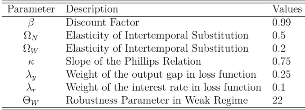
3.2.5 Calibration . . . 52
3.2.6 Impulse Responses . . . 55
3.2.7 Comparison with the Literature . . . 60
3.3 Introducing Endogenous Persistence to the Model . . . 62
3.3.1 Habit Formation in Consumption . . . 63
3.3.2 Backward-looking Firms . . . 66
3.3.3 Habit Formation and Inflation Persistence . . . 68
3.3.4 Comparison with the Literature . . . 72
3.3.5 Impulse Responses . . . 74
3.4 Conclusion . . . 80
CHAPTER 4: OPTIMAL MONETARY POLICY WITH A FEAR OF A CHANGING ECONOMIC STRUCTURE UNDER UNCERTAINTY . . . . 82
4.1 Introduction and Background . . . 82
4.2 Model . . . 90
4.2.1 Solution Methods via Deterministic Switching versus Regime Switching . . . 92
4.3 Results . . . 95
4.3.1 Piecewise Linear Solution . . . 96
4.3.2 Regime Switching . . . 97
4.4 Discussion of Policy Implications and Future Work . . . 101
CHAPTER 5: MEASURING THE IMPACT OF MONETARY POLICY ON ASSET PRICES IN TURKEY . 103 5.1 Introduction . . . 103 5.2 Methodology . . . 104 5.2.1 Data . . . 106 5.2.2 Empirical Results . . . 106 5.3 Conclusion . . . 110 REFERENCES . . . 111 APPENDICES . . . 120 A Data Appendix . . . 120 B Model Derivation . . . 122
C Solution Algorithm for the Approximating Equilibrium . 127 D State-space representation of New Keynesian models . . 130
F Solution Algorithms for Deterministic Switch versus Regime Switch . . . 140
LIST OF TABLES
2.1 The Effect of Home Inflation (FE) . . . 18
2.2 The effect of home inflation- Decomposing the Dependent Variable 19 2.3 Spatial Dimension . . . 20
2.4 Temporal Dimension I . . . 20
2.5 Temporal Dimension II . . . 21
2.6 The Effect of Global Inflation . . . 22
2.7 Alternative Measures of Global Inflation . . . 23
2.8 Correlation Matrix of Alternative Measures of Global Inflation . 24 2.9 EA Inflation, World Inflation and Interaction Effects . . . 26
2.10 EA and World Inflation rates- Decomposing the Dependent Variable . . . 29
2.11 Before-During-After the Crisis . . . 30
2.12 In the EA- Out the EA . . . 31
2.13 In the EA: Before-During-After the Crisis . . . 32
2.14 Out the EA: Before-During-After the Crisis . . . 33
3.1 The Benchmark Model . . . 43
3.2 Benchmark Calibration . . . 52
3.4 The Impact of Uncertainty on the Policy under Discretion . . . 56
3.5 Consumption Habits . . . 63
3.6 Inflation Persistence . . . 66
3.7 Inflation and Habit Persistence . . . 69
3.8 Calibration . . . 72
3.9 The Impact of Uncertainty on the Policy Rule . . . 73
4.1 Calibration . . . 96
5.1 Estimation Results . . . 107
LIST OF FIGURES
2.1 The timing of releases . . . 15
2.2 Mean Forecast . . . 16
2.3 Spatial Dimension versus Temporal Dimension . . . 19
2.4 Interaction Effects . . . 27
3.1 Impulse Responses of the Benchmark Model Under Uncertainty 57 3.2 Benchmark Model- Commitment versus Discretion . . . 61
3.3 Comparison with Giordani and S¨oderlind (2004) . . . 62
3.4 Impulse Responses under Rational Expectations . . . 75
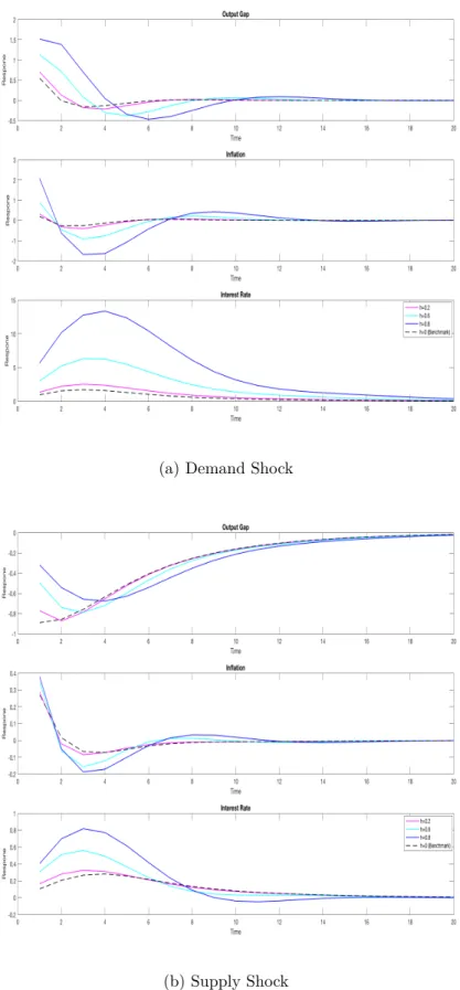
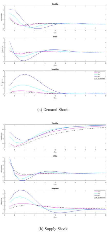
3.5 Impulse Responses for the Demand Shock . . . 78
3.6 Impulse Responses for the Supply Shock . . . 79
4.1 Impulse Responses for Piecewise Linear Solution-Demand Shock 98 4.2 Impulse Responses with exogenous transition probabilities . . . 99
4.3 Impulse Responses with endogenous transition probabilities . . . 100
1 Degree of Habit Persistence Under Rational Expectations . . . . 136
2 Degree of Habit Persistence Under Uncertainty . . . 137
3 Degree of Inflation Persistence Under Rational Expectations . . 138
CHAPTER 1
INTRODUCTION
Understanding inflation expectations is an integral part of understanding asset pricing and real economic decisions. Central banks try hard to control inflation expectations as these affect behavior and inflation outcomes.
Although most macroeconomic models rely on rationality of economic de-cision makers, empirical evidence generally reject rational expectations hy-pothesis. Theoretically, departures from rational expectations hypothesis in several ways is extensively studied in the literature. Adaptive learning, ra-tional inattention, noisy or sticky information and other forms of behavioral explanations are possible approaches to model bounded rationality. Yet, dif-ferent modelling strategies have difdif-ferent implications and predictions on the dynamics of macroeconomic variables. Hence, it is imperative to understand the expectation formation process.
The first essay of the thesis (Chapter 2) contributes to the line of research on how expectations are formed and how they deviate from the rational pectations hypothesis. This essay empirically studies the role of inflation
ex-perience in the formation of inflation expectations in the euro area by using a survey of professional forecasters. The study investigates whether and to what extent inflation expectations of different forecasters are affected by the inflation they observe in the country they are residing in. To test whether personal experiences play a role in deriving possible deviations from rational-ity, this chapter focuses on the expectations of professional forecasters from different countries of euro area inflation and asks whether their forecast errors are correlated with the observed inflation in the forecaster’s country at the time the expectation was formed. The essay documents a significant correla-tion between home country inflacorrela-tion and euro area inflacorrela-tion forecast error for the next year. Following up on this finding, the forecast error is decomposed into a spatial error in which forecasters think euro area is more like their own country than it actually is, and a temporal error in which forecasters perceive inflation is more strongly auto correlated everywhere than it actually is. We find that the source of the forecast error is exclusively in the temporal dimen-sion. Forecasters perceive the world to be more (positively) serially correlated than it actually is not only for their own country but also for other countries. Surprisingly, they get the spatial correlation right. To further elaborate the temporal dimension, a global common factor is used in explaining the forecast errors and the result that temporal dimension is the only source of the forecast error is confirmed.
The first essay shows that professional forecasters make systematic errors when forecasting euro area inflation. The expectations of the private agents translates into their actions which determines the effectiveness of the monetary
policy. This is how the first part of the thesis relates to the theoretical essays in which alternative assumptions to rational expectations on expectation for-mation of decision makers is embraced under uncertainty.
Awareness of the uncertainties regarding the structure of the economy might lead to shifts in the expectation formation of economic agents, and call for fundamental changes in the way policy is conducted. Certainty equiva-lence principle prescribes an optimal policy that is independent of uncertainty given the expected values of all state variables. However, uncertainty might reveal itself in many different forms that might cause violations of certainty equivalence. Policy makers seek policies that are robust across different (un-certain) states of the world, and optimality of the decision rules necessitates minimizing the impact of any type of uncertainty. How best to react to un-certainty, depending on its different forms, is widely studied by academics to provide guidance for policymakers.
Future paths of exogenous additive errors to the structural equations of the economy are uncertain from the perspective of the policymaker. To deal with these stochastic shocks as additive uncertainty, policy instruments are optimally prescribed to be set as if there were no uncertainty.1
A more sophisticated form of uncertainty is when the policymaker is uncer-tain about the effects of the policy. In this case, optimal choice of the policy variable will depend on the amount of uncertainty underlying the parameter in question as first pointed out by the seminal work of Brainard (1967). Put differently, this type of uncertainty is multiplicative with respect to the policy
1In a linear-quadratic setting, that is when the structure of the economy is represented
by linear equations and the objective function of the policymaker is quadratic, certainty equivalence principle applies.
variable. In such an environment, certainty equivalence does not hold so that a cautious/gradual/attenuated/conservative policy stance is able to optimally repress the effects of uncertainty.
Another example of multiplicative uncertainty is concerned with dynamic responses to shocks. When a policymaker is not sure about the impact of current values of the variables on future values, optimal policy requires reacting more actively/aggressively to keep the current variables stable as suggested by Giannoni (2002) among others. Clearly, caution is not always desirable; and in some cases, aggressiveness is more effective in reducing the effect of uncertainty. A more general form of uncertainty is when the policymaker faces general
model uncertainty. When the policymaker can put a structure on the model
uncertainty, she can assign prior probabilities to possible different views of the economy. To design a robust policy across competing models, a policymaker first computes economic losses implied by optimal policy prescribed by each model. And she minimizes average expected loss across models, in which the policymaker assigns larger weights for most likely model and smaller weights for least likely model. Hence, she utilizes Bayesian model averaging to insure against undesirable outcomes (as in Levin et al. (2003)). A robust policy under structured model uncertainty is set to work well across alternative models.
On the other extreme, the policymaker might face unstructured uncertainty when she cannot assign probabilities to alternative models of the economy. In this case, policymaker has a reference model of the economy; however, she has doubts about her model and thinks that her model can only approximate the structure of the economy. These are robust control problems.
To accommodate potential model misspecification, she considers a set of alternative models that are difficult to distinguish from her reference model. Decision-making under robust control can be interpreted as a dynamic game between the policymaker and the nature. In this game, nature, or the hypo-thetical evil agent forms the worst-case strategy for the policymaker, and the policymaker designs the best decision rule given the decision of nature. Hence, a robust policymaker seeks a max-min solution, which maximizes the worst outcome to the policy problem. This type of uncertainty is additive and is reflected as additional disturbances, which can feed back on state variables, in the additive shock processes.
As opposed to structured model uncertainty,2 the robust control approach
relies on designing optimal policy that would work on the worst possible out-come irrespective of how (un)likely this outout-come might be. Hence, in the case of designing robust policy under unstructured uncertainty, policymaker has to set a prior judgment on the worst-case outcome depending on how much she is concerned about model misspecification. Hansen and Sargent (2008) sug-gest interpreting possible deviations from policymaker’s reference models as a collection of the likelihood ratios whose relative entropies with respect to the reference model are bounded by the policymaker’s desired degree of robustness. This thesis aims to provide an analytical understanding of the effects of uncertainty by dissecting the optimal behavior of the monetary authority in forward-looking models. The second part of the thesis is theoretical. The second essay of this thesis (Chapter 3) analyzes whether and how model
un-2See Kara (2002); Giannoni (2002) for examples of a comparison of structured and
certainty affects the amplification mechanism of the New Keynesian models by providing a comparison of the dynamics of the models under rational expecta-tions and under model uncertainty under the optimal commitment policy. On modeling uncertainty, this chapter explicitly relies on the robust control liter-ature. I find that the impact of uncertainty on the monetary policy depends on the type of the shock as well as model features.
While being intuitive, the study presents some attracting findings on the optimal policy with a concern for robustness to model misspecification in New Keynesian models. First, the concerns about model uncertainty always make the policymaker attribute less importance to nominal interest rate inertia. Second, the reaction of the policymaker to a demand shock always becomes stronger, i.e. more aggressive, under in the presence of habit formation. The monetary authority reacts aggressively to prevent the fluctuations in marginal utility of the households. However, persistence in inflation smooths out the fluctuations in output, and partially dampens the impact of model uncertainty. Third, the results show that supply shock is more persistent under model uncertainty. Yet, the initial response of the policymaker depends on the type of the model. The models taking habit persistence into consideration calls for an aggressive policy. The policymaker keeps the policy rate lower at first compared to the case under rational expectations for the benchmark model and the model with inflation persistence.
The third part of the thesis (Chapter 4) analyzes theoretically the potential effects of the fear of a changing economic structure on optimal monetary policy. In a world where the presence of an effective lower bound on nominal interest
rate weakens the ability of the central bank in offsetting shocks and stimulating the economy, conducting economic policies that will serve as buffers against this risk becomes relevant.
In this chapter, I allow for regime-dependent elasticity of substitution as a short-cut to model a possible weakening of monetary policy effectiveness subject to an effective lower bound on nominal interest rate. In an environment where the central banker is not able to use her conventional instrument, she has to rely on alternative channels. Although, theoretically, the monetary authority has other, unconventional, tools such as forward-guidance and asset purchase programs to effect the real economy, these tools are proven not to work uniformly well in practice. Hence, alternating states of the economy where monetary authority is forced to switch to unconventional tools is similar to the economic environment in this study especially when unconventional tools do not work as well as the standard policy tool.
The findings of this chapter suggest that awareness of the possibility of hitting the bound leads to shifts in the expectation formation of the private agents, and call for fundamental changes in the way policy is conducted even before the bound has been reached. This study will provide insights for pol-icymakers trying to stimulate the demand and weaken the effects of deep re-cessions when the constraint on nominal interest rate may bind. The study combines both risk and model uncertainty by allowing for alternating states of the economy. The results of the chapter first demonstrate that weakening of the monetary policy transmission mechanism calls for stronger policy ac-tions in response to shocks in the good state as well. That is, when agents
acknowledge this possible future change in the economic structure, optimal policy becomes more active in normal times as well as near the effective lower bound.
The fourth essay constitutes the final chapter of the thesis and is included to fulfill the publication requirement. The chapter estimates the monetary policy transmission mechanism in Turkey using an identification mechanism that works through the heteroscedasticity in the high-frequency data.
Overall the contributions of this thesis are; first, providing evidence on how the expectation formation of survey respondents deviates from rational expectations. Second, it adds to the theoretical literature on the interaction of guarding against model uncertainty and model features of the forward-looking dynamic stochastic general equilibrium models. Third, it contributes to the literature where optimal policy is analyzed under possible monetary policy regime switches, and by extending the existing analyses for an environment where optimal behavior of the monetary authority is constructed when uncer-tainty aversion increases with weakening monetary policy transmission. With the help of sophisticated modelling techniques, the study provides policy rec-ommendations for optimal policy conduct.
CHAPTER 2
INFLATION EXPERIENCE AND
INFLATION EXPECTATIONS: SPATIAL
EVIDENCE
Understanding inflation expectations is an integral part of understanding asset pricing and real economic decisions. Central banks try hard to control inflation expectations as these affect consumption, spending and investment behavior of economic agents and inflation outcomes.
Measuring expectations via surveys is common but the literature shows that survey responses do not reflect rational expectations: survey forecast errors are often forecastable. In particular, Malmendier and Nagel (2016), using the Michigan Survey of household expectations, show that average inflation people experience during their formative years continue to color their expectations decades later and Andrade and Bihan (2013) show that European forecasters make systematic errors in forecasting euro area inflation. A recent survey experiments recorded by Cavallo et al. (2017) demonstrate that consumers form inflation expectations using their memories of supermarket prices.
expecta-tions, for instance, Evans and Honkapohja (2001) suggests the adaptive learn-ing to model bounded rationality.1 Further, rational inattention literature
shows how the dynamics of macroeconomic variables are affected when agents have to allocate limited attention to macroeconomic information (Sims, 2003; Reis, 2006; Ma´ckowiak and Wiederholt, 2009, 2015). Other forms of infor-mational rigidities are considered via noisy or sticky information (Woodford, 2003; Mankiw and Reis, 2002). Coibion and Gorodnichenko (2012, 2015) em-pirically test how agents’ forecast errors respond to structural shocks, and how they are related to past forecast revisions as implied by imperfect information models.
A new line of the literature takes a different stance in explaining expec-tation formation of economic agents. Among many others, Gabaix (2016) uses an application of sparsity approach in providing behavioral explanations. Bhandari et al. (2016) identifies possible diversions from rationality by devi-ations of consumer survey expectdevi-ations from those of professional forecasters, and justify this departure in an environment where agents form expectations relying on the worst-case model with concerns about model misspesification.
It would have been easy to write off these pathologies of survey expecta-tions as reflecting careless or strategic answers or unsophisticated respondents who may not matter at the margin but Ang et al. (2007) argue that survey expectations of inflation are the best forecasts of inflation. More recently, Croushore (2010) and Faust and Wright (2013) provide evidence that surveys of professional forecasts perform better when compared to several statistical
1See Evans and Honkapohja (2009) for a survey of the literature on adaptive learning
and theoretical model-based forecasts. Further, a lot of ”puzzles” in macroeco-nomics are alleviated when survey expectations are used in models instead of model consistent (rational) expectations. Piazzesi and Schneider (2008) show that understanding the yield curve becomes much easier if survey expectations are used instead of model consistent expectations. Fuhrer (2012) shows the same for the fit of DSGE models by replacing rational expectations with survey expectations since these eliminate the need for adding ad hoc model features such as habit formation and inflation indexation which has limited support in the micro data, and complex error processes to match the dynamic properties of macro data.
Recent studies support the empirical validity of inflation expectations sur-veys by documenting that sursur-veys are informative about economics decisions. By using a financially incentivized experiment about investment decisions of households, Armantier et al. (2015) shows that consumers tend to act on their beliefs about future inflation. D’Acunto et al. (2015) finds that German households’ willingness to purchase increases with their inflation expectations. Hence, survey expectations matter and it is imperative to understand how they are formed, how exactly they deviate from rational expectations.
The goal of this study is to investigate the role of inflation experience in the formation of inflation expectations by investigating whether and to what extent inflation expectations of different forecasters are affected by the inflation they observe in the country they are residing in.
We use a novel data set by Consensus Economics. We exploit the fact that many forecasters provide forecasts of the euro area inflation and these
forecasters are in different firms, located in different countries. Hence there is a spatial dimension in the inflation experience of the forecasters. Thus, we focus on the expectations of professional forecasters from different countries of euro area inflation and ask whether their forecast errors are correlated with the observed inflation in the forecaster’s country at the time the expectation was formed.
The role of geography in explaining the forecast heterogeneity and disagree-ment among forecasters is explored in the literature.2
We find that a significant correlation between home country inflation and euro area inflation forecast error for the next year. We devise tests to de-compose the forecast error into i) a spatial error in which forecasters think euro area is more like their own country than it actually is, and ii) a temporal error in which forecasters perceive inflation is more strongly auto correlated everywhere than it actually is. We document that the source of this error is mostly the temporal dimension. Forecasters perceive the world to be more (positively) serially correlated than it actually is for their home country as well as for other countries. They get the spatial correlation right. To further elaborate the temporal dimension, we empirically test the explanatory power of a global common factor in explaining the forecast errors. With several al-ternative measures of global inflation, we confirm our initial results that the temporal dimension is the source of the forecast error.
Lately, the relationship between global economic conditions and forecasting
2For instance, see Berger et al. (2008) show that predictions about monetary policy
exhibit a significant and systematic regional pattern in the Euro Area and forecast errors of the forecasters are larger as economic developments in their home region differs from the average. Berger et al. (2006) document the same for American professional forecasters.
domestic inflation has drawn attention in the literature.3 Ciccarelli and
Mo-jon (2010) and Kabuk¸cuo˘glu and Mart´ınez-Garc´ıa (2016) are example studies documenting the comovement of individual countries’ inflation and help under-stand the role of global inflation in the prediction of local inflation. Moreover, Kearns (2016) dissects the exact opposite angle by studying the predictive power of survey expectations of domestic inflation on the global inflation.4
All aside, this is the first study documenting the global factors behind the misperceptions regarding inflation expectations.
The remaining of the paper proceeds as follows. Section 1 describes the Consensus Economics data, section 2 describes the methodology used and studies the results, while section 3 concludes.
2.1 Data
The analysis is carried out using monthly data for annual inflation expecta-tions for the current and the next calendar year. The data source for inflation expectations is Consensus Economics database, and realized inflation rates are from IMF International Financial Statistics (IFS). Consensus Economics asks professional forecasters from different firms residing in different countries for their forecasts of a large number of variables at the beginning of each month. Respondents of the survey are commercial/investment banks, forecast compa-nies, and research institutes.
3While Edge et al. (2010) provides a comparison of the forecast performance of many
statistical, judgmental and Dynamic Stochastic General Equilibrium models. Including a global, open economy dimension improves forecast performance substantially.
4They contradict with the literature and show that global inflation does not improve
the survey forecasts of domestic country inflation, suggesting that survey forecasters have historically already incorporated information on global inflation in their forecasts.
In our analysis, we use the Euro Area consumer price inflation forecast of these institutions. Consensus Economics survey asks the respondents about their end-year inflation forecasts for the current year and the following year at a monthly frequency. Hence, respondents forecast the same annual inflation throughout the year. This monthly data/calendar year fixed-event forecast creates an MA(11) error term.5 For instance, next year forecasts collected in
January 2008 are for the calendar year 2009 that will begin in 12 months, whereas those in February 2008 are for the same calendar year, which will now begin in 11 months.
To obtain forecasts with a fix horizon of one year ahead, following Celasun et al. (2004) we define one-year-ahead forecasts as a weighted average of the forecasts of the current and the next calendar year as follows:
Definition 1. For each monthly date t, in month m of the year, twelve-month ahead forecast ft+12,tis a weighted average of the end-year forecasts for current
year ft+(12≠m),t and the end-year forecasts for next year ft+(24≠m),t:
ft+12,t= (12 ≠ m)(ft+(12≠m),t
) + m(ft+(24≠m),t)
12
Each year, in month m, current year forecast has a forecast horizon 12≠m; and next year forecast has a 24 ≠ m forecast horizon. Moreover, the twelve-month ahead forecast has 12 ≠ m twelve-months in the current calendar year, and m months in the following year, which constitutes the shares of the current and the next year forecasts.
5We do a robustness check by using only data from January observations. A detailed
We construct the forecast error as the difference between the actual inflation for the next year and the forecast that was provided in the current month as follows:
Definition 2. For each monthly date t, twelve-month ahead forecast error of forecaster i is the realized monthly year-over-year future inflation, fit+12, minus
twelve-month ahead forecast of forecaster i, ft+12,it:
f ei,t = fit+12≠ ft+12,it (2.1)
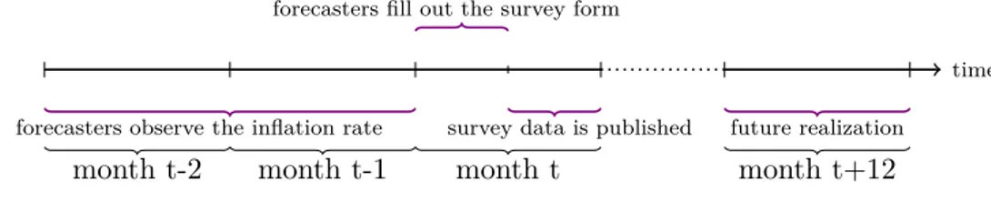
The timing of releases is summarized in the following figure: Figure 2.1: The timing of releases
time
month t-2 month t-1 month t month t+12
forecasters observe the inflation rate
forecasters fill out the survey form
survey data is published future realization
We assume that forecasters have not observed inflation for the month when the survey came out, and it is possible that in some countries the forecasters have not yet seen the official release of inflation for the previous month by the time they provide their forecasts; thus, (publicly available) realized inflation at the time of the forecast belongs to two months before.6
To carry out the analysis, we assign home countries for each professional forecaster based on the location of the headquarters of their firms. These professional institutions are from 14 different countries from which Austria,
6One can argue that even though forecasters have not seen the inflation for the previous
month, they have experienced that inflation. The results of the paper is robust to using one-month lagged inflation as well.
Finland, France, Germany, Italy, Netherlands and Spain are from the euro area, and Canada, Denmark, Norway, Sweden, Switzerland, United Kingdom and the United States are outside the euro area. Our panel data of 44 forecasters covers the period 2003:1-2012:12 with approximately 2500 observations.
2.1.1 Evaluation of Mean Forecast Errors
Even though we are interested in analyzing the micro properties of the inflation forecasts, it is imperative to study the mean forecasts to see whether it is comparable to different forecast data used in the literature. Mean forecasts and mean forecast errors together with their realizations are shown in the following figure.
Figure 2.2: Mean Forecast
Con-sensus Economics forecasters, on average, underestimated EA inflation. The only exception is 2009, the year following the financial crisis, in which aggre-gate demand collapsed sharply. Starting in 2010, mean forecast errors once again turned positive.
2.2 Methodology and Results
The goal of this study is to analyze the effect of inflation experience on the formation of inflation expectations. To empirically test the hypothesis that individual forecast errors of professional forecasters are correlated with home country inflation, we estimate the following fixed effect panel regression:
f eEAi,t = –i+ —fii,tHome≠2 + ‘i,t (2.2)
where feEA
i,t is the forecast error of forecaster i, in month t, –i denotes for the
forecaster fixed effect, and fiHome
i,t≠2 is the realized inflation in home country of
forecaster i available at the time of the forecast.
Equation (2.2) enables us to control for unobserved heterogeneity among forecasters. This method has the advantage of allowing for the existence of general patterns of correlation between the unobserved forecaster effects and euro area inflation forecasts.7
7We obtained very similar results from the pooled OLS regressions. We do not show
those results here, considering that the forecasters located in different countries may be different. Thus, the error term and location will be correlated and OLS will be biased.
2.2.1 Corrupting Effect of Home Inflation
As shown in Table 2.1, fixed effects panel regressions demonstrate a strong forecasting effect of home inflation on euro area inflation forecast errors. We use heteroskedasticity adjusted standard errors but the serial correlation in-duced by the monthly forecasts of annual inflation remains. A brute force method of controlling for this is to use forecasts made in one month of the year only8, which greatly reduces the sample size but makes sure that the MA
term is no longer present. The result remains statistically and economically significant and of similar magnitude across different specifications.
Table 2.1: The Effect of Home Inflation (FE)
Fixed Effects Fixed Effects (January)
EA 1-yr-ahead Fcast Error EA 1-yr-ahead Fcast Error
Lagged Home Inf -0.597*** -0.545***
(0.0833) (0.087) Constant 1.519*** 1.314*** (0.167) (0.169) Observations 2,595 201 R-squared 0.289 0.332 Number of panel id 44 37
Robust standard errors in parentheses *** p<0.01, ** p<0.05, * p<0.1
The negative coefficient suggests that when forecasters observe high home inflation they raise their forecasts of euro area inflation too much, so that the forecast error (realized minus forecasted inflation) is predictably low. This is in clear contradiction with rational expectations because forecast errors should not be predictable with any available information at the time of the forecast under rational expectations.
To understand the source of the strong forecasting effect of home inflation,
8The results are qualitatively the same for all months. We present the results for the
we decompose the dependent variable. Table 2.2 reports the responses of future EA inflation and expectations for next year’s euro area inflation. The results suggest that current home inflation and the future EA inflation are negatively correlated but forecasters perceive a positive correlation. This result may be due to both a spatial mistake in expectations formation and/or a temporal one.
Table 2.2: The effect of home inflation- Decomposing the Dependent Variable
Fixed Effects Fixed Effects (January) Fixed Effects Fixed Effects (January)
Realized Future EA Inf Forecasted Future EA Inf Lagged Home Inf -0.318*** -0.338*** 0.278*** 0.208***
(0.0592) (0.096) (0.030) (0.062) Constant 2.785*** 2.681*** 1.266*** 1.368*** (0.119) (0.186) (0.060) (0.120) Observations 2,595 201 2,595 201 R-squared 0.125 0.153 0.349 0.166 Number of panel id 44 37 44 37
Robust standard errors in parentheses *** p<0.01, ** p<0.05, * p<0.1
We find that current home inflation unduly affects expectations of next year’s euro area inflation, which may be because forecasters think euro area is more like their own country than it actually is (spatial) and/or think inflation is more strongly auto correlated everywhere than it actually is (temporal) as demonstrated by Figure 2.3. Hence, further elaboration is needed to separate these two channels.
Home next year EA next year
Home today EA today
To investigate which dimension the forecasters are missing, we first compare the correlation between the realized and the perceived home and EA inflation rates in Table 2.3 in order to test for the presence of spatial errors. In addition, we analyze the temporal dimension by comparing the correlation between the realized current and future EA inflation, and the correlation between perceived current and future EA inflation rates. Alternatively, we propose comparing the correlation between the realized current and future home country inflation, and the correlation between perceived current and future home country inflation rates.
Table 2.3: Spatial Dimension
Fixed Effects Fixed Effects
Current EA Inf EA Inf Forecast
Current Home Inf 0.655***
0.013
Home Inf Forecast 0.541***
(0.015)
Constant 4.153*** 3.191***
(0.020) (0.020)
Observations 2595 2595
Robust standard errors in parentheses *** p<0.01, ** p<0.05, * p<0.1
Table 2.4: Temporal Dimension I
Fixed Effects Fixed Effects
Realized Future EA Inf Forecasted Future EA Inf
Lagged EA Inf -0.466*** 0.478***
(0.029) (0.008)
Constant 5.006*** 3.003***
(0.020) (0.020)
Observations 2595 2595
Robust standard errors in parentheses *** p<0.01, ** p<0.05, * p<0.1
cor-Table 2.5: Temporal Dimension II
Fixed Effects Fixed Effects
Realized Future Home Inf Forecasted Future Home Inf
Lagged Home Inf -0.305*** 0.381***
(0.031) (0.014)
Constant 5.542*** 4.012***
(0.020) (0.020)
Observations 2595 2595
Robust standard errors in parentheses *** p<0.01, ** p<0.05, * p<0.1
relation of home and EA inflations is lower than it actually is; however the difference between these two is not statistically significant. Moreover, they per-ceive the correlation in the time dimension to be positive, whereas in reality is negative, which gives the overall negative coefficient. Thus, misperception comes from the temporal dimension so that forecasters perceive the world to be more (positively) serially correlated than it actually is, not only for their own country but also for other countries.
2.2.2 The Effect of a Global Common Factor
The dominance of the temporal mistake in the forecast error needs further elaboration. To empirically test the hypothesis that there is a time-varying global common factor driving the results, we conduct principal component analysis on the inflation rates in countries where the forecasters are residing in.9 The first common factor from the analysis is interpreted as the global
inflation rate that the forecasters experience.
We estimate equation (2.3) to analyze the effect of global inflation on the
EA inflation forecast error.
f eEAi,t = –i+ —1fii,tHome≠2 + —2fiGlobalt≠2 + ‘i,t (2.3)
where fiHome
i,t≠2 is the realized inflation in home country available at the time of
the forecast, and fiGlobal
i,t≠2 denotes for the global inflation available at the time
of the forecast.
Table 2.6: The Effect of Global Inflation
Fixed Effects Fixed Effects (January)
EA 1-yr-ahead Fcast Error EA 1-yr-ahead Fcast Error
Lagged Home Inf -0.037 -0.130*
(0.073) (0.059)
Lagged Global Inf -0.213*** -0.214***
(0.023) (0.016) Constant 0.447*** 0.536*** (0.142) (0.114) Observations 2,595 201 # of panel id 44 37 R-squared 0.441 0.597
Robust standard errors in parentheses *** p<0.01, ** p<0.05, * p<0.1
The results of the regression where we include the global inflation factor as well as home inflation as explanatory variables (summarized in table 2.6) are not surprising, and confirm our initial results that the temporal dimension is the source of the forecast error (This result favors the dominance of time series dimension). When we include the global inflation factor, home inflation is no longer statistically significant. Instead, global factor has a strong forecasting effect (-0.213, significant at the 1 percent significance level) on the EA inflation forecast error. These results put forward that, on average, forecasters signifi-cantly under-predict EA inflation by 213 basis points; and they increase their forecasts by approximately 100 basis points when they observe a 1 percent
increase in the global inflation factor.
2.2.3 Alternative Measures of Global Inflation
In the previous section, we document systematic errors in EA inflation fore-cast errors. Forefore-casts are correlated with the global inflation factor calculated by principal component analysis on individual country inflation rates. In this section, we analyze the alternative measures of global inflation. According to the Table 2.7, the predictive power of the global inflation measures calculated by the principal component analysis is lower than the other measures of global inflation.
Table 2.7: Alternative Measures of Global Inflation Pooled OLS
EA 1-yr-ahead Fcast Error
Lagged Home Inf 0.00222 -0.016 0.006 0.013
(0.0465) (0.052) (0.037) (0.052)
Lagged Global Inf -0.221***
(0.0164)
Lagged Global Inf2 -0.252***
(0.020)
Lagged EA Inf -0.896***
(0.057)
Lagged World Inf -0.817***
(0.053)
Constant 0.370*** 0.388*** 2.169*** 3.440***
(0.0826) (0.094) (0.066) (0.120)
Observations 2,595 2,595 2,595 2,595
R-squared 0.439 0.427 0.455 0.518
Robust standard errors in parentheses *** p<0.01, ** p<0.05, * p<0.1
Sources: World inflation and inflation for developed countries are from IMF. Global factor is the first component of the principal component analysis. Global factor2 is constructed as the weighted average of the first two principal components, where the weights are constructed as the share of the corresponding eigenvalue over the sum of the two relevant eigenvalues.
Table 2.8 documents the correlation matrix of alternative measures of global inflation. Alternative measures of global inflation are highly correlated with each other. We believe that the information on the global factors are
en-Table 2.8: Correlation Matrix of Alternative Measures of Global Inflation (1) inf ea m inf ea m 1 inf world m 0.899*** globalfactor 0.980*** globalfactor2 0.969*** homeinf m 0.675*** inf world m inf world m 1 globalfactor 0.950*** globalfactor2 0.956*** homeinf m 0.642*** globalfactor globalfactor 1 globalfactor2 0.998*** homeinf m 0.685*** globalfactor2 globalfactor2 1 homeinf m 0.679*** homeinf m homeinf m 1 N 2595 t statistics in parentheses * p < 0.05, ** p < 0.01, *** p < 0.001
compassed by the alternative measures. Our goal is to include all time-varying measures as much as possible in the analysis. To achieve that we will calculate the net contribution of each variable on the EA forecast error.10
We continue the analysis with EA inflation and the world inflation rates.11
2.2.4 EA Inflation, World Inflation and Interaction
Ef-fects
We estimate equation (2.4) to analyze the effect of global inflation on the EA inflation forecast error.
f eEAi,t = –i+ —1fitEA≠2+ —2‘tW orld≠2 + —3(fitEA≠2◊ ‘W orldt≠2 ) + ‘i,t (2.4)
where fiEA
t≠2 is the realized inflation in the EA available at the time of the
forecast, and ‘W orld
t≠2 denotes for the world inflation net of EA inflation available
at the time of the forecast, and (fiEA
t≠2◊ ‘W orldt≠2 ) is the interaction term between
the EA and world inflation rates.
Table 2.9 reports the results of the regression of one-year-ahead EA infla-tion forecast error on lagged EA inflainfla-tion and/ or world inflainfla-tion, and their interaction effects.12 Lagged EA inflation and world inflation rates have strong
forecasting effects on the EA inflation forecast error. On average, forecasters significantly under-predict EA inflation; and they increase their forecasts by
10The details of the calculation can be found in the appendix.
11The world inflation rate- net of EA inflation- is the residual from the regression of EA
inflation on the world inflation.
12Since we show that home inflation-the residual from the regression of home inflation on
EA and world inflation rates- is not statistically significant with time-varying global inflation measures, we do not report the results with the home inflation as an additional explanatory variable here.
Table 2.9: EA Inflation, World Inflation and Interaction Effects
EA 1-yr-ahead Fcast Error
Lagged EA Inf -0.895*** -0.868*** -0.702***
(0.0234) (0.022) (0.027)
Lagged World Inf -0.827*** -0.700*** 0.174***
(0.049) (0.029) (0.057)
(Lagged EA Inf x Lagged World Inf) -0.376***
(0.026) Constant 2.174*** 0.357*** 2.142*** 1.802*** (0.0483) (0.002) (0.045) (0.055) Observations 2,786 2,786 2,786 2,786 R-squared 0.456 0.101 0.528 0.539 Number of panel id 45 45 45 45
Robust standard errors in parentheses *** p<0.01, ** p<0.05, * p<0.1
more than 800 basis points in response to 1 percent increase in the EA in-flation/world inflation respectively. At the same time, the interaction term between these variables is negative and statistically significant at the 1 per-cent significance level. Negative interaction effects imply that the corrupting effect of EA inflation increases by world inflation. That is the effect of EA infla-tion gets stronger by approximately 400 basis points for higher levels of world inflation. Figure 2.4 illustrates the interaction effects between EA inflation and world inflation.
In order to analyze the source of the strong forecasting effect of EA and world inflation rates, we decompose the dependent variable. Table 2.10 reports the responses of future EA inflation and expectations for next year’s euro area inflation. The results suggest that current EA inflation together with world inflation rate and the future EA inflation are negatively correlated but forecasters perceive a positive correlation.
Figure 2.4: Interaction Effects
2.3 Robustness Checks
We separately analyzed pre-crisis and post-crisis periods. We find that cor-rupting effect of EA inflation weakens after the crisis. Although the behavior of inflation itself is mildly different, the behavior of inflation forecasts is not. Professional forecasters always perceive future euro area inflation to be more correlated with current inflation than it actually is. Moreover, the results are similar for euro area and non-euro area countries. However, forecasters from non-euro area countries make slightly larger forecastable errors.
2.4 Conclusion
In this paper, we study the impact of current inflation experience on ex-pectations of professional forecasters of euro area inflation with micro level data. We use a novel dataset which allows us to keep track of the evolution of
predictions regarding euro area inflation as well as home country inflation of individual forecasters.
Home inflation is significantly correlated with euro area (EA) inflation fore-cast error. We decompose this effect into i) spatial error, and ii) temporal error. We document that the source of this error is mostly the temporal dimension. They understand the spatial correlation correctly. The bottom line of this study is that forecasters perceive the world to be more serially correlated than it actually is for their home country, and for other countries as well.
Ta ble 2.1 0: E A and W or ld Infla tio n ra te s-D ec omp os ing the D ep ende nt Va ria ble Fc as t Fu tu re Fc as t Fu tu re Fc as t Fu tu re Fc as t Fu tu re Lagge d E A In f 0. 439*** -0. 456*** 0. 445*** -0. 423*** 0. 403*** -0. 299*** (0. 0143) (0. 016) (0. 014) (0. 012) (0. 015) (0. 019) Lagge d W or ld In f -0. 105*** -0. 933*** -0. 170*** -0. 871*** -0. 394*** -0. 221*** (0. 025) (0. 027) (0. 016) (0. 018) (0. 028) (0. 062) (Lagge d E A In fx Lagge d W or ld In f) 0. 096*** -0. 279*** (0. 014) (0. 026) C on st an t 0. 914*** 3. 088*** 1. 822*** 2. 179*** 0. 906*** 3. 049*** 0. 994*** 2. 796*** (0. 0295) (0. 034) (0. 001) (0. 001) (0. 029) (0. 025) (0. 031) (0. 039) O bs er vat ion s 2, 786 2, 786 2, 786 2, 786 2, 786 2, 786 2, 786 2, 786 R -s qu ar ed 0. 605 0. 181 0. 009 0. 197 0. 629 0. 351 0. 633 0. 361 Nu m be r of pan el id 45 45 45 45 45 45 45 45 R ob us t st an dar d er ror s in par en th es es *** p< 0. 01, ** p< 0. 05, * p< 0. 1
Ta ble 2.1 1: B ef or e-D ur ing -Af te r the C ris is (1) (2) (3) (4) (5) (6) (7) (8) (9) B ef or e D ur in g Af te r E A 1-yr Fc as t E rr or Lagge d E A In f -1. 312*** -1. 270*** -1. 069*** -1. 085*** -0. 916*** -0. 965*** -0. 208*** -0. 208*** -0. 015 (0. 0504) (0. 051) (0. 070) (0. 023) (0. 011) (0. 031) (0. 020) (0. 021) (0. 021) Lagge d W or ld In f 0. 454*** -1. 025*** -1. 314*** -1. 588*** -0. 022 0. 794*** (0. 033) (0. 332) (0. 053) (0. 185) (0. 043) (0. 047) (Lagge d E A In fx Lagge d W or ld In f) 0. 685*** 0. 106 -0. 523*** (0. 153) (0. 061) (0. 039) C on st an t 3. 269*** 3. 298*** 2. 867*** 2. 053*** 2. 184*** 2. 288*** 1. 284*** 1. 293*** 0. 983*** (0. 109) (0. 107) (0. 149) (0. 051) (0. 038) (0. 079) (0. 032) (0. 043) (0. 037) O bs er vat ion s 1, 478 1, 478 1, 478 732 732 732 576 576 576 R -s qu ar ed 0. 363 0. 386 0. 388 0. 604 0. 695 0. 695 0. 213 0. 214 0. 312 Nu m be r of pan el id 41 41 41 37 37 37 33 33 33 R ob us t st an dar d er ror s in par en th es es *** p< 0. 01, ** p< 0. 05, * p< 0. 1
Ta ble 2.1 2: In the E A-O ut the E A (1) (2) (3) (4) (5) (6) in th e E A ou t th e E A E A 1-yr Fc as t E rr or Lagge d E A In f -0. 874*** -0. 856*** -0. 688*** -0. 917*** -0. 881*** -0. 717*** (0. 0371) (0. 036) (0. 045) (0. 023) (0. 024) (0. 027) Lagge d W or ld In f -0. 681*** 0. 198* -0. 718*** 0. 146* (0. 034) (0. 083) (0. 043) (0. 074) (Lagge d E A In fx Lagge d W or ld In f) -0. 382*** -0. 368*** (0. 038) (0. 037) C on st an t 2. 107*** 2. 092*** 1. 746*** 2. 245*** 2. 195*** 1. 862*** (0. 0763) (0. 075) (0. 093) (0. 047) (0. 049) (0. 055) O bs er vat ion s 1, 433 1, 433 1, 433 1, 353 1, 353 1, 353 R -s qu ar ed 0. 453 0. 521 0. 533 0. 460 0. 536 0. 546 Nu m be r of pan el id 23 23 23 22 22 22 R ob us t st an dar d er ror s in par en th es es *** p< 0. 01, ** p< 0. 05, * p< 0. 1
Ta ble 2.1 3: In the E A: B ef or e-D ur ing -Af te r the C ris is (1) (2) (3) (4) (5) (6) (7) (8) (9) B ef or e D ur in g Af te r E A 1-yr Fc as t E rr or Lagge d E A In f -1. 287*** -1. 241*** -1. 076*** -1. 059*** -0. 911*** -0. 959*** -0. 214*** -0. 214*** -0. 004 (0. 0941) (0. 095) (0. 130) (0. 024) (0. 010) (0. 048) (0. 027) (0. 028) (0. 028) Lagge d W or ld In f 0. 478*** -0. 735* -1. 261*** -1. 530*** 0. 020 0. 883*** (0. 031) (0. 349) (0. 090) (0. 310) (0. 040) (0. 047) (Lagge d E A In fx Lagge d W or ld In f) 0. 562** 0. 104 -0. 565*** (0. 166) (0. 091) (0. 054) C on st an t 3. 189*** 3. 214*** 2. 862*** 1. 964*** 2. 117*** 2. 220*** 1. 275*** 1. 267*** 0. 932*** (0. 203) (0. 200) (0. 276) (0. 053) (0. 057) (0. 133) (0. 042) (0. 053) (0. 041) O bs er vat ion s 771 771 771 368 368 368 294 294 294 R -s qu ar ed 0. 357 0. 385 0. 386 0. 610 0. 693 0. 694 0. 232 0. 233 0. 348 Nu m be r of pan el id 22 22 22 19 19 19 16 16 16 R ob us t st an dar d er ror s in par en th es es *** p< 0. 01, ** p< 0. 05, * p< 0. 1
Ta ble 2.1 4: O ut the E A: B ef or e-D ur ing -Af te r the C ris is (1) (2) (3) (4) (5) (6) (7) (8) (9) B ef or e D ur in g Af te r E A 1-yr Fc as t E rr or Lagge d E A In f -1. 340*** -1. 302*** -1. 060*** -1. 112*** -0. 920*** -0. 972*** -0. 200*** -0. 201*** -0. 028 (0. 0209) (0. 016) (0. 054) (0. 033) (0. 021) (0. 045) (0. 035) (0. 035) (0. 032) Lagge d W or ld In f 0. 427*** -1. 342** -1. 362*** -1. 644*** -0. 069 0. 690*** (0. 063) (0. 503) (0. 050) (0. 229) (0. 065) (0. 051) (Lagge d E A In fx Lagge d W or ld In f) 0. 818** 0. 109 -0. 476*** (0. 232) (0. 088) (0. 059) C on st an t 3. 355*** 3. 388*** 2. 870*** 2. 148*** 2. 250*** 2. 357*** 1. 293*** 1. 318*** 1. 038*** (0. 0450) (0. 044) (0. 118) (0. 074) (0. 048) (0. 094) (0. 056) (0. 073) (0. 058) O bs er vat ion s 707 707 707 364 364 364 282 282 282 R -s qu ar ed 0. 368 0. 388 0. 391 0. 599 0. 696 0. 697 0. 194 0. 197 0. 278 Nu m be r of pan el id 19 19 19 18 18 18 17 17 17 R ob us t st an dar d er ror s in par en th es es *** p< 0. 01, ** p< 0. 05, * p< 0. 1
CHAPTER 3
THE AMPLIFICATION OF THE NEW
KEYNESIAN MODELS AND ROBUSTLY
OPTIMAL MONETARY POLICY
3.1 Motivation
Dynamic stochastic general equilibrium (DSGE) models combined with Bayesian methods of inference have become the mainstream device for research on mon-etary policy analysis. In its simple form,1 the model lacks endogenous
persis-tence than those present in the data. To improve the match with the data, many types of shocks together with adjustment costs are introduced into the model.2 Yet, in complex, elaborate DSGE setups containing several frictions,
some of these shocks are hard to validate.3
From the perspective of a policymaker, a highly related discussion would be acknowledging the possible uncertainties about the structure of the econ-omy. When one deviates from the assumption of perfect knowledge in several
1See Woodford (2011) and Gal´ı (2015) for the basic setup.
2See Smets and Wouters (2007), Fern´andez-Villaverde and Rubio-Ram´ırez (2006), and
Fern´andez-Villaverde (2009) for a medium-scale model.
ways, the propagation of shocks, hence implied policy suggestion could change substantially. For instance, although the literature on uncertainty pioneered by Brainard (1967) advised more cautious behavior for the policymaker when faced with ambiguity about parameters of the model, there may be fundamen-tal uncertainties regarding the true data generating process. The monetary authority facing uncertainty about the model or about the exogenous distur-bances might find it optimal to respond aggressively to fluctuations in the economy as discussed in the introduction of this thesis. Therefore, introduc-ing uncertainty into an otherwise standard New Keynesian model can improve the propagation of the shocks, the fit of the model with the data, and relieve the DSGE models from the criticism of several, unfounded shocks. Together with a sound economic intuition, allowing model uncertainty can improve the reliability of the policy suggestions derived from the model.
This chapter aims to provide some additional insights to the optimal policy literature by introducing uncertainty in New Keynesian models with various features, with a particular focus on understanding whether and how the exten-sions of the simple New Keynesian model affect the design of optimal monetary policy under uncertainty. To that end, a real rigidity, habit formation, and/ or an additional nominal rigidity, inflation persistence, is introduced into the benchmark model, and optimal monetary policy under model uncertainty a l`a Hansen and Sargent (2008) is derived to analyze how model uncertainty interacts with the additional ingredients of the model. Furthermore, the dy-namics of these four models are demonstrated and compared in terms of their impulse responses and the design of optimal monetary policy under rational
expectations as well as under uncertainty.
I first consider an analysis on what is already known by presenting a sim-ple New Keynesian model with Calvo price stickiness as a benchmark. In the benchmark model, I study the optimal commitment and discretionary policy in response to a supply shock to the Phillips curve as well as in response to a demand shock to the IS equation. Following Hansen and Sargent (2008), I characterize optimal policy under unstructured uncertainty. To represent model misspecification, I consider additional disturbances in the shock pro-cesses. I show how the problem of the monetary authority differs when she internalizes this type of model uncertainty to find the optimal policy response in the worst-case realization of the shock process that represents model mis-specification. The comparison of the model dynamics from the ones obtained under rational expectations generates a picture on how model uncertainty has an impact on the amplification mechanism of the shocks. Subsequently, by adding i) the habit formation, and ii) indexation to past inflation, I aim to see the contribution of each ingredient one-by-one into the basic framework. Next, I introduce iii) habit formation together with inflation persistence to see the interaction of these two features on the dynamics of the model.4
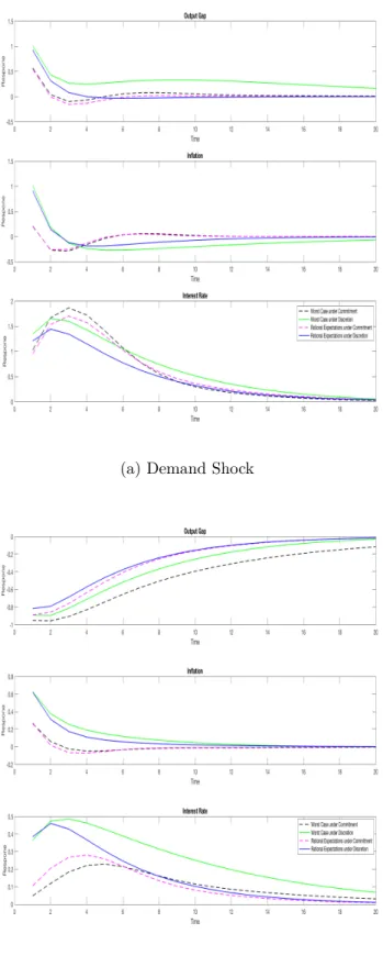
Under model uncertainty, when the economy faces a shock to aggregate demand, the monetary authority guards against model misspecification and formulates a more aggressive policy that would work well under the worst possible outcome of the shock. Central bank not only increases the nominal interest rate to a higher level compared to the case under rational expectations
4I restrict the extensions to add persistence in the IS and Phillips relations to keep the
but also keeps it that way for a longer time. Although the responses of output gap and inflation seem close with and without model uncertainty, it takes longer for inflation to go back to the steady state. Yet, as a response to a supply shock, the monetary authority takes a cautious stance.
When I allow for household utility to depend on both current consump-tion and on past consumpconsump-tion (as a reference level), the optimal consumpconsump-tion decision of the household takes into account not only the change in consump-tion but also the level of consumpconsump-tion, which ensures persistence in aggregate demand. Compared to the benchmark model, optimal response of the policy-maker under a demand shock is to raise the nominal rate substantially to keep the fluctuations in the out gap under control by allowing for a disinflation-ary process for the inflation rate. At the same time, when the source of the shock comes from the supply side, habit formation in consumption provides responses similar to the benchmark model.
I allow for indexation to past inflation by assuming that only some frac-tion of firms sets prices optimally whereas the remaining firms choose a price according to past inflation rate and the price set by both optimizing and non-optimizing firms in the previous period. Allowing for indexation to past infla-tion adds a backward-looking component into the Phillips Curve. A reasonable persistence in inflation leads the responses under a supply shock amplified for the nominal rate, inflation rate and the output gap.
While being intuitive, the study proposes some attracting findings on the optimal policy with a concern for robustness to model misspecification in New Keynesian models. First, the concerns about model uncertainty always make