T.C.
ISTANBUL AYDIN UNIVERSITY INSTITUTE OF GRADUATE STUDIES
NOVEL APPROACH IMMUNE TO PARTİAL SHADİNG FOR PHOTOVOLTAİC ENERGY HARVESTİNG FROM BUİLDİNG
INTEGRATED PV (BIPV) SOLAR ROOFS
MASTERS THESIS Farnaz Pourebrahimi
Department of Electrical & Electronic Engineering Electrical and Electronics Engineering Program
T.C.
ISTANBUL AYDIN UNIVERSITY INSTITUTE OF GRADUATE STUDIES
NOVEL APPROACH IMMUNE TO PARTİAL SHADİNG FOR PHOTOVOLTAİC ENERGY HARVESTİNG FROM BUİLDİNG
INTEGRATED PV (BIPV) SOLAR ROOFS
MASTERS THESIS Farnaz Pourebrahimi
(Y1713.300015)
Department of Electrical & Electronic Engineering Electrical and Electronics Engineering Program
Thesis Advisor: Prof. Dr Murtaza FARSADI
DECLARATION
I hereby declare with respect that the study “Novel Approach Immune to Partial Shading for Photovoltaic Energy Harvesting from Building Integrated PV (BIPV) Solar Roofs”, which I submitted as a Master thesis, is written without any assistance in violation of scientific ethics and traditions in all the processes from the Project phase to the conclusion of the thesis and that the works I have benefited are from those shown in the Bibliography. (.../.../20...)
FOREWORD
I would first like to thank my mother who was past away when she was alive she wanted me to be strong like her, her only aim was me and my sister be sucssesful in whole life. She got attempt for us to be knowledgeable persons .I owe alot to her. Also my sister Nazila Pourebrahimi and my uncle Hassan Dabbaghi who have always been supportive and encouraging, they raised me to become a good person and a positive member of society and were patient with me through good and better days and everthing i have accomplished is because of their effort and i hope i can make them happy in return for all they have done. I would like to thank Dr. Mitra Sarhangzade who helped me in my thesis who is really helpful and my real friend. Then i would like to thank my thesis advisor Prof. Dr. Murtaza Frasadi of Electric and Electronic Engineering department at Istanbul Aydin University. The door to Prof. Murtaza Frasadi’s office was always open whenever I ran into a trouble spot or had a question. I would like to thank all my teachers for having great influence on me, I would like also to thank department of Electric and Electronic Engineering and also Istanbul Aydin University and its library for providing me with access to all the books and articles that I needed to finish this work.
October, 2019 Farnaz Pourebrahimi
TABLE OF CONTENT
Page
FOREWORD ... iv
TABLE OF CONTENT ... v
ABBREVIATIONS ... vii
LIST OF FIGURES ... viii
LIST OF TABLES ... ix
ABSTRACT ... x
ÖZET ... xi
1. INTRODUCTION ... 1
1.1 Purpose of the Thesis ... 1
1.2 Solar Power System ... 1
1.3 Literature Review ... 2
1.4 Thesis Objective ... 5
1.5 Thesis Outline ... 5
2. PV CELLS, MODULE AND PV ARRAY ... 6
2.1 PV Modelling ... 7
2.2 Solar Irradiance ... 8
2.3 Solar Temperature ... 8
2.4 Boost Converter ... 9
3. LINEARIZATION ... 12
3.1 Steady state Equations ... 13
3.1.1 Relationship between the conversion function and the state space function ... 15
3.2 Nonlinear Control ... 15
3.2.1 Introduction ... 15
3.2.2 Feedback control ... 16
3.2.2.1 Input state linearization ... 17
3.2.2.2 Input-output Linearization ... 22
4. SIMULATION RESULTS ... 39
4.1 Introduction ... 39
4.2 Simulated Network ... 40
4.3 Steady-state analysis of DC-DC boost converter ... 40
4.4 linear controller of Boost Converter ... 43
4.4.1 Senario1 ... 44
4.4.2 Senario2 ... 45
4.4.3 Senario3 ... 48
4.4.4 Senario4 ... 49
4.5 Nonlinear controller of Boost Converter ... 52
4.6 GV curve ... 54
4.6.1 GV curve using linear controller ... 54
4.6.2 GV curve using nonlinear controller ... 56
REFERENCES ... 59 RESUME ... 60
ABBREVIATIONS
BIPV : Building Integrated PV CPG : Clean power generation DG : Distributed generation FC : Fuel cell
LTI : Linear time invariant MIMO: Multi-Input-Multi-Output MPPT : Maximum power point tracking PEC : Power electronic conversion PID : Proportional integral derivative PV : photovoltaic
PWM : Pulse with modulation SISO : Signal-Input-Signal-Output SP : Set point
LIST OF FIGURES
Page
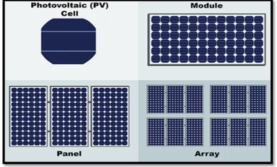
Figure 2.1: Photovoltaic cells, module, panels and arrays ... 6
Figure 2.2: Equivalent Circuit of the Solar Cell ... 7
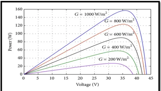
Figure 2.3: The plot of (P-V) in different irradiance ... 8
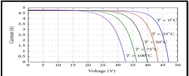
Figure 2.4: The plot of (V-I) in different temperature ... 9
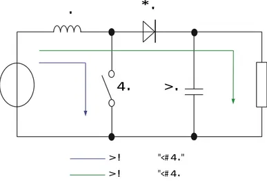
Figure 2.5: Boost Converter Simplified Schematic and Characteristics ... 10
Figure 3.1: Feedback path ... 28
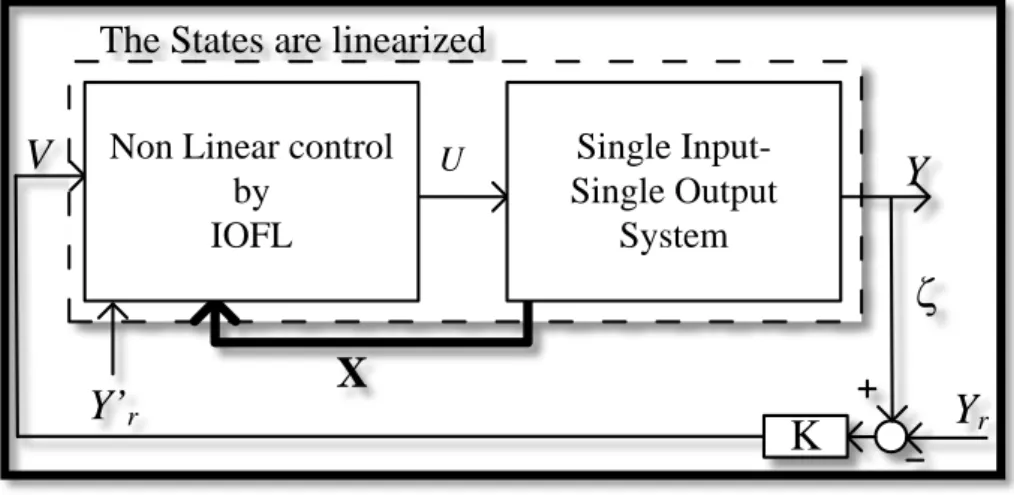
Figure 3.2: Shows how the input can be controlled to obtain the desired output by the input-output linearization ... 38
Figure 4.1: Simulated network topology ... 40
Figure 4.2: DC-DC boost converter topology ... 40
Figure 4.3: Intervals of DC-DC boost converter... 41
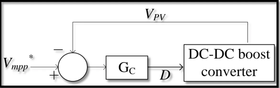
Figure 4.4: PI controller to have maximum voltage in input side of DC-DC boost converter ... 44
Figure 4.5: Simulation results of scenario 1- Linear controller ... 45
Figure 4.6: Simulation results of scenario 2- Linear controller ... 47
Figure 4.7: Simulation results of scenario 3-Linear controller ... 49
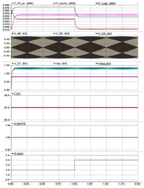
Figure 4.8: Simulation results of scenario 4- Linear controller ... 51
Figure 4.9: Nonlinear controller of DC-DC boost converter ... 53
Figure 4.10: Simulation results of scenario 4 - Nonlinear controller... 53
Figure 4.11: Vmpp changes with irradiance changes ... 54
Figure 4.12: Vmpp changes with irradiance changes for fix load and temprature -Linear controller ... 55
Figure 4.13: Vmpp change with irradiance changes-Linear controller ... 55
Figure 4.14: Vmpp changes with irradiance changes for fix load and temprature -NonLinear controller ... 56
LIST OF TABLES
Page Table 4.1: Solar Panel Specification ... 44
NOVEL APPROACH IMMUNE TO PARTIAL SHADING FOR PHOTOVOLTAIC ENERGY HARVESTING FROM BUILDING
INTEGRATED PV (BIPV) SOLAR ROOFS ABSTRACT
In recent years, much attention has been paid to the use of multi-megawatt photovoltaic
systems in power distribution and over-distribution systems. Also, due to lower costs of photovoltaic systems, grid-connected photovoltaic technology has improved significantly. However, the increasing growth of photovoltaic systems may have adverse consequences for power systems in terms of harmonics, voltage profiles, stability, and so on. Therefore, this dissertation offers the best possible integration of photovoltaic generators into a grid-connected DG converter with multiple photovoltaic panel inputs. The challenging issues in designing, and analysing such systems arise from the complex dynamic model of these systems, which is rooted in nonlinear characteristics of voltage and current in solar modules. In this thesis, a step-by-step process of modelling, designing, and analysing various parts of the system such as: photovoltaic array, DC bus capacitor, voltage source inverter, passive output filters and inverter current controller and DC bus voltage is presented. Also in this thesis a new method for designing DC bus voltage controller based on nonlinear voltage-current characteristic linearization of photovoltaic module is presented and a criterion based on the maximum power sequential controller parameters to improve the performance of this controller is extracted under changes in radiation level. Has been. The results show the satisfactory performance of the whole system and the designed controllers as well as the accuracy of the analytical criteria extracted for the stable operation of the system under various operating conditions.
Keywords: Photovoltaic Systems, MPPT Maximum Power Point Tracking, Boost Converter
BİNA ENTEGRE PV (BIPV) GÜNEŞ ÇATILARINDAN FOTOVOLTAİK ENERJİ HASADI İÇİN KISMİ GÖLGELEMEYE BAĞIŞIKLIK YENİ
YAKLAŞIM ÖZET
Son yıllarda güç dağıtımında ve aşırı dağıtım sistemlerinde çok megawatt fotovoltaik sistemlerin kullanımına çok dikkat edilmiştir. Ayrıca, fotovoltaik sistemlerin düşük maliyetleri nedeniyle, şebekeye bağlı fotovoltaik teknolojisi önemli ölçüde iyileşmiştir. Bununla birlikte, fotovoltaik sistemlerin artan büyümesi, harmonikler, voltaj profilleri, kararlılık ve benzeri açıdan güç sistemleri için olumsuz sonuçlara yol açabilir. Bu nedenle, bu tez, fotovoltaik jeneratörlerin çoklu fotovoltaik panel girişlerine sahip bir şebekeye bağlı DG dönüştürücüsüne mümkün olan en iyi entegrasyonunu sunar. Bu tür sistemlerin tasarlanması, analiz edilmesi ve analiz edilmesindeki zorlu konular, güneş modüllerindeki gerilim ve akımın doğrusal olmayan özelliklerinden kaynaklanan bu sistemlerin karmaşık dinamik modelinden kaynaklanmaktadır. Bu tezde sistemin fotovoltaik dizisi, DC bara kondansatörü, gerilim kaynağı invertörü, pasif çıkış filtreleri ve DC invertör akım ve gerilim kontrolörleri gibi çeşitli parçalarını modelleme, tasarlama ve analiz etme aşamalı bir süreci sunulmaktadır. Ayrıca bu tezde, fotovoltaik modülün doğrusal olmayan voltaj-akım karakteristik doğrusallaştırmasına dayalı DC bara voltaj kontrolörü tasarlamaya yönelik yeni bir yöntem sunulmakta ve radyasyon seviyesindeki değişiklikler altında bu kontrolörün performansını arttırmak için maksimum güç sıralı kontrolör parametrelerine dayanan bir kriter çıkarılmaktadır. Oldu. Sonuçlar, tüm sistemin ve tasarlanan kontrolörlerin tatmin edici performansını ve çeşitli çalışma koşulları altında sistemin kararlı çalışması için çıkarılan analitik kriterlerin doğruluğunu gösterir.
Anahtar Kelimeler: Fotovoltaik Sistemler, MPPT Maksimum Güç Noktası İzleme, Boost Dönüştürücü
1. INTRODUCTION
1.1 Purpose of the Thesis
A phenomenon that generates sunlight without the use of electrically driven mechanisms is called a photovoltaic phenomenon, and any system that uses this phenomenon is called a photovoltaic system. In this method, the energy of the sun's radiation is converted into electrical energy without any intermediary and only with the help of photovoltaic cells. The main basis of this phenomenon is based on the photoelectric effect. Light energy causes electrons to be separated from matter and this effect is the basis of the work of photovoltaic cells.
The duties considered in this dissertation are:
1. How to Maximize the Power of a Solar Panel Strand the conventional MPPT methods are investigated taking into account the temperature changes and the intensity of radiation in the environment on the solar panel.
2. How to integrate the maximum power obtained from several independent solar panels.
3. A structure based on power electronic devices such as DC-DC converter structures is designed to simultaneously interconnect multiple independent solar panels to integrate their output power.
4. Proposed the investigation of the PV technology implementation of the building integrated photovoltaic (BIPV). The study will tell the grid integration of the photovoltaic strings composed of the BIPV modules. Two strategies are compared PWM (Pulse Width Modulation) and non-linear controller.
1.2 Solar Power System
Sun powered vitality, in its most straightforward structure, is vitality which is produced by the sun. This sun energy is caught and afterward transformed into usable power. This power can be utilized in your home, work environment, or
practically whatever other territory where electrical force is required. The world's sun resembles an atomic reactor which discharges little vitality bundles called photons. These photons head out 150 million km to the world's surface.
1.3 Literature Review
The Sun is the source of the various energies that exist in nature. Simple technology, non-polluting air and the environment, and most importantly the storage of fossil fuels for future generations or converting them into valuable materials and artefacts using petrochemical techniques, are the main reasons why our country needs to use solar energy. As well as the increasing population of the world, the limitation of energy resources and the environmental impacts of the fossil fuel exterior consumption, the world's attention has been drawn to the use of renewable energies. In this project, while introducing photovoltaic systems connected to the grid as a new energy system, the optimal conditions for the installation of these cells have been investigated. Since the efficiency of the cells is low and their initial cost is somewhat high, they must be exploited in a way that always works at their maximum power point, thereby maximizing efficiency and making the system more efficient. Given that in most applications they use photovoltaic modules as scattered generation sources and utilize other techniques to utilize solar energy in mass production, the importance of studying this electricity generation system is important. Therefore, using these small power plants connected to the distribution grid, effective steps can be taken in terms of grid safety and energy loss reduction. The target set by the European commission for the energy budget from the renewables by the end of the year 2020 is 20% [1]. By this a contribution can be done in the global warming and the greenhouse effect can be stabilized. The solar energy source is the best and clean among all world power productions [2].
Today, with the advances in industry and technology, energy supply has become a major issue. Common sources of fossil energy production to which are mostly non-renewable, this issue for communities due to the release of harmful pollutants into the environment. According to research by scientists, these resources are running out by the end of the 21st century. Photovoltaic system is
one of the best ways to use renewable sources such as solar energy. The most important limiting factor for solar energy use is the issue of high cost of electricity produced, low efficiency, limited capacity to operate at full capacity throughout the day, - high installation space, energy storage using batteries Expensive as well as low solar energy density and complexity of construction method can be reduced by choosing the right methods and structures. It should be noted that the development of this technology in recent years has increased the accuracy of predicting the cost of using photovoltaic systems and will provide the parameters involved in order to obtain the maximum power. In recent years, solar energy and photovoltaic systems have become more popular as a source of green energy, due to the ease of installation, the lack of greenhouse gases and their relatively long lifespan (approximately 25 years). The discovery of the photovoltaic phenomenon is attributed to the French physicist Alexandre Edmond Becquerel, who observed in Year 1839 that the voltage of the battery increased when its silver plates were exposed to sunlight. He observed this phenomenon from childhood as a scientist's father as a student and then research assistant at the age of 19. His father Antoine César Becquerel (1788-1878) discovered the piezoelectric effect. This work was first studied on solids such as selenium by Heinrich Hertz in 1870. But it was the first report of a PV phenomenon in a solid that year; two Cambridge scientists, R.E. Day and W.G. Adams explained in an article to the Royal Society the changes in the electrical properties of selenium when exposed to light. In 1883 Charles Edgar Frits, a New York-based electrical engineer, built a selenium cell that was in some ways similar to modern silicon solar cells. The cell consisted of a thin selenium wafer that was covered with a theory of thin gold foils and a protective sheet of glass. But the cellulose he made was very low yield. Less than 1% of the solar energy emitted to the surface of this elementary cell was converted to electricity. However, selenium cells were eventually widely used in photographic photometers. In 1887, Heinrich Hertz discovered that ultraviolet light changes the minimum voltage needed to generate a spark to jump between two metal electrodes. In 1904 Hallwachs discovered that it is a combination of copper and light-sensitive copper oxide. Also this year Einstein published his paper on the photoelectric effect. In 1916, The photoelectric effect was proved
by the experimental results of Millikan. In 1918, Polish scientist Czochralski proposed a way to grow single crystalline silicon. In 1923, Einstein won the Nobel Prize for his work in explaining the photoelectric effect. In 1951, a single crystalline cell from germanium was grown as a p - n bond. In 1954, The photovoltaic effect on cadmium was reported. The initial work was done by Rappaport, Loferski and Jenny. Researchers Daryl Chapin, Gerald Pearson and Calvin Fuller reported a 4.5% efficiency silicon solar cell lab, which reached 6% within a few months of working with a research team. They sent their results to the Journal of Applied Physics.
In 1958, Hoffman Electronics reached 9% efficiency cells .In 1960, Hoffman Electronics reached 14% efficiency cells. In 1961, The first conference of PV specialists was held in Washington. In 1964, The Nimbus spacecraft was launched with a 470-W solar cell array. In 1968, The OVI-13 satellite launched with two CdS panels. In 1984, The IEEE Morris N. Liebmann Award was presented to David Carlson and Christopher Wronski at the 17th Conference of Photovoltaic Specialists for their decisive efforts to use amorphous silicon in high-cost solar cells. In 2000, a family in Colorado set up a 12-kilowatt solar electric system on their home.
In interconnected systems of electricity, with regarding economies of scale, the generation of electricity is centrally carried out by large power plants. [3]
PV systems are one of the unique technologies that are accessible for the well-organized use of solar power. In coming ages the possibility for PV applications, the four factors should be considered on top, that are cost reduction, efficiency, building integrated photovoltaic (BIPV) applications, BIPV storage system. The better performance of BIPV can get by using advance techniques in construction to merge with BIPV technology. The BIPV technology has the protection phenomenon from , weather, thermal and noise etc. BIPV semi-transparent installation permits light. PV systems are popular nowaday because there is no need for the ground space and too many unused roof tops are available. The installation cost is also decreased by using BIPV technology. The cost is decreased because the BIPV have no bracket and rails. Some factors should be taken into account to get maximum outcome from the
system like, temperature, partial shadowing, installation angle and the direction [4].
The number of consumers are increasing every year for BIPV technology, due to this reason the architectures and manufacturers are using new methods to create new products as per the market requirements. SANYO, SCHOTT SOLAR, SHARP AND SUN-TECH are working on new BIPV products for facades, skylights and windows. BIPV is already accepted in Europe in coming years the rest of the world will accept this technology [4].
1.4 Thesis Objective
The objective of this thesis is injecting of PV modules in MPP point to enhance the maximum power of PV modules. In the thesis, DC-DC converter is used for MPPT while linear and nonlinear controller to control the converter for achieving maximum power of PV modules.
1.5 Thesis Outline
The second chapter is about the components that are used in the circuit simulation, why they are used and their use.
The third chapter talks about our proposed circuit simulation in the PSCAD Simulink environment. Results are discussed and compared for different technologies that we used, in detail in the fourth chapter. At the end the fifth chapter is about the conclusion and future expectations.
2. PV CELLS, MODULE AND PV ARRAY
Solar energy is converted to electricity through solar cells, but the energy produced by this cell is scarce, so to generate more energy, solar cells are connected in series in photovoltaic modules. Form, which is capable of producing a great deal of electrical power.
A PV cell alone generates a voltage of about 0.5 volts, which is a small amount. A module is created to generate larger voltages by series of several cells. A voltage of 12 or 24 volts is common for modules, which is obtained by sequencing 36 or 72 cells, respectively. Figure (2-1) shows the characteristic of a module consisting of 36 cells. The amount of current produced by the PV module also depends on the area of the solar cells. A larger area for each solar cell produces a higher current. If more output power is needed, the modules must be connected in series or in parallel, which will result in an array. Figure (2-1) schematically shows a cell, modulus and PV array. Panels for grid-connected photovoltaic systems are very limited, and in order to supply voltage and current in larger sizes, the solar cell composition must be series and parallel
A solar panel or module can be assembled into a series of solar cells to allow the desired voltage and current. For achieving high voltage, we need to do series all the cells, and also be able to reach more current, we need to connect all solar cells in parallel.[5]
2.1 PV Modelling
An ideal solar cell works as a currents source, and that current causes from the light of the sun falling on the cell known as intensity. There are some components needed to develop equivalent model of solar cell and loss are represented by adding a diode in parallel but in reverse direction. In simple model the only one diode added in solar cell equivalent circuit. In general, the (I-V) curve of the diode includes temperature effect. The other losses occurs due to series and parallel (shunt) resistance that are represents by Rs and Rp .The series resistance is the resistance of the solar cell, and Rp is the leakage path of the current in the solar cell, that’s why it comes always in parallel with current source. The Equivalent circuit of a solar cell is shown in figure 2.2.[5]
Figure 2.2: Equivalent Circuit of the Solar Cell The I-V equation is given by
The I-V equation of a simple solar cell model will be given below
2.2 Solar Irradiance
Irradiance is one of effective way for changing output of power in solar panel. The relation of decreasing or increasing of power with irradiation is directly. However, solar irradiance is available during day then declines till sunset so that the result of power output is fluctuated during day.
Figure 2.3: The plot of (P-V) in different irradiance
2.3 Solar Temperature
The output of power in solar panel depends on the modules temperature which are working. First of all, the temperature of module is higher than environment so this temperature can be changed by effects of irradiance, wind, etc. In the noon when the temperature of module is about 55,60 degrees the ambient
( 1.2)
(
)
1 Re IPH ISC K TC T f λ = + − (1.3)temperature is about up to 20 degrees. The higher temperature of module which traps the radiation and enhance the module temperature
Tmod=Tamb+Kpin
Tamb=ambient temperature Pin=radiation temperature K= constant (0.02 and 0.03)
With increasing cell temperature, the current of short circuit increases in fact in open circuit voltage declines. Decrease in Voc is more common than the increase in Isc .As a result, the power output and efficiency of solar cells and modules step down.
Figure 2.4: The plot of (V-I) in different temperature 2.4 Boost Converter
Step-up or boost converter converts a low level input voltage into a higher output voltage. A simplified circuit diagram and the main current and voltage waveforms are shown in Figure (2.5)
VOUT=VIN /1-σ Valid when VIN<VOUT (2-1)
Figure 2.5: Boost Converter Simplified Schematic and Characteristics
When S1 closed, current flows through the inductor L1 that increases linearly. During this period the load current is supplied in capacitor C1. When the switch is opened again, the stored energy in the inductor causes high output voltage superimposed onto the input voltage. The resulting current flows via the
freewheeling diode D1 to supply the load and also recharge C1. The current through the inductor falls linearly and proportionally to (VOUT - VIN)/L1. [6] The derivation of the transfer function is similar to that in the previous section, only the basic equations are rearranged:
For the ON condition:EnergyIN = VIN tON
3. LINEARIZATION
In this section we deal with dynamical systems, which can be described with a few ordinary first order differential equations in Equation 3-2, in which the state variables represent the dynamics of the system's memory relative to its past. Equation 3-6 in nonlinear control represents the next output vector that contains variables that we are interested in studying in dynamic system analysis, such as variables that can be physically measured or variables that are required have to behave in a certain way.
In this chapter, we will present some of the feedback systems analysis tools that are displayed by feedback. Our interest in feedback systems is due to two aspects: First, many physical systems can be represented by feedback. From the point of view of control engineers, this is quite obvious, since feedback plays a key role in automated control systems. These systems are used to measure, process and feedback specific variables to find control inputs. Of course, the importance of feedback systems is not just limited to control systems, because many systems that are not initially modeled as control systems can be represented in such a way as to take advantage of system-specific tools. To gain control. [7]
The second aspect of the importance of feedback systems is that the feedback structure opens a new field for scientific challenges and solutions. Therefore, for many years, the analysis of the feedback system has been the subject of hot research. In this chapter we discuss the design of feedback control and introduce nonlinear control design based on I / O linearization.
There are many controls that require the use of feedback control. In addition, there are various formulations for control issues depending on the purpose of the design. Various things like stabilization, tracking, and so on can cause a variety of issues in control. In each of these problems, we are faced with either a form of state feedback that can measure all the state variables or an output feedback mode where only the output vector can be measured. It is typically
smaller than the state vector dimension. In this section we begin our review with the stabilization problem in both case feedback and output feedback. [7]
3.1 Steady state Equations
In state space analysis, we deal with three types of variables that are involved in modeling the dynamic behavior of the system: input variables, output variables, and state variables. Suppose a multi-input/ outputs system has n integrator and has r inputs: u1(t),u2(t),...,ur(t) and m outputs: y1(t),y2(t),...,ym(t). We define the n outputs of integrators as state variables
So the system can be defined as:
And the system outputs are as follows:
) ( ),..., ( 2 ), ( 1 t x t xr t x (3-1) (3-2) ,..., 2 , 1 ; ,..., 2 , 1 ( ) ( ' . . . ,..., 2 , 1 ; ,..., 2 , 1 ( 2 ) ( ' 2 ; ,..., 2 , 1 ; ,..., 2 , 1 ( 1 ) ( ' 1 r u u u n x x x n f t n x r u u u n x x x f t x t r u u u n x x x f t x = = = (3-3) ,..., 2 , 1 ; ,..., 2 , 1 ( ) ( . . . ,..., 2 , 1 ; ,..., 2 , 1 ( 2 ) ( 2 ; ,..., 2 , 1 ; ,..., 2 , 1 ( 1 ) ( 1 r u u u n x x x n h t m y r u u u n x x x h t y t r u u u n x x x h t y = = =
Defining the equation (3-4):
Equations 3-2 and 3-3 can be written as follows:
Equation 3-5 is the state equation and equation 3-6 is the output equation. If the f and h functions include t, the system is time-varying. By linearizing the equations 3-5 and 3-6 around the work point, the state equation and the linearized output equation are obtained:
Where A(t) is the state matrix, B(t) is the input matrix, A(t) is the output matrix and D(t) is the direct transfer matrix. If time is not explicitly included in the h and f functions, the linear system is time independent. The equations 5 and 3-6 are then simplified as follows:
In which the state matrix, input matrix, output matrix, and direct transfer matrix are read. Unless explicitly included in functions and time, the linear system is independent of time. Then the equations 3-5 and 3-6 are simplified as follows:
(3-9) (3-10) ) , , ( ) ( ) , , ( ) ( ' t u x h t y t u x f t x = = ) ( ) ( ) ( ) ( ) ( ) ( ) ( ) ( ) ( ) ( ' t u t D t x t C t y t u t B t x t A t x + = + = ) ( ) ( ) ( ) ( ) ( ) ( ' t Du t Cx t y t Bu t Ax t x + = + = = = = ) ( . . . ) ( 2 ) ( 1 ) ( , . . . 2 1 , ) ( . . . ) ( 2 ) ( 1 ) ( , . . . 2 1 ) , , ( t m u t u t u t u n h h h t m y t y t y t y n f f f t u x f (3-4) (3-5) (3-6) (3-7) (3-8)
Equations 3-9 and 3-10, respectively, are the state equation and the output equation of a time-independent linear system.
3.1.1 Relationship between the conversion function and the state space function The one-input-one-system conversion function can be obtained from its state equations. We have a system with the following conversion function:
) ( ) ( ) ( s U s Y s G = (3-11)
This system can be described in the state space with the following equations:
Du Cx y Bu Ax x + = + = ' (3-12) (3-13) Where x is the state vector, u is the input and y is the output. Outputs and inputs in the Laplace domain are obtained as follows:
(3-14) (3-15) And the conversion function is equal to:
(3-16)
So the equation of the G(s) attribute is |SI-A| In other words, the eigenvalues of A and G(s) poles.[7]
3.2 Nonlinear Control 3.2.1 Introduction
When engineers analyze and design nonlinear dynamic systems in electrical circuits, mechanical systems, control systems, and other engineering applications, it is necessary to obtain and utilize a wide range of tools and tools in nonlinear analysis. Use them. In this chapter, we introduce one of these tools, called Feedback Linearization. In this section we deal with dynamic systems
) ( ] 1 ) ( [ ) ( ) ( 1 ) ( ) ( s U D B A sI C s Y s BU A sI s X + − − = − − = A sI s Q D B A sI C s G − = + − − = ( ) 1 ( ) ) (
that can be described with a few ordinary first-order differential equations in Equation 2-3, in which the state variables represent the dynamics of the system's memory relative to its past. Equation 3-6 in nonlinear control represents the next output m vector, which contains variables that we are interested in studying in dynamic system analysis, such as variables that can be physically measured or variables that are required Have to behave in a certain way.[8]
3.2.2 Feedback control
In this chapter, we will present some of the feedback systems analysis tools that are displayed by feedback. Our interest in feedback systems is due to two aspects: First, many physical systems can be represented by feedback. From the point of view of control engineers, this is quite obvious, since feedback plays a key role in automated control systems. These systems are used to measure, process and feedback specific variables to find control inputs. There are many controls that require the use of feedback control. In addition, depending on the purpose of the design, there are various formulations for control problems. Various things like stabilization, tracking, and so on can cause a variety of issues in control. In each of these problems, we are faced with either a form of state feedback that can measure all the state variables or an output feedback mode where only the output vector can be measured. It is typically smaller than the state vector dimension. In this section we begin our review with the stabilization problem in both case feedback and output feedback.[8]
The problem of state feedback stabilization for the ( ) ( , , )
' t f x u t
x =
system is to design the
u
=
γ
( t
x
,
)
feedback control rule so that the origin of x=0 is a uniform asymptotic stable equilibrium point for the following closed loop system:(3-17)
If we know how to solve this problem, we can stabilize the system with any optional P point. Because you can move p, y=x-p to the source by changing the
)
,
( t
x
u
=
γ
variable. The rule of thumb is usually called the static x state)) , ( , , ( ) ( ' t f x t xt x =
γ
because it is a memory-free function. Sometimes we use the following dynamic feedback control rule:
(3-18) The dynamic response and its input are x:
In this chapter we consider a set of nonlinear systems as follows:
And we convert this system to a linear equation system by controlling the
v
x
x
u
=
α
(
)
+
β
(
)
state feedback and changing theZ
=
T
(x
)
variable. To thisend, we first introduce the concept of state input linearization in which the equation of state is linearized and then examine the input-output linearization where emphasis is placed on from u - y input-output mapping linearization 3.2.2.1 Input state linearization
Definition: The following nonlinear system:
Where f :Dx →Rn, and p n R x D
g: → × are smooth enough (all of its partial
derivatives are defined and continuous), over the
n R x
D ⊂ domain, the inline
linearity - say, if the dependencies mapping (the mapping itself and the inverse mapping) - derivative. Acceptable) T :Dx →Rnexist if Dz =T( xD ) contains the origin and modify the
z
=
T
(x
)
variable of system 21-23:)
,
,
(
x
t
z
u
=
γ
)
,
,
(
'
g
x
t
z
z
=
(3-19)u
x
g
x
f
x
'
=
(
)
+
(
)
, Y =h(x) (3-20)u
x
g
x
f
x
'
=
(
)
+
(
)
(3-21)(
)[
(
1
'
Az
B
x
u
x
z
=
+
β
−
−
α
(3-22)Where (A,B) is controllable and, β(x) for all
x
∈
D
x
values, is non-singular. bychoosing:
The equations (3-22) can be written as (3-24):
Usually α and β are expressed in terms of x coordinates because feedback control is built into this coordinate machine. Now consider the Input Linear System - Equation Mode 21-23 and assume
z
=
T
(x
)
is a variable change that makes the system in form 22-23. Then we have:On the other hand, from equation (3-23) we can write:
It follows from Equations 3-25 and 3-26 that we must draw:
For all values of x and u be in the territory in question.
First, by selecting u=0 we convert this expression into two equations:
Therefore, it can be concluded that any T(.) function that converts Equation 21-23 to Equation 22-21-23 must apply to the partial differential equations 28 and 3-29. Conversely, if the T(.) mapping is such that the relationships 3-28 and 3-29
)) ( 1 ( ) ( 0 )), ( 1 ( ) ( 0 z =
α
T− zβ
z =β
T− zα
)] ( )[ ( 1 ) ( )] ( )[ ( 1 ' Az B x u x AT x B x u x z= + β− −α = + β− −α )] ( )[ ( 1 ) ( ] ) ( ) ( [f x G x u AT x B x u x x T + = +β
− −α
∂ ∂ ) ( 1 ) ( ) ( ) ( 1 ) ( ) ( x B x G x T x x B x AT x f x T − = ∂ ∂ − − = ∂ ∂ β α β (3-23))]
(
0
)[
(
1
0
'
Az
B
x
u
x
z
=
+
β
−
−
α
(3-24))
(
)
(
[
'
'
f
x
G
x
x
T
x
x
T
z
=
∂
∂
=
∂
∂
+
(3-25) (3-26) (3-27) (3-28) (3-29)are for α,β, A,B and with certain properties, then it can be easily shown that changing the variable z=T(x) equation 21-23 to 3 -22 Converts. Therefore, the existence of α,β,A,B values, and which apply to the prtial differential equations 3-28 and 29-29, is a necessary and sufficient condition f If a nonlinear system is an input-state linearity, the z=T(x) mapping that renders the system in Figure 22-2 is not unique. The simplest way to get this is to point out that by applying the linear transformation of
ξ
=Mz (which M is non-singular) to Equation 22-2, the state equation inξ
coordinates will be as follows: or the linear 21-23 input-state system.[9]Which is still in Equation 22-2. But the matrices are different in
that. Therefore, the combination of z=T(x) transformers results in a new conversion that converts the system into a specific 22-23 structure. Given the uniqueness of the T , the equations of 28-23 and 29-23 can be simplified. We focus on single-input systems. The g matrix then becomes a (A,B) column vector, and for any g controllable pair it can be found that the KK matrix can be focalized to (A,B) That is:
where in: The term MT(x) T C B T C B λ ξ = λ
can be considered within the sentence ) ( ) ( 1 x x C B β− α
T therefore, without reducing the generality of the subject, it )] ( )[ ( 1 1 ) ( ' x MAM ξ MBβ x u α x ξ = − + − − C B MB T C B C A MAM−1= + λ , =
1
1
.
.
.
0
0
0
,
0
0
0
0
0
0
0
1
0
0
0
0
0
0
0
.
0
.
0
.
0
.
.
.
1
0
0
0
.
.
.
0
1
0
×
=
×
=
n
C
B
n
n
C
A
(3-30) (3-31) (3-32)can be assumed that A and B matrices in Equations 28-23 and 29-23 are focal Ac and Bc matrices. Suppose we have:
It can be easily researched:
Which are α and β are numerical functions. Using these equations in Equations 28-23 and 29-23, the partial differential equations are simplified and the equation 28-23 can be written as follows:
1 ) ( . . . ) ( 3 ) ( 2 ) ( 1 ) ( × = n x n T x T x T x T x T (3-33)
=
−
×
−
=
−
−
)
(
1
0
.
.
.
0
)
(
1
,
1
)
(
)
(
)
(
.
.
.
)
(
2
)
(
)
(
1
)
(
x
x
C
B
n
x
x
x
n
T
x
T
x
x
C
B
x
T
C
A
β
β
β
α
α
β
(3-34) ) ( ) ( ) ( ) ( ) ( 1 . . . ) ( 2 ) ( 1 x x x f x n T x n T x f x n T x T x f x Tβ
α
− = ∂ ∂ = ∂− ∂ = ∂ ∂ (3-35)Also, Equation 29-23 can be simplified to
It is therefore T1(x)necessary to find the function that applies to the following relationships:
That:
If the T1(x) function can be found to satisfy Equation 3-37, then α and β will be equal to:
0
)
(
1
)
(
0
)
(
1
.
.
.
0
)
(
1
≠
=
∂
∂
=
∂
−
∂
=
∂
∂
x
x
g
x
n
T
x
g
x
n
T
x
g
x
T
β
(3-36) 0 ) ( ; 1 ,..., 2 , 1 , 0 ) ( = = − ∂∂ ≠ ∂ ∂ x g x n T n i x g x i T (3-37)1
,...,
2
,
1
),
(
)
(
1
∂
=
−
∂
=
+
x
f
x
i
n
i
T
x
i
T
(3-38))
(
)
(
)
(
)
(
1
)
(
x
g
x
n
T
x
f
x
n
T
x
x
g
x
n
T
x
∂
∂
∂
∂
−
=
∂
∂
=
α
β
(3-39) (3-40)Therefore, the problem in question has been solved by solving T1 Equation (37-37) to find a reduction. In linearization, we stabilize the system relative to the
equilibrium point of the open ring x* that is,
f
(
x
*
)
=
0
. For this purpose, we select the T mapping so that the x* point is mapped to the source, T(x*)=0 This can be done by solving Equation 3-37 and finding T1 by condition of)
0
*
(
x
=
T
[9]
3.2.2.2 Input-output Linearization
When specific output variables are considered, such as tracking control problems, the state model is expressed in terms of state and output equations. In this case, the previous method of linearizing the state equation does not necessarily lead to linearization of the output equation. For example, if the
system:
Includes output y=x2, variable change and feedback control rule as follows:
Concludes: u x x x a x + − = = 2 1 ' 2 2 sin ' 1 (3-41) v x a x u x a z x z 2 cos 1 2 1 2 sin 2 1 1 + = = = ) 2 ( 1 sin 2 ' 2 1 ' a z y v z z z − = = = (3-42) (3-43)
Here, although the state equations are linear, because of the nonlinearity in the output equation, solving the problem of trace control will be complicated. Considering both the state and output equations in the coordinates, it can be
seen that using the state feedback control lawu= 2x1 +v, the linear model is expressed as follows:
Now we can solve the problem of trace control with the help of linear control theory. This argument shows that sometimes it is better to obtain linearized input-output mapping, even though part of the state equation remains nonlinear. This point is the basis of the I / O linearization problem discussed in this section. One of the important points in I / O linearization is that I / O linear mapping may not be applicable to all system dynamics. As an example in the above example, the complete system is described by the following equation:
It is observed that the state variable x1 has nothing to do with the output of y, in other words, the linear feedback control has made the x1 variable invisible from the y perspective. When designing a trace, then, you need to make sure the x1 variable is stable. Because the simple control law, based on the input-output linear mapping, may lead to the ever-increasing x1(t) signal. Consider the following single-input system:
That, f,g,h in the realm of
D
⊂
R
n
are smooth enough. The simplest mode of input-output linearization occurs when the system is both linear-input linear and input-output linearized. We first assume the system to be linear-input linear,2 2 ' x y v x == ) ( ) ( ) ( ' x h y u x g x f x = + = 2 ' 2 2 sin ' 1 x y v x x a x = = = (3-44) (3-45) (3-46)
considering T1(x)as one of the solutions to Equation 3-37. In addition, we assume that the output function h(x) is equal to T1(x) Then, by changing the z=T(x) variable and
u
=
α
(
x
)
+
β
(
x
)
v
state feedback control, we get to system 3-47:That (Ac,Bc,Cc) is the focal point of the chains of n integrator. That is, Ac and Bc is in the form of Equation 3-32, and for Cc we also have:
: n this system, both state and output equations are linear. If the output function h(x) is known, it can be directly investigated whether it is true in condition 3-37 and no longer need to solve the partial differential equations. Condition 3-37 can be interpreted as a constraint on the dependence of y derivatives on
)
(
)
(
1
x
=
h
x
ψ
The derivative function y’ equals:
If so, then: z C C y v C B z C A z = + = '
[
]
n C C = 1 0 . . . 01× ] ) ( ) ( [ 1 , f x g x u x y + ∂ ∂ =ψ
(3-47) (3-48)0
)
(
1
=
∂
∂
x
g
x
ψ
)
(
2
)
(
1
,
f
x
x
x
y
ψ
=
ψ
∂
∂
=
(3-49) (3-50) ] ) ( ) ( [ 2 ) 2 ( f x g x u x y + ∂ ∂ =ψ
(3-51)If so, we have:
Repeating this process results if
h
(
x
)
=
ψ
1
(
x
)
Apply to Equation 3-37, namely:That:
Then
u
In the equationsy
n
−
1
,...,
y
'
,
y
Does not appear and is only present in the equation with a non-zero factor:This equation shows that the linear system is input-output because the following feedback control rule:
) ( 3 ) ( 2 ) 2 ( x x f x y =∂
ψ
∂ =ψ
] ) ( [ ) ( 1 v x f x n x g x n u + ∂ ∂ − ∂ ∂ =ψ
ψ
0 ) ( 2 = ∂ ∂ x g x ψ (3-52) 0 ) ( ; 1 ,..., 2 , 1 , 0 ) ( = = − ∂∂ ≠ ∂ ∂ x g xn n i x g xi ψ ψ ,..., 2 , 1 ), ( ) ( 1 ∂ = ∂ = + x f x i i x i ψ ψ x g x n x f x n n y( ) ( ) ( ∂ ∂ + ∂ ∂ =ψ
ψ
(3-53) (3-54) (3-55) (3-56)Input-output mapping as a formy(n) =v Reduces to a chain of integrators. If
in the equation of a derivativey(n 1),...,y'(t)
+
It appears that you can linearize the input-output mapping again. Specifically if
h
=
ψ
1
(
x
)
Apply the values of the equation in the following equation:Then we will have:
And the Passover Control Act 3-59:
Input-Output Mapping as Chains of Integratorsy(r) =v In this case, the integer is defined as the relative degree of the system according to the following definition: The nonlinear system of Equation 3-46, provided that the functions onh:D→R and f :D→Rn g:D→ Rnon the domain
D
⊂
R
n
are sufficiently smooth, have a relative degree( 1≤r≤n) the area D0⊂ Dif we have all values of:
That : 0 ) ( ; 1 ,..., 2 , 1 , 0 ) ( ≠ ∂ ∂ − = = ∂ ∂ x g x r r i x g x i
ψ
ψ
u x g x r x f x r r y( ) =∂∂ψ
( )+∂∂ψ
( ) R D h: →0
)
(
;
1
,...,
2
,
1
,
0
)
(
=
=
−
∂
∂
≠
∂
∂
x
g
x
r
r
i
x
g
x
i
ψ
ψ
1
,...,
2
,
1
),
(
)
(
1
),
(
)
(
1
∂
=
−
∂
=
+
=
f
x
i
r
x
i
x
i
x
h
x
ψ
ψ
ψ
(3-57) (3-58) (3-59) (3-60) (3-61) ] ) ( [ ) ( 1 v x f x r x g x r u + ∂ ∂ − ∂ ∂ =ψ
ψ
If the relative degree of the system is equal r, then the linearity of the input-output system is linear and if it has a relative degree then both the input-state linearity and the input-output linearity are n. To further investigate the control of input-output linear systems and concepts related to internal stability, we further analyze the linear system with the conversion function H(s):
That
deg
D
=
n
anddeg
N
=
m
<
n
And the relative degree is equal tom n
r= − It can be done by Euclidean division D(S) is shown:
That Q(s) and R(s) Which are respectively, polynomials outside and remaining. According to Euclidian Which are, respectively, polynomials outside and remaining.
The first coefficient Q(s) is equal with bm
1
, According to this show we can write H(s) in this way:
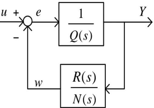
Therefore, we can write H(s) as a reason of a negative feedback system that
) ( 1 s
Q On the way forward and
(
)
)
(
s
N
s
R
there is a feedback path (Figure (3-1)).
0
...
1
1
0
...
1
1
)
(
)
(
)
(
a
n
s
n
a
n
s
b
m
s
m
b
m
s
m
b
s
D
s
N
s
H
+
+
−
−
+
+
+
−
−
+
=
=
) ( ) ( ) ( ) (s Q s N s R s D = + m b k n s m b n k n s m b s Q( )= 1 + −1 −1+...+ 0 m R r m n Q= − = , deg < deg ) ( ) ( ) ( 1 1 ) ( 1 ) ( ) ( ) ( ) ( ) ( s N s R s Q s Q s R s N s Q s N s H + = + = (3-62) (3-63) (3-64) (3-65) (3-66)Figure 3.1: Feedback path
In conversion function in r order ( )
1 s Q
we don’t have any zero then we can write We can define:
Y
)
(
1
s
Q
)
(
)
(
s
N
s
R
e
u
w
) 1 ( . . . ' 2 1 − = = = n y n y yξ
ξ
ξ
y m b k y m b k n y m b n k n y m b e= 1 ( )+ −1 ( −1)+...+ 1 '+ 0 (3-67) u n n k k m b n n n + − − − − = = − = = ] 1 ... 1 0 [ 1 ' 1 ' . . . 3 2 ' 2 1 ' ξ ξ ξ ξ ξ ξ ξ ξ ξ (3-68) (3-69)So Equation 3-67 can be written as follows:
So that:
And the output can be expressed in Figure 3-72:
In this case the state model is:
With this formula we have (Ac,Bc,Cc) focal Chain View of with r integrator, equations 3-32 and 3-48, respectively. Furthermore
λ
∈Rrand e are the output signal is from the feedback collector mode. = − − − − = − = 1 . . . 0 0 0 , 1 . . . . 1 0 1 . . . . . 0 0 . 0 . 0 . 0 . . . 1 0 0 0 . . . 0 1 0 , 1 . . . 2 1 B m b n k m b k m b k A n n ξ ξ ξ ξ ξ
[
]
− = = = n n C y ξ ξ ξ ξ ξ 1 . . . 2 1 0 . . . 0 1Bu
A
+
=
ξ
ξ
'
(3-70) (3-71) e m b C B T C B C A + + = λ ξ ξ' ( ) (3-73) (3-72)equations 3-32 and 3-48, respectively. In addition, the output signal from the node is the feedback collector. Suppose
(
A
0
,
B
0
,
C
0
)
the realization of theminimum function is:
(
)
)
(
s
N
s
R
W which is the feedback signal. It is worth noting that the eigenvalues of polynomial A0 zeros or in other words the function zero for N0 are converted. Depending on the feedback connection, it can be realized as a state model 3-76 to 3-78:
Using a special structure(Ac,Bc,Cc) it is easily proved that:
And with the help of state feedback control (input-output linearizer):
We get the following system:
η
η
η
0 0 0 ' C w y B A = + =u
m
b
C
m
b
T
r
y
(
)
=
λ
ξ
−
0
η
+
ξ
ξ
ξ
ξ
η
η
C
C
y
v
C
B
C
A
C
C
B
A
=
+
=
+
=
'
0
0
'
(3-74) (3-75) ξ η ξ λ ξ ξ ξ η η C C y b C m b T C B C A C C B A = + − + = + = 0 ' 0 0 ' (3-76) (3-77) (3-78) (3-79) ] 0 [ 1 v C m b T m b u= −λ
ξ
+η
+ (3-80) (3-81) (3-82) (3-83)Whose input-output mapping is a chain of integrator and its state subsystem is invisible to output. Now suppose we want to stabilize output at constant reference value. To do this, we must stabilize.[10] By shifting the equilibrium point to the origin by means of a variable change, the problem can be reduced to the stabilization problem. Selection (so chosen as Hurwitz) completes the control law design as follows:
)] * ( 0 [ 1 −
λ
ξ
+η
+ξ
−ξ
= T bmC k m b uThe corresponding closed loop system is thus:
Since it is
(
A
C
+
B
C
k
)
it can be written for any initial stateξ
(.)
:As a result:
But what about
η
(t
)
? To make sure thatη
(t
)
the waveforms are y(t) and be a member of all the initial statesη(t) have boundary that AO is Hurwitz. In other words, there should be zero H(s) in the left half-page (minimum phase). From the pole positioning point of view, the control law we have proposed through I / O linearization divides the closed-loop eigenvalues into two categories: eigenvalue corresponding to(
A
C
+
B
C
k
)
Which are located in the left half of the screen and n-r The eigenvalues that are embedded in the open loop zeros. The next goal is to find a nonlinear version of Equations 3-81 and 3-83 for the0 ) ( → ⇒ ∞ → t t
ξ
R
y
t
y
t
→
∞
⇒
(
)
→
(3-84) (3-85) (3-86) ξ ξ ξ ξ η η ) ( ' ) * ( 0 0 ' k C B C A C C B A + = + + = (3-87) (3-88)nonlinear system of Equation 3-46 having relative degrees r. For this purpose, the variables ξ can be considered as linear. Because the input-output linear mapping remains chained of r integrator we should choose
η
(t
)
Did create a nonlinear version of Equation 3-81. The key point in Equation 3-81 is the absence of control u of input. It is possible to modify the variables that convert Equation 3-46 to a nonlinear version of Equations 3-81 to 3-83 by writing Equation 3-89. [10]
That have
ψ
1
(
x
)
andψ
r(x) with the equation of (61-3)ϕ
1
(
x
)
tillϕ
n−r(x) They are chosen so that the mapping T(x) is dependent on the territory of0 D x
D ⊂
the subscribers and have:
(3-89)
=
=
−
=
=
ξ
η
ψ
ϕ
ψ
ψ
ϕ
ϕ
)
(
)
(
)
(
.
.
.
)
(
1
)
(
.
.
.
)
(
1
)
(
x
x
x
r
x
x
r
n
x
x
T
z
The above condition guarantees the elimination u when calculating:
It can now be easily explored by changing the variables 3-89 to Equations 3-46 as follows:
That
ξ
∈Rrandη
∈R −n rand (Ac,Bc,Cc) focal View of r integratorThey are seen α andβ are independent of choice of
ϕ
(x
)
. But theycan be overwritten by selecting values 3-98 and 3-99 in the new coordinates:
)) ( 1 ( ) , ( 0 η ξ =β T − z β (3-98) (3-99) (3-91) (3-90) x D x r n i x g x i = ≤ ≤ − ∀ ∈ ∂ ∂ , 1 , 0 ) (
ϕ
] ) ( ) ( [ ' f x g x u x + ∂ ∂ =ϕ
η
(3-92) (3-93) (3-94)ξ
α
β
ξ
ξ
ξ
η
η
C C y u x C B C A f = − − + = = ( )[ ( 1 ' ) , ( 0 ' (3-95) (3-96) , (3-97) ( 1 | ) ( ) , ( 0 x f x x T z f − = ∂ ∂ =ϕ
ξ
η
) ( 1 ) ( x g x r x ∂ ∂ =ψ
β
) ( ) ( ) ( x g x r x f x r x ∂ ∂∂ ∂ − =ψ
ψ
α
Which then depends on Q(x) the choice. In this case Equation 22-23 can be written as follows:
If x* The equilibrium point of the open loop is Equation 22-23,
(
η
*
,
ξ
*
)
then by definition:The equilibrium point will also be equations 3-92 and 3-93. In addition, if y in the point of x=x* it becomes zero, for the reason
h
(
x
*
)
=
0
, it can then be reached by selectingϕ
(x
)
, by conditionϕ
(
x
*
)
=
0
, the prime point)
0
,
0
(
η
=
ξ
=
. Equations 3-92 and 3-93 are called the normal form. This caseseparates the system into an external ξ and an internal one
η
. The outer portion can be linearized with the help of the feedback control mode of the 3-103 line:result of this control, the internal part will be invisible. The
internal dynamics is described by Equation 92-92, by choosing ξ=0 Equation 3-92 we have:
This is called zero dynamics. This name is in agreement with the state of the
linear systems selected in Equation 3-104 for the form of
η
0η
' =A
should be written the eigenvalues are A0 the conversion function zeros H(s). We call the system the minimum phase if Equation 104-3 has an asymptotic stable
) * ( *