KADIR HAS UNIVERSITY
GRADUATE SCHOOL OF SCIENCE AND ENGINEERING PROGRAM OF COMPUTER ENGINEERING
THE PERFORMANCE OF THE RSS-BASED LEAST
SQUARES LATERATION ALGORITHM FOR INDOOR
LOCALIZATION
LUBANA BARODI
MASTER THESIS
Luba na Ali B arodi Ma ster The sis 2019
THE PERFORMANCE OF THE RSS-BASED LEAST
SQUARES LATERATION ALGORITHM FOR INDOOR
LOCALIZATION
LUBANA BARODI
MASTER THESIS
SUBMITTED TO THE GRADUATE SCHOOL OF SCIENCE AND ENGINEERING OF KADIR HAS UNIVERSITY IN PARTIAL FULFILLMENT OF THE REQUIREMENTS FOR THE DEGREE OF MASTER OF SCIENCE IN COMPUTER
ENGINEERING
TABLE OF CONTENTS
ABSTRACT ………. i ÖZET ... ii ACKNOWLEDGEMENTS ……… iii DEDICATION ………. iv LIST OF TABLES ……….. v LIST OF FIGURES ……… viLIST OF ABBREVIATIONS ……… viii
1. INTRODUCTION ………. 1
2. DIFFERENT TECHNIQUES FOR INDOOR LOCALIZATION ……... 5
2.1 Indoor Localization Techniques ……….. 6
2.1.1 Angle of Arrival (AOA) ………... 6
2.1.2 Time of Arrival (TOA) ………. 6
2.1.3 Time difference of Arrival (TDOA) ……… 7
2.1.4 Received signal strength indicator (RSSI) ……….. 7
2.2 Indoor Positioning System Algorithms ………... 8
2.2.1 Triangulation ……….. 8
2.2.2 Trilateration ……… 8
2.2.3 Proximity ……… 9
2.2.4 Fingerprinting ………. 10
3. THE RECEIVED SIGNAL STRENGTH (RSS) BASED LEAST SQUARES LATERATION ALGORITHM ………... 11
3.1 Lateration ……….. 11
3.2 RSSI Measurement ………... 13
3.3 Least Square Approximation for The RSS Values ……… 16
4. THE EXPERIMENT DESCRIPTION AND SIMULATION …………... 19
4.1 The Experiment Description ……… 19
4.2 The Simulation Setup ……… 20
5. THE SIMULATION RESULTS WITH KNOWLEDGE OF n ………… 23
5.1 Results With Different Room Sizes ………. 23
5.1.1 Results in room size 6*6 ………... 23
5.1.1.2 Results with synthetic data with 1 dBm noise …………. 24
5.1.1.3 Results with synthetic data with 3 dBm noise ………….. 24
5.1.1.4 Results with synthetic data with 5 dBm noise ………….. 25
5.1.2 Results in room size 12*12 ……… 26
5.1.2.1 Results with error-free synthetic data ……… 26
5.1.2.2 Results with synthetic data with 1 dBm noise ………….. 27
5.1.2.3 Results with synthetic data with 3 dBm noise ………….. 28
5.1.2.4 Results with synthetic data with 5 dBm noise ………….. 28
5.1.3 Results in room size 18*18 ……… 29
5.1.3.1 Results with error-free synthetic data ……… 29
5.1.3.2 Results with synthetic data with 1 dBm noise ………….. 30
5.1.3.3 Results with synthetic data with 3 dBm noise ………….. 31
5.1.3.4 Results with synthetic data with 5 dBm noise ………….. 31
5.1.4 Results in room size 24*24 ……… 32
5.1.4.1 Results with error-free synthetic data ……… 32
5.1.4.2 Results with synthetic data with 1 dBm noise ………….. 33
5.1.4.3 Results with synthetic data with 3 dBm noise ………….. 34
5.1.4.4 Results with synthetic data with 5 dBm noise ………….. 34
5.2 Impact of Difference Parameters on the Average Error …………... 35
5.2.1 Confidence interval (CI) ……… 35
5.2.2 The simulation modification ………. 36
5.2.3 The simulation results .……….. 37
5.2.3.1 Impact of noise level ………. 37
5.2.3.1.1 Impact of noise level with room size ……… 38
5.2.3.1.2 Impact of noise level with n value ……… 39
5.2.3.2 Impact of path loss exponent ……….. 40
5.2.3.2.1 Impact of path loss exponent with room size …… 41
5.2.3.2.2 Impact of path loss exponent with noise level ….. 42
5.2.3.3 Impact of grid size ……….. 42
5.2.3.3.1 Impact of grid size with room size ……… 43
5.2.3.3.2 Impact of grid size with noise level ……….. 44
5.2.3.3.3 Impact of grid size with n value ……… 45
5.2.3.4.1 Impact of room size with noise level ……… 46
5.2.3.4.2 Impact of room size with n value ……….. 47
6. THE SIMULATION RESULTS WITH ESTIMATION OF 𝒏 ………… 48
6.1 The Estimated n Value ……….. 48
6.1.1 Estimation with noise level equal 1 dBm ……….. 48
6.1.1.1 Results for room size 6*6 ………... 49
6.1.1.2 Results for room size 12*12 ………... 51
6.1.1.3 Results for room size 18*18 ………... 53
6.1.2 Estimation with noise level equal 3 dBm ……….. 55
6.1.2.1 Results for room size 6*6 ………... 55
6.1.2.2 Results for room size 12*12 ………... 57
6.1.2.3 Results for room size 18*18 ………... 59
7. THE SIMULATION RESULTS WITH LEAST SQUARES APPROXIMATION FOR RSS VALUE ………. 62
7.1 Results For 6*6 Room Size ……….. 62
7.1.1 Results with 40 cm grid size ………. 62
7.1.2 Results with 60 cm grid size ……….. 63
7.1.3 Results with 100 cm grid size ……… 63
7.2 Results For 12*12 Room Size ………... 64
7.2.1 Results with 40 cm grid size ……….. 64
7.2.2 Results with 60 cm grid size ……….. 65
7.2.3 Results with 100 cm grid size ……… 66
7.3 Results For 18*18 Room Size ………... 66
7.3.1 Results with 40 cm grid size ……….. 66
7.3.2 Results with 60 cm grid size ……….. 67
7.3.3 Results with 100 cm grid size ……… 68
8. CONCLUSION ……….. 69
REFERENCES ……… 71
i
THE PERFORMANCE OF THE RSS-BASED LEAST SQUARES LATERATION ALGORITHM FOR INDOOR LOCALIZATION
ABSTRACT
Localization methods have evolved over the years until the invention of the technology of global positioning system (GPS). As the technology developed and seeing that people spend most of their times in indoor environments, the need for indoor localization has arised. For localization in outdoor environments the GPS works extremely well, but it is useless for indoor localization, because the signals from the GPS satellites are too weak to penetrate the buildings. Because of that reason, the indoor positioning systems became an important research topic nowadays.
There are many various methods and algorithms for locating position indoors. One of these methods is the RSS-based lateration algorithm. This method has the advantage of low cost since it uses the existing infrastructure. In addition, it provides a high level of accuracy. For these reasons, the performance of this algorithm is evaluated in this thesis. Simulation is designed to test the performance of this algorithm under different cases by using different parameters. Synthetic data is generated and used for the simulations. The algorithm is first tested with knowledge of the path loss exponent value. Then, the path loss exponent is estimated and used in the simulations. Finally, the values of RSS are estimated by using the least squares method. In this thesis, the impact of different parameters on the average error of estimated position is tested.
The RSS-based least squares algorithm showed that it has a high level of accuracy which didn’t exceed 2 meters in most testing areas when tested with 1 dBm noise level. It has also been shown that increasing the room size or noise level have a negative impact on the average error. However increased path loss exponent values have a positiveimpact on average error.
Keywords: Indoor positioning systems, Received Signal strength, Path Loss Exponent, Least Squares Lateration.
ii
İÇ MEKÂN KONUMLANDIRMA İÇİN RSS TABANLI EN KÜÇÜK KARELER LATERASYON ALGORİTMASININ PERFORMANSI
ÖZET
Konumlandırma yöntemleri, küresel konumlandırma sistemi (GPS) teknolojisinin icat edilmesine kadar yıllar içerisinde gelişmiştir. Teknoloji geliştikçe ve insanların zamanlarının çoğunu iç mekânlarda geçirdikleri görüldükçe, iç mekân konumlandırmasına duyulan ihtiyaç artış göstermiştir. Bina dışı ortamların konumlandırılmasında GPS çok iyi bir şekilde çalışmakta, fakat iç mekân konumlandırması için faydasız kalmaktadır çünkü GPS uydularından gelen sinyaller binalara nüfuz edemeyecek kadar zayıftır. Bu nedenle, iç mekân konum belirleme sistemleri günümüzde önemli bir araştırma konusu haline gelmiştir.
İç mekânlardaki konumu saptamak için çeşitli yöntem ve algoritmalar mevcuttur. Bu yöntemlerden biri, RSS tabanlı laterasyon algoritmasıdır. Bu metotta, mevcut altyapı kullanıldığından dolayı düşük maliyet avantajına sahiptir. Bununla beraber, yüksek düzeyde doğruluk sağlamaktadır. Bu nedenlerden dolayı, bu tezde bahsi geçen algoritmanın performansı değerlendirilmektedir.
Simülasyon, bu algoritmanın performansını farklı durumlarda farklı parametreler kullanarak test etmek için tasarlanmıştır. Sentetik veri oluşturulmakta ve benzetimler için kullanılmaktadır. Algoritma ilk olarak yol kaybı üstel değeri bilgisiyle test edilmektedir. Daha sonra, yol kaybı üsteli tahmin edilmekte ve benzetimlerde kullanılmaktadır. Son olarak, en küçük kareler metodu kullanılarak RSS değerleri hesaplanmaktadır. Bu tez çalışmasında, farklı parametrelerin tahmini pozisyonun ortalama yanılgı üzerindeki etkisi test edilmiştir.
RSS tabanlı en küçük kareler algoritması, 1 dBm gürültü seviyesiyle test edildiğinde çoğu test alanında 2 metreyi geçmeyen yüksek bir doğruluk seviyesine sahip olduğunu göstermiştir. Ayrıca, oda büyüklüğünün veya gürültü seviyesinin arttırılmasının ortalama yanılgı üzerinde olumsuz bir etkiye sahip olduğu gösterilmiştir. Bununla birlikte, arttırılmış yol kaybı üstel değerleri, ortalama hata üzerinde olumlu bir etkiye sahiptir. Anahtar Kelimeler: İç mekân konum belirleme sistemleri, alınan sinyal gücü, yol kaybı üsteli, en küçük kareler laterasyonu.
iii
ACKNOWLEDGMENT
I am profoundly grateful to my husband Khaled Alissa who provided me with unlimited support during my years of study. And heartfelt thanks to my three children who have tolerated me during my busy days. Also, I would like to thank my parents and all my family and friends who gave me support and encouraged me to complete my master’s degree.
My sincere thanks to my supervisor Assoc. Prof. Tamer Dağ for his continued support with his knowledge. I have learned many things since I became his student. I couldn’t complete this thesis without his supervision. I would also like to thank my co-supervisor Asst. Prof. Korhan Gengiz.
iv
v
LIST OF TABLES
Table 3.1 Path loss exponent for different environments ……… 14
Table 3.2 Signal Strength ……… 17
Table 5.1 The 𝑍-table ……….. 36
Table 5.2 Impact of noise level ………... 38
Table 5.3 Impact of the path loss exponent value …………..………... 40
Table 5.4 Impact of grid size ………... 43
Table 5.5 Impact of room size ………. 46
Table 6.1 Estimated n value with 1 dBm noise level ……….. 49
Table 6.2 Estimated 𝑛 value with 3 dBm noise level ……….. 55
Table 7.1 Estimated RSS value in 6*6 room size with 40 cm grid size ……….. 63
Table 7.2 Estimated RSS value in 6*6 room size with 60 cm grid size ……….. 63
Table 7.3 Estimated RSS value in 6*6 room size with 100 cm grid size ……… 64
Table 7.4 Estimated RSS value in 12*12 room size with 40 cm grid size …….. 65
Table 7.5 Estimated RSS value in 12*12 room size with 60 cm grid size …….. 65
Table 7.6 Estimated RSS value in 12*12 room size with 100 cm grid size …… 66
Table 7.7 Estimated RSS value in 18*18 room size with 40 cm grid size …….. 67
Table 7.8 Estimated RSS value in 18*18 room size with 60 cm grid size …….. 68
Table 7.9 Estimated RSS value in 6*6 room size with 100 cm grid size ……… 68
Table 8.1 Results for the 3-cases simulation ……….. 70
Table A.1 Estimated RSS Values for Room Size 6*6 With 40 Cm Grid Size … 73 Table A.2 Estimated RSS Values for Room Size 6*6 With 60 Cm Grid Size … 77 Table A.3 Estimated RSS Values for Room Size 6*6 With 100 Cm Grid Size .. 79 Table A.4 Estimated RSS Values for Room Size 12*12 With 100 Cm Grid Size 79 Table A.5 Estimated RSS Values for Room Size 18*18 With 100 Cm Grid Size 82
vi
LIST OF FIGURES
Figure 1.1 GPS satellites orbit the Earth on 6 orbital planes ………... 2
Figure 1.2 The three satellite spheres intersect ………... 3
Figure 2.1 Positioning based on AOA measurement ………... 6
Figure 2.2 Triangulation algorithm ………...………….. 8
Figure 2.3 Trilateration algorithm …..………...……….. 9
Figure 3.1 The relationship between RSS value and distance ……….. 16
Figure 4.1 Measurement area and the reference points ………. 19
Figure 4.2 Measurement area for 6*6 room size and the reference points ………... 20
Figure 4.3 Simulation interface ………. 21
Figure 5.1 Results with error-free synthetic data in room size 6*6 ……….. 23
Figure 5.2 Results with synthetic data with 1dBm in room size 6*6 ……… 24
Figure 5.3 Results with synthetic data with 3 dBm in room size 6*6 ………... 25
Figure 5.4 Results with synthetic data with 5 dBm in room size 6*6 ………... 26
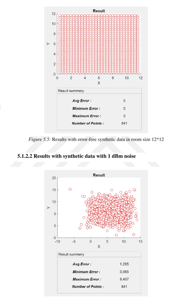
Figure 5.5 Results with error-free synthetic data in room size 12*12 ……….. 27
Figure 5.6 Results with synthetic data with 1dBm in room size 12*12 ……… 27
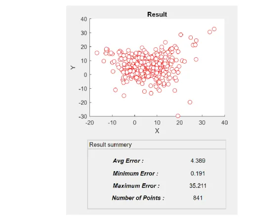
Figure 5.7 Results with synthetic data with 3 dBm in room size 12*12 …………... 28
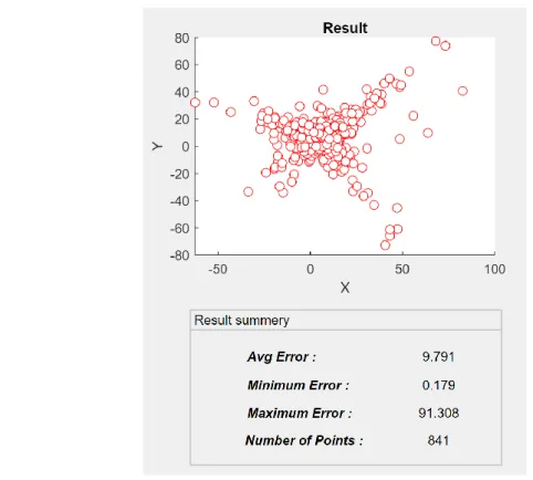
Figure 5.8 Results with synthetic data with 5 dBm in room size 12*12 …………... 29
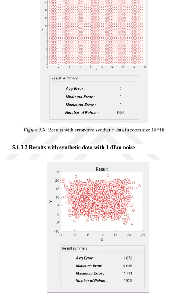
Figure 5.9 Results with synthetic data in room size 18*18 ………... 30
Figure 5.10 Results with synthetic data with 1 dBm in room size 18*18 …………... 30
Figure 5.11 Results with synthetic data with 3 dBm in room size 18*18 …………... 31
Figure 5.12 Results with synthetic data with 5 dBm in room size 18*18……… 32
Figure 5.13 Results with error-free synthetic data in room size 24*24 ……….. 33
Figure 5.14 Results with synthetic data with 1dBm in room size 24*24 ……… 33
Figure 5.15 Results with synthetic data with 3 dBm in room size 24*24 …………... 34
Figure 5.16 Results with synthetic data with 5 dBm in room size 24*24 …………... 35
Figure 5.17 Confidence interval simulation interface ………. 37
Figure 5.18 Impact of noise level ……… 38
Figure 5.19 Impact of noise level with room size ………... 39
Figure 5.20 Impact of noise level with 𝑛 value ………... 39
Figure 5.21 Impact of path loss exponent value ……….. 41
vii
Figure 5.23 Impact of path loss exponent with noise level ………. 42
Figure 5.24 Impact of grid size ………... 43
Figure 5.25 Impact of grid size with room size ……….. 44
Figure 5.26 Impact of grid size with noise level ………. 44
Figure 5.27 Impact of grid size with n value ………... 45
Figure 5.28 Impact of room size ………. 46
Figure 5.29 Impact of room size with noise level ……….. 46
Figure 5.30 Impact of room size with n value ……… 47 Figure 6.1 Results with est. 𝑛 in 6*6 room size with 100cm grid size, 1dBm noise 49 Figure 6.2 Results with est. 𝑛 in 6*6 room size with 60 cm grid size, 1dBm noise 50 Figure 6.3 Results with est. 𝑛 in 6*6 room size with 40 cm grid size, 1dBm noise 50 Figure 6.4 Results with est. 𝑛 in 12*12 room size with 100 cm grid size,1dBm noise 51 Figure 6.5 Results with est. 𝑛 in 12*12 room size with 60 cm grid size, 1dBm noise 52 Figure 6.6 Results with est. 𝑛 in 12*12 room size with 40 cm grid size, 1dBm noise 52 Figure 6.7 Results with est. 𝑛 in 18*18 room size with 100 cm grid size,1dBm noise 53 Figure 6.8 Results with est. 𝑛 in 18*18 room size with 60 cm grid size,1dBm noise 54 Figure 6.9 Results with est. 𝑛 in 18*18 room size with 40 cm grid size,1dBm noise 54 Figure 6.10 Results with est. 𝑛 in 6*6 room size with 100 cm grid size, 3 dBm noise 56 Figure 6.11 Results with est. 𝑛 in 6*6 room size with 60 cm grid size, 3 dBm noise 56 Figure 6.12 Results with est. 𝑛 in 6*6 room size with 40 cm grid size, 3 dBm noise 57 Figure 6.13 Results with est. 𝑛 in 12*12 room size with 100 cm
grid size,
3dBm noise 58 Figure 6.14 Results with est. 𝑛 in 12*12 room size with 60 cm grid size,3dBm noise 58 Figure 6.15 Results with est. 𝑛 in 12*12 room size with 40 cm grid size,3dBm noise 59 Figure 6.16 Results with est. 𝑛 in 18*18 room size with 100 cm grid size,3dBm noise 60 Figure 6.17 Results with est. 𝑛 in 18*18 room size with 60 cm grid size,3dBm noise 60 Figure 6.18 Results with est. 𝑛 in 18*18 room size with 40 cm grid size,3dBm noise 61viii
LIST OF ABBREVIATIONS
GPS The Global Positioning System IPS Indoor Positioning System
IR Infrared
RSS Received Signal Strength AOA Angle of Arrival
TOA Time of Arrival
TDOA Time Difference of Arrival RSSI Received Signal Strength Indicator dBm Decibel-milliwatts AP Access Point RF Radio Frequency LOS Line-of-Sight m Meter CI Confidence Interval
1
1. INTRODUCTION
For thousands of years people have used different ways of localization. They started the basic localization without using any type of special instruments. For instance, the sailors have used celestial objects for sea-based localization. This method involved observing landmarks "sights," or angular measurements taken between a celestial body (the sun, the moon, a planet or a star) and the visible horizon [1].
To provide more accurate localization, many specialized tools have been developed, most notably the astrolabe, sextant, compass as well as maritime charts and maps. The astrolabe was used for many different purposes, including timekeeping during both the day and night, determining the latitude of the user, and calculating the positions of stars, planets and other celestial objects. The sextant is another navigational instrument which relies on mirrors that reflect light along a path to the observer. The sextant mirrors were arranged in such a way that they double the size of the angle that can be measured from one-eighth of a circle to one hundred and twenty (120°) degrees [2].
One of the well-known instruments which were invented more than 2,000 years ago in China, is the compass. A compass is a navigational tool with a magnetic needle (a piece of lodestone) which has its own magnetic field so that, when allowed to rotate freely around its axis, it will align its own magnetic field with that of the Earth and will point towards the magnetic north pole [2]. To use the compass more effectively, maps are used. A map is a graphic representation or scale model of spatial concepts. It is a means for conveying geographic information. The oldest known maps are preserved on Babylonian clay tablets from about 2300 B.C. [3]. Throughout history, maps have evolved. Currently the maps are electronic and they are using satellite for positioning.
In the late 1960s, the U.S. Department of Defense began developing a satellite-based localization system for military purposes, which eventually evolved into the Global Positioning System (GPS). The system was first used in 1990 [4] and became fully operational in 1995.
2
The GPS is a space-based satellite navigation system that provides location and time information for all weather conditions, anywhere on or near the Earth where there is an unobstructed line of sight to three or more GPS satellites [5]. The GPS system consists of up to 24 operational satellites [Figure 1.1] orbiting the Earth on 6 different orbital planes (four to five satellites per plane). The satellites’ orbits are distributed in such a way that from any point on the ground there is line-of-sight contact to at least 4 satellites [6]. Any of these satellites complete its orbit in around 12 hours. Due to the rotation of the Earth, a satellite will be at its initial starting position above the earth’s surface after approximately 24 hours (23 hours 56 minutes to be precise) [6].
Figure1.1: GPS satellites orbit the Earth on 6 orbital planes
The GPS receiver uses the triangulation process to determine physical locations. It communicates with three satellites in sight (using radio signals that travel at the speed of light) and then calculates the distance between those satellites and the device by using the signal travel time. If the distance to the three satellites is known, all possible positions are located on the surface of three spheres whose radius correspond to the distance calculated. The position is the point where all three of the spheres intersect [Figure 1.2].
3
Figure 1.2: The three satellite spheres intersect
Since the satellites have a fixed orbital pattern and are synced with atomic clocks from the U.S. Naval Observatory, this process tends to yield an accurate location reading. But to improve accuracy, GPS devices typically seek data from four or more satellites.
Nowadays with the development of localization technologies and seeing that people spend most of their time in indoor environments, the need for indoor localization has arised. The importance of indoor localization appears more within large buildings. A user can use an Indoor Positioning System (IPS) just like a GPS to be guided to specific destinations. For example, one can use it to find a gate in an airport, specific room or clinic in a hospital, specific chair or facility in a stadium as well as finding a store in a shopping center. Other applications for IPS include real-time tracking, activity recognition, emergency detection and among others [7]. One of the most important uses of indoor localization is in emergencies due to disaster scenarios, such as earthquakes, floods and fires. In these cases, terminals are meant to provide persist exact position within an appropriate lapse of time to the rescuers which will help to save their lives [8].
For localization in outdoor environments, the Global Positioning System (GPS) is used. GPS works extremely well in outdoors but unfortunately, the signal from the GPS satellites are too weak to penetrate most buildings, making GPS useless for indoor localization [5].
4
GPS signals are carried through waves at a frequency that cannot penetrate easily through solid objects and it works better when there is a clear line of sight to the sky. The next generation of positioning technology is being designed to overcome the limitations of GPS. Because of that IPS has become an important research topic.
In previous work, a Received Signal Strength (RSS) based least squares lateration algorithm was introduced [9]. In this thesis, this work is extended by testing the performance of the algorithm based on estimation for many different parameters.
The rest of this thesis is organized as follows: Chapter 2 introduces different techniques for indoor localization and most common IPS algorithms. Chapter 3 describes the Received Signal Strength (RSS) based least squares lateration algorithm. To examine the performance of the algorithm different parameters are used. The experiment description and simulation are described in Chapter 4. Then the simulation results with knowledge of n value introduced in Chapter 5. After that the simulation results with estimated n value shows in Chapter 6. In Chapter 7 the simulation results for the least squares approximation produced. This thesis is completed with conclusions in Chapter 8.
5
2. DIFFERENT TECHNIQUES FOR INDOOR LOCALIZATION
As indoor positioning has become an important research topic, many researches have been done in this field in the last few years. However, most of the techniques, algorithms and constituents of the positioning technologies are not new, as they are also implemented at outdoors. But how they apply to indoors differ from outdoors.
Nowadays, many different Indoor Positioning Systems exist [5]. Some of these systems are:
• Infrared Positioning system: This system uses infrared light pulses (like a TV remote) to locate signals inside a building. Infrared (IR) receivers are installed in every room, and when the IR tag pulses, it is read by the IR receiver device [5]. • Ultrasonic positioning systems: There are three different types of ultrasonic
positioning systems. These are Active bats, Crickets and Dolphin. In these systems the position can be achieved by measuring distances between transmitters and receivers and applying trilateration [5].
• The RSS positioning systems: In the Received Signal Strength (RSS)-based positioning system, the location of the objects can be determined by calculating the distance of the object from the transmitters using triangulation or trilateration techniques.
Positioning systems can be classified by the signal measurement and/or techniques they employ [10]. The dominant techniques for signal measurement are: Angle of Arrival (AOA), Time of Arrival (TOA), Time Difference of Arrival (TDOA) and Received Signal Strength Indicator (RSSI). In this chapter, these techniques will be briefly introduced.
Algorithms used in positioning systems translate recorded signal properties into distances and angles, and then compute the actual position or location of a target object. Thus, a user is able to use the position information in a navigation system during a navigation activity, and the position information can be used to track objects [10]. Triangulation,
6
Trilateration, Proximity and fingerprinting are the algorithms that will be explained later in this chapter.
2.1 Indoor Localization Techniques
2.1.1 Angle of Arrival (AOA)
This technique includes the calculation of the angle at which the signal arrives from the unlocated device to the anchor nodes [11]. The angle and distance are calculated relative to two or multiple reference points through the intersection of direction lines between the reference points [Figure 2.1]. The calculation of the angle and distance are used to estimate and determine the position of a transmitter, and the information is used for tracking or for navigation purposes [10]. The advantage of this technique that it only needs two measuring units for 2D positioning and 3 for 3D. Also, it doesn’t need synchronization between the measuring units. And it works well in situations with LoS (Line of Sight) but the accuracy and precision decrease when there are signal reflections (Multipath). So, it is not good at indoor localization.
Figure 2.1: Positioning based on AOA measurement
2.1.2 Time of Arrival (TOA)
TOA is a distance-based measurement. It calculates the distance between the transmitting node and the receiving node from the transmission time delay and the corresponding speed of signal as follows [7]:
7
where c denotes the traveling speed of the signal, t the amount of time spent by the signal traveling from the transmitting to the receiving node, and d the distance between the transmitting node and the receiving node. Since speed can be regarded as a known constant (usually the speed of light), d can be computed by observing time. TOA provides high accuracy but at a cost of higher hardware complexity [10].
2.1.3 Time Difference of Arrival (TDOA)
TDOA is also a distance-based measurement. TDOA determines the relative position of a transmitter based on the difference in the propagation time of arrival of the transmitter and multiple reference points or sensors [10]. Once the signal is received at two reference points, the difference in arrival time can be used to calculate the difference in distances between the target and the two reference points. This difference can be calculated using the equation:
∆𝑑 = 𝑐 ∗ ∆𝑡 (2.2)
where c is the speed of light and ∆𝑡 is the difference in arrival times at each reference point. TDOA provides high accuracy, and less complexity comparing with TOA.
2.1.4 Received Signal Strength Indicator (RSSI)
RSSI is a measure of the power level of the Received Signal Strength (RSS) present in a radio infrastructure that can be used to estimate the distance between the transmitter node and receiver node [7]. RSSI is typically measured in units of decibel-milliwatts (dBm) which are represented as negative numbers. The closer the values are to 0, the stronger the received signal is. In order to locate an object with the RSSI, the RSSI values between the sensor attached to an object and surrounding access points (APs) with fixed locations are measured. The combination of these multiple RSSI values can be used to calculate the approximate position of the object. Typically, at least 3 access points are required for the localization. The location of the objects is determined by calculating the distance of the object from the transmitters using triangulation or trilateration algorithms [5]. RSSI-based localization is simple to deploy compared to the techniques that use the angle of
8
arrival (AOA) and time difference of arrival (TDOA), there is no need for specialized hardware at the mobile station beside the wireless network interface card [12].
2.2 Indoor Positioning System Algorithms
2.2.1 Triangulation
Triangulation (or angulation) uses the geometric properties of triangles to estimate the position of a target object by computing angular measurements relative to two known reference points [10]. With triangulation, the position of the target node can be determined by the intersection of several pairs of angle direction lines [7], as shown in Figure 2.2 where A and B represent reference nodes, after obtaining the angles 𝜃1, and 𝜃2, the physical position of T (representing the target to be located) could then be calculated based on the predetermined coordinates of the reference nodes.
Figure 2.2: Triangulation algorithm
2.2.2 Trilateration
The trilateration-based positioning algorithm uses three fixed reference nodes to calculate the physical position of a target node [7]. The position of the target object is determined using TOA to measure the time taken by a signal to arrive at a receiver from a transmitter. As seen in Figure 2.3, to find the position of the object T based on the coordinates of three reference nodes: A, B and C and the corresponding distances from each reference node to the target node: R1, R2, and R3, the location of object T can be calculated.
9
Figure 2.3: Trilateration algorithm
This algorithm is currently heavily used in indoor positioning due to its accuracy and low cost. The accuracy depends on the signal received and the environmental conditions. The signal strength received from Wi-Fi access points is commonly used in trilateration for indoor positioning. The advantages of using Wi-Fi networks are that they are becoming much more common, and that the received signal strength is available as part of the networking statistics available on the mobile device. This means that specialist equipment is not required to provide location information [13].
2.2.3 Proximity
The proximity algorithm helps to estimate the location of the target using the proximity relationship between the target and access points (AP). To provide the information, a grid of APs with known positions is used to determine position. When a target (mobile device) is detected in motion, the closest AP is used to calculate its position. But if the mobile device is detected by more than one APs, the AP with the strongest signal is used to calculate its position. The position of the mobile device is determined using RSSI, which is generally used in proximity to estimate the distance between mobile devices in order to acquire the device’s position information [10]. The accuracy of this algorithm is determined by the distribution density and signal range of the access points.
10
2.2.4 Fingerprinting
The basis of this algorithm is constructing a fingerprint database. Fingerprinting approach can be divided into two stages: Sampling (offline) and matching (online) [14]. During the sampling stage, the fingerprint database constructed. This includes a series of steps, such as measuring the site in advance, designing the layout of reference points, and repeating the steps to collect received signal strength (RSS) samples on each reference point. During the matching stage, a location positioning technique uses the currently observed signal strengths and previously collected information to figure out an estimated location. The main challenge to the techniques based on location fingerprints is that the received signal strength could be affected by diffraction, reflection, scattering and absorption during the propagation in indoor environments. The advantages of this algorithm are low cost, a wide range of applications, and good performance.
11
3. THE RECEIVED SIGNAL STRENGTH (RSS) BASED LEAST
SQUARES LATERATION ALGORITHM
Position determination by means of distance measurement using signal strengths is called lateration. This algorithm is used in indoor positioning due to its accuracy and low cost. In this chapter, lateration and least square methods are described.
3.1 Lateration
The lateration method is based on the knowledge of reference point positions and the distances to them. If we have 3 APs and they are located in a room with the following coordinates: AP1 (𝑥1, 𝑦1) , AP2 (𝑥2, 𝑦2) and AP3 (𝑥3, 𝑦3) the distance from each AP to a specific point at coordinate (𝑥, 𝑦) in the room can be found by using the following set of equations: 𝑟1 = √(𝑥1− 𝑥)2 + (𝑦 1− 𝑦)2 (3.1) 𝑟2 = √(𝑥2− 𝑥)2 + (𝑦 2− 𝑦)2 (3.2) 𝑟3 = √(𝑥3− 𝑥)2 + (𝑦3− 𝑦)2 (3.3)
where 𝑟1 is the distance from AP1, 𝑟2 is the distance from AP2 and 𝑟3 is the distance from AP3. Then to find the location of the point (𝑥, 𝑦), the following equations can be derived:
𝑟12 − 𝑟22 = −2𝑥1𝑥 − 2𝑦1𝑦 − 𝑥22 − 𝑦22 + 2𝑥2𝑥 + 2𝑦2𝑦 + 𝑥12 + 𝑦12 (3.4) 𝑟12 − 𝑟32 = −2𝑥1𝑥 − 2𝑦1𝑦 − 𝑥32 − 𝑦32 + 2𝑥3𝑥 + 2𝑦3𝑦 + 𝑥12 + 𝑦12 (3.5)
The Equations (3.4) and (3.5) can be represented as matrix operation as shown in Equation (3.6): [𝑟1 2 − 𝑟 22+ 𝑥22 + 𝑦22 − 𝑥12 − 𝑦12 𝑟12 − 𝑟32+ 𝑥32 + 𝑦32 − 𝑥12 − 𝑦12] = [ 2(𝑥2− 𝑥1) 2(𝑦2− 𝑦1) 2(𝑥3− 𝑥1) 2(𝑦3− 𝑦1)] [ 𝑥 𝑦] (3.6)
12
If we have more than three access points located in a room and we want to use more than 3 APs (says N APs) to increase the accuracy of the estimated location, Equation (3.6) can be extended to N access points as in Equation (3.7):
[ 𝑟12 − 𝑟22+ 𝑥22 + 𝑦22 − 𝑥12 − 𝑦12 𝑟12 − 𝑟32+ 𝑥32 + 𝑦32 − 𝑥12 − 𝑦12 ⋯ 𝑟12 − 𝑟𝑁2+ 𝑥𝑁2 + 𝑦𝑁2 − 𝑥12 − 𝑦12] = [ 2(𝑥2− 𝑥1) 2(𝑦2− 𝑦1) 2(𝑥3− 𝑥1) 2(𝑦3− 𝑦1) ⋯ ⋯ 2(𝑥𝑁− 𝑥1) 2(𝑦𝑁− 𝑦1) ] [𝑥𝑦] (3.7)
From Equation (3.7) we can define 𝐴 and 𝐵 as:
𝐴 = [ 2(𝑥2− 𝑥1) 2(𝑦2− 𝑦1) 2(𝑥3− 𝑥1) 2(𝑦3− 𝑦1) ⋯ ⋯ 2(𝑥𝑁− 𝑥1) 2(𝑦𝑁− 𝑦1) ] (3.8) and 𝐵 = [ 𝑟12 − 𝑟22+ 𝑥22 + 𝑦22 − 𝑥12 − 𝑦12 𝑟12 − 𝑟32+ 𝑥32 + 𝑦32 − 𝑥12 − 𝑦12 ⋯ 𝑟12 − 𝑟 𝑁2+ 𝑥𝑁2 + 𝑦𝑁2 − 𝑥12 − 𝑦12] (3.9)
Then Equation (3.7) can shown as in Equation (3.10) below:
𝐵 = 𝐴 [𝑦] 𝑥 (3.10)
To find the coordinates of the point (𝑥, 𝑦), we solve the equation (3.10) and there is a unique solution for this system as shown in Equation (3.11):
13
3.2 RSSI Measurement:
Received signal strength indicator (RSSI) is defined by the IEEE 802.11 standard [11]. It is a measurement of the radio frequency (RF) energy, and the unit is dBm. The mobile client can get the RSSI from an access point on the WLAN. In indoor environments where it is difficult to obtain line-of-sight (LOS), the RSSI and positioning may be affected by multipath and shadow, hence decreasing accuracy. The RSSI is decreased exponentially as the distance from AP increased, and this can be expressed by the log path loss model. There is a log-normal path loss model for estimation of the distance between receiver and transmitters shown in Equation (3.12) below:
𝑅𝑆𝑆𝐼(𝑑𝐵𝑚) = −10𝑛 𝑙𝑜𝑔(𝑑) + 𝐴 (3.12)
where RSSI is the received signal strength in dBm, d is the true distance from the sender to the receiver in meters, n is the path-loss exponent, and A is received signal strength in dBm at a1-meter distance from the transmitter. Then to calculate the distance of a target from the transmitter, Equation (3.13) can be used:
𝑟 = 10(𝐴−𝑅𝑆𝑆𝐼10 ∗ 𝑛) (3.13)
To calculate A values for the access points, the following procedure can be followed. The received power 1 meter away from each of the four access points is collected over 10 minutes time interval and then the sampled values are averaged [9].
The path loss exponent (n) is one of the most important parameters, which characterizes the power loss of the signal caused by environmental factors. Path loss is intimately related to the environment where the transmitter and receiver are located. Path loss directly affects the link quality of the network and its applications, like distance-based localizations, when the power of the received signal is an important factor [15].
Path loss models are developed using a combination of numerical methods and empirical approximations of measured data collected in channel sounding experiments. It depends on frequency, antenna orientation, penetration losses through walls and floors, the effect
14
of multipath propagation, the interference from other signals, among many other factors [16][17].
In different environments the path loss and standard deviation change based on the environmental conditions. In Table 3.1 the path loss exponent for various environments are presented [15].
Table 3.1: Path loss exponent for different environments Environment Path Loss Exponent
Free Space 2
Urban area cellular radio 2.7 to 3.5 Shadowed urban cellular radio 3 to 5
In building line-of-sight 1.6 to 1.8
Obstructed in buildings 4 to 6
Obstructed in factories 2 to 3
For the calculation of the path loss exponent the following steps are taken [9]:
• In a room of size 6*6 m, a set of 196 reference point, 40 cm apart from each other, determined.
• At each point the RSS values are measured with a sampling interval of 100 milliseconds over a time interval of 1 minute.
• Then the measured values averaged for each access point at each reference point.
• The following matrix (3.14) obtained:
𝑃𝑟 = [ 𝑃𝑟(𝐴𝑃1)1 𝑃𝑟(𝐴𝑃2)1 𝑃𝑟(𝐴𝑃3)1 𝑃𝑟(𝐴𝑃4)1 𝑃𝑟(𝐴𝑃1)2 𝑃𝑟(𝐴𝑃2)2 𝑃𝑟(𝐴𝑃3)2 𝑃𝑟(𝐴𝑃4)2 ⋮ ⋮ ⋮ ⋮ 𝑃𝑟(𝐴𝑃1)196 𝑃𝑟(𝐴𝑃2)196 𝑃𝑟(𝐴𝑃3)196 𝑃𝑟(𝐴𝑃4)196 ] (3.14)
where 𝑃𝑟(𝐴𝑃𝑖)𝑗 is the average RSS value from access point i measured at reference point j.
15
• The distance 𝑟𝑗,𝑖 calculated using Equation (3.15) where 𝑟𝑗,𝑖 represent the distance for reference point j with coordinates (𝑥𝑗, 𝑦𝑗) to 𝐴𝑃𝑖 at coordinates (𝑥𝑖, 𝑦𝑖).
𝑟𝑗,𝑖 = √(𝑥𝑖 − 𝑥𝑗)2 + (𝑦𝑖− 𝑦𝑗)2 (3.15)
Equation (3.15) resulted a distance matrix shown in (3.16):
𝑅 = [ 𝑟1,1 𝑟1,2 𝑟1,3 𝑟1,4 𝑟2,1 𝑟2,2 𝑟2,3 𝑟2,4 ⋮ ⋮ ⋮ ⋮ 𝑟196,1 𝑟196,2 𝑟196,3 𝑟196,4 ] (3.16)
• Then the path loss exponent measured at reference point j for 𝐴𝑃𝑖 is calculated by using Equation (3.17) below:
𝑛 = 𝐴 − 𝑃𝑟(𝐴𝑃𝑖)𝑗 10 log10(𝑟𝑗,𝑖)
(3.17)
Since n value is a constant in the measurement environment, the calculated n values from Equation (3.17) averaged to approximate the path loss exponent using Equation (3.18).
𝑛 ≈ 1 𝑘 × 𝑁∑ ∑ 𝐴 − 𝑃𝑟(𝐴𝑃𝑖)𝑗 10 log10(𝑟𝑗,𝑖) 𝑁 𝑖=1 𝑘 𝑗=1 (3.18)
where k is the number of points in the measurement area. N is the number of access points used.
16
3.3 Least Square Approximation for The RSS Values
Least squares estimation is the standard method to obtain a unique set of values for a set of unknown parameters from a redundant set of observables through a known mathematical model [18]. In particular, the line (the function shown in (3.19), where xi is
the values at which yi is measured and i denotes an individual observation) that minimizes
the sum of the squared distances (deviations) from the line to each observation is used to approximate a linear relationship.
𝑦𝑖 = 𝑏 + 𝑚𝑥𝑖 (3.19)
The graph of the distance with received signal strength in Figure 3.1 shows that the relationship between distance and RSS value is exponentially decreasing which means that when the distance increases the signal strength decreases.
Figure 3.1: The relationship between RSS value and distance
RSSI is usually expressed in decibels relative to a milliwatt (dBm) from zero to -120 dBm. When the RSS value is closer to zero, the signal is stronger. If RSSI level is less than -80 dBm then it is counted as unusable, because of the noise [19]. Table 3.2 shows the signal strength according to the RSSI values.
17
Table 3.2: Signal Strength
RSSI (dBm) Signal strength
> −50 Excellent
-50 to -60 Good
-60 to -70 Fair
< −70 Weak
In indoor localization, the RSS values measured at any reference point is affected by many different factors. Such as the Wi-Fi antenna of the transmitter or receiver and the environment of the measurement area. Because of that data fitting by least squares can be a way to increase the accuracy of the algorithm [9].
In Equation (3.19), xi is represent the distance and yi is represent the RSS values and the
aim is to find m and b to minimize the root mean square error in the approximation of the data {(𝑥𝑖, 𝑦𝑖)} which can be achieved by Equation (3.20):
𝐸 = √1
𝑛∑[𝑏 + 𝑚𝑥𝑖− 𝑦𝑖 ]2 𝑛
𝑖=1
(3.20)
Minimizing E is equivalent to minimizing the sum in Equation (3.20). So, to calculate the minimum value of m and b the following Equations used:
𝑑𝐺(𝑏, 𝑚) 𝑑𝑏 = ∑ 2[𝑏 + 𝑚𝑥𝑖− 𝑦𝑖 ] = 0 𝑛 𝑖=1 (3.21) 𝑑𝐺(𝑏, 𝑚) 𝑑𝑚 = ∑ 2[𝑏 + 𝑚𝑥𝑖 − 𝑦𝑖 ]𝑥𝑖 = 0 𝑛 𝑖=1 (3.22)
18 𝑚 = ∑ 𝑥𝑖𝑦𝑖 𝑛 𝑖=1 − 1 𝑛∑𝑛𝑖=1𝑥𝑖∑𝑛𝑖=1𝑦𝑖 ∑𝑛𝑖=1𝑥𝑖2 − 1𝑛(∑𝑛𝑖=1𝑥𝑖)2 (3.23) 𝑏 = 1 𝑛∑ 𝑦𝑖 𝑛 𝑖=1 − 𝑚 𝑛 ∑ 𝑥𝑖 𝑛 𝑖=1 = 𝑦̅ − 𝑚𝑥̅ (3.24) Let 𝑆𝑥𝑦 = ∑ 𝑥𝑖𝑦𝑖 𝑛 𝑖=1 −1 𝑛∑ 𝑥𝑖 𝑛 𝑖=1 ∑ 𝑦𝑖 𝑛 𝑖=1 (3.25) And 𝑆𝑥𝑥 = ∑ 𝑥𝑖2 𝑛 𝑖=1 − 1 𝑛(∑ 𝑥𝑖 𝑛 𝑖=1 ) 2 (3.26)
Then m and b can be represented as in Equations (3.27) and (3.28) below:
𝑚 =𝑆𝑥𝑦
𝑆𝑥𝑥 (3.27)
𝑏 = 𝑦̅ −𝑆𝑥𝑦
19
4. THE EXPERIMENT DESCRIPTION AND SIMULATION
In order to investigate the performance of RSS-based least squares lateration algorithm for indoor localization under different conditions, I developed a computer simulation using MATLAB for this thesis. This simulation allows the user to enter different parameters and then display the results on the interface. The experiment description and simulation setup will be discussed in this chapter.
4.1 The Experiment Description
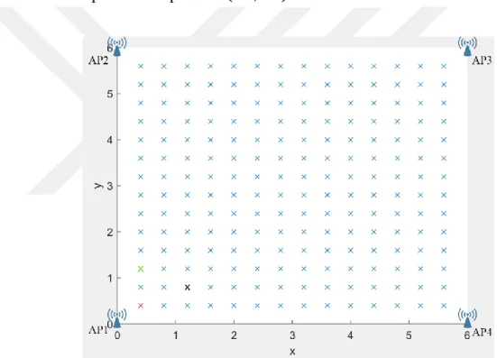
Suppose that we have a measurement area of size (𝑠 × 𝑠) meters. In this area 4 access points are placed at the corners of the measurement area. The coordinates of the APs are: AP1 at coordinate (0,0), AP2 at coordinate (0, 𝑠), AP3 at coordinate (𝑠, 𝑠) and AP4 at coordinate (𝑠, 0). Then the measurement area is divided into grids of size (𝑚 × 𝑚) cm. The corners of this grids marked as reference points as shown in Figure 4.1. Points at edges are ignored since it is unexpected to locate an object at edges as in many cases it is concrete walls. In this measurement area the position of any point can be defined. For example, in Figure 4.1the red point is at position (𝑚, 𝑚), the green point is at position (𝑚, 3𝑚) and the black point in the position (3𝑚, 2 𝑚).
20
These points used in our experiment as reference points to calculate the distance between them and the estimated points which the algorithm will estimate. And then calculate the average error of the position estimation.
As an illustration in Figure 4.2 a measurement area of size (6 × 6) meter used. The grid size is 40 cm. The total number of the marked points is 196 reference point. The access points placed at the following coordinates: AP1 at coordinate (0,0), AP2 at coordinate (0,6), AP3 at coordinate (6,6) and AP4 at coordinate (6,0).
In Figure 4.2 the red point is at position (0.4, 0.4), the green point is at position (0.4, 1.2) and the black point in the position (1.2, 0.8).
Figure 4.2: Measurement area for 6*6 room size and the reference points
4.2 The Simulation Setup
To examine the performance of the algorithm, the simulation interface is designed in a way that allows to test it using different parameters as in Figure 4.3.
The user can choose one of the five room sizes in the list (6*6 m, 12*12 m, 18*18m, 24*24 m, 30*30 m). Sizes bigger than 30*30 m was not added, since it is a very large room and does not exist frequently.
21
Besides the room size the user can choose the grid size from these options (20 cm,30 cm, 40 cm, 50 cm, 60 cm and 100 cm). Additionally, the path loss exponent and the RSS for each access points can be entered. To test the results under different noise levels, the user can enter the noise level and see the calculated results.
The graph, the calculated average error, maximum error, minimum error and number of points generated displayed in the results section of the interface.
Figure 4.3: Simulation interface
When the code is run, first a set of synthetic data is generated according to the room size and grid size parameters. Assuming that each access point is located at a corner of the measurement room. And the number of points generated according to the grid size excluding points at edges.
Then the distance between each point and the four access points calculated. Next the estimated point calculated using Equation (3.11). After that the average error calculated and the results shown on the screen.
Since in real life the signal affected with room furniture and the nature of building materials and most environments contain a noise level, the code was improved by adding
22
a noise when calculating the received signal strength values. To do that a random number from the normal distribution with mean parameter 𝜇 and standard deviation parameter 𝜎 generated using MATLAB function in (4.1).
𝑛𝑜𝑟𝑚𝑟𝑛𝑑(𝜇, 𝜎) (4.1)
After adding different noise levels, the code is run, and the results recorded. The results of the simulation are shown in the following chapters.
23
5. THE SIMULATION RESULTS WITH KNOWLEDGE OF 𝒏
5.1 Results with different room sizes
In each room the simulation is runs 4 times. First the simulation is runs without adding any noise. Then to add noise Equation 5.1 used.
𝑅𝑆𝑆𝐼 𝑚𝑒𝑎𝑠𝑢𝑟𝑒𝑑 = 𝑅𝑆𝑆𝐼𝑖𝑑𝑒𝑎𝑙+ 𝑛𝑜𝑖𝑠𝑒 (5.1) where noise is calculated with mean zero and variance 1,3 or 5 dBm using Equation 4.1. 5.1.1 Results in Room Size 6*6
To run the simulation, the path loss exponent n assumed to be 2.18. and the A values for the four access points assumed to be equaled and the value of A is -50. And 40 cm grid size is used.
5.1.1.1 Results with error-free synthetic data
Figure 5.1 shows that when running the simulation without any noise the average error is equal to 0. The number of points generated is equal to 196.
24
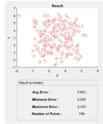
5.1.1.2 Results with synthetic data with 1 dBm noise
Figure 5.2: Results with synthetic data with 1dBm in room size 6*6
Figure 5.2 shows that when adding a 1 dBm noise to the data the average error is 0.603 meter, and the maximum error is 2.4 meter.
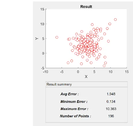
5.1.1.3 Results with synthetic data with 3 dBm noise
As shown in Figure 5.3 when the noise increased the average error also increased. With 3 dBm noise the average error increased to 1.948 m, and the maximum error is 10.363 m.
25
Figure 5.3: Results with synthetic data with 3 dBm in room size 6*6
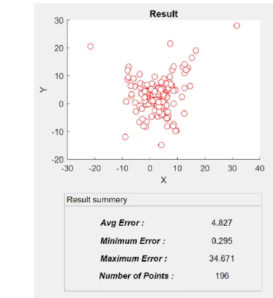
5.1.1.4 Results with synthetic data with 5 dBm noise
When the noise increased to 5 dBm the average error increased a lot. As in Figure 5.4 the average error is 4.8 m, and the maximum error reached 34.67m.
26
Figure 5.4: Results with synthetic data with 5 dBm in room size 6*6
5.1.2 Results in room size 12*12
In this section, the room size changed while the other parameters will be the same. The path loss exponent n assumed to be 2.18. and the A values for the four access points assumed to be equaled and the value of A is -50. And 40 cm grid size is used.
5.1.2.1 Results with error-free synthetic data
When the room size is 12*12 meter and the grid size is 40 cm, 841 points are generated. With error-free synthetic data, the average error calculated is 0. Figure 5.5 shows the distribution of the 841 points.
27
Figure 5.5: Results with error-free synthetic data in room size 12*12
5.1.2.2 Results with synthetic data with 1 dBm noise
28
When the room size is 12 *12 meters with grid size 40 cm and 1 dBm noise, the average error calculated is 1,295 m. The maximum error is 8.407m, and minimum error is 0.065 m as in Figure 5.6.
5.1.2.3 Results with synthetic data with 3 dBm noise
With 3 dBm noise the maximum error reached 35.2 m while the minimum error is 0.191. In this case the average error is 4.39 m. Figure 5.7 shows the results and the estimated point distribution.
Figure 5.7: Results with synthetic data with 3 dBm in room size 12*12
5.1.2.4 Results with synthetic data with 5 dBm noise
Figure 5.8 shows the distribution of the points and the results of synthetic data with 5 dBm noise. The average error is 9.79 m. The minimum error is 0.719 m, and the maximum error is 91.308 m.
29
Figure 5.8: Results with synthetic data with 5 dBm in room size 12*12 5.1.3 Results in room size 18*18
In this section, the room size is changed to a size of 18*18 meter. The other parameters used are the same. The path loss exponent n is assumed to be 2.18. and the A values for the four access points are assumed to be equaled and the value of A is -50. And 40 cm grid size is used.
5.1.3.1 Results with error-free synthetic data
In a room with size 18*18 meter, if the grid size is 40 cm, 1936 points are generated. With error-free synthetic data, the average error calculated is 0. Figure 5.9 shows the distribution of the 841 points.
30
Figure 5.9: Results with error-free synthetic data in room size 18*18
5.1.3.2 Results with synthetic data with 1 dBm noise
31
With 1 dBm noise in a room of size 18*18 m, with 1936 points, the average error is 1.872 m. The minimum error is 0.035 m while the maximum error is 7.731 m. Figure 5.10 shows the results.
5.1.3.3 Results with synthetic data with 3 dBm noise
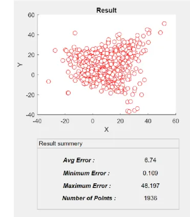
When the noise level is increased to 3 dBm, the maximum error reaches 48.197 m while the minimum error is 0.109. Figure 5.11 shows that the average error is 6.74 m.
Figure 5.11: Results with synthetic data with 3 dBm in room size 18*18
5.1.3.4 Results with synthetic data with 5 dBm noise
Figure 5.12 shows the distribution of the points and the results of synthetic data with 5 dBm noise. The average error is 14.649 m. The minimum error is 0.178 m, and the maximum error is 186.996 m.
32
Figure 5.12: Results with synthetic data with 5 dBm in room size 18*18
5.1.4 Results in Room Size 24*24
Although 24*24 room size considered as big room size and it is only available in large buildings, the algorithm examined with this size. All other parameters used as the previous sections. The path loss exponent n is assumed to be 2.18. and the A values for the four access points are assumed to be equaled and the value of A is -50. And 40 cm grid size is used.
5.1.4.1 Results with error-free synthetic data
With 24*24 room size and 40 cm grid size, the number of points generated is 3481 point. The error-free synthetic data has an average error equal to 0. Figure 5.13 shows the distribution of the 3481 points.
33
Figure 5.13: Results with error-free synthetic data in room size 24*24
5.1.4.2 Results with synthetic data with 1 dBm noise
34
In this case with 1 dBm noise in Figure 5.14, the average error calculated is 2.603 m. The minimum error is 0.051 m, while the maximum error is 12.873 m.
5.1.4.3 Results with synthetic data with 3 dBm noise
With 3 dBm noise the maximum error reaches 82.314 m while the minimum error is 0.072. The average error calculated and found equal to 8.997 m. Figure 5.15 shows the results and the estimated point distribution.
Figure 5.15: Results with synthetic data with 3 dBm in room size 24*24
5.1.4.4 Results with synthetic data with 5 dBm noise
The 5 dBm noise level considered as high noise level. And in a big room with size 24*24 this noise level resulted in a very high average error. Figure 5.16 shows the distribution of the points and the results of synthetic data with 5 dBm noise. The average error is 19.564 m. The minimum error is 0.244 m, and the maximum error is 338.918 m.
35
Figure 5.16: Results with synthetic data with 5 dBm in room size 24*24
5.2 Impact of Different Parameters on The Average Error
In order to examine the impact of different parameters on the average error the confidence interval is used, and the simulation program modified to calculate the confidence interval and to show the results.
In this section, the confidence interval, the simulation modification and the results are discussed.
5.2.1 Confidence interval (CI)
A confidence interval, calculated from a given set of sample data, gives an estimated range of values which is likely to include an unknown population parameter. The CI is expressed as 2 numbers, known as the confidence limits with a range in between. These two numbers are known as upper CI and lower CI. This range, with a certain level of confidence, carries the true but unknown value of the measured variable in the population [20].
36
To calculate the confidence interval first the confidence level should be defined. A confidence level refers to the percentage of all possible samples that can be expected to include the true population parameter [21]. The confidence level is usually set to 95%; hence named "95% confidence interval". In other words, it can be said that this range has a 95% probability of including the true value of the variable [22].
The confidence interval can be calculated using the formula in Equation (5.2) below:
𝑋̅ ± 𝑍 𝑠
√(𝑛) (5.2)
where: 𝑋̅ is the mean, 𝑠 is the standard deviation, 𝑛 is the number of observations and 𝑍 is the value from the 𝑍-table shown in Table 5.1.
The 𝑍-table is short for the “Standard Normal z-table”. The Standard Normal model is used in hypothesis testing, including tests on proportions and on the difference between two means. The area under the whole of a normal distribution curve is 1, or 100 percent. The 𝑍-table helps by telling us what percentage is under the curve at any particular point [21].
Table 5.1: The 𝑍-table
Confidence level 80% 85% 90% 95% 99% 99.5% 99.9%
Z-value 1.282 1.440 1.645 1.960 2.576 2.807 3.291
5.2.2 The simulation modification
To test the impact of different parameters on the average error the simulation interface modified, shown in Figure 5.17, to display a graph of the average error and confidence interval and a table contain the average error, upper CI and lower CI.
Also, the cod has been modified by adding a loop to run the code for 100 times each time the simulation is run. Then the average error results of the 100 runs are averaged and the
37
mean and standard deviation is calculated. The CI then calculated using Equation 5.2. A 95% confidence level is used.
Figure 5.17: Confidence interval simulation interface
5.2.3 The Simulation Results
In this simulation, the impact of following parameters tested: noise level, grid size, room size and the path loss exponent n.
5.2.3.1 Impact of noise level
The algorithm tested with 10 noise level values. The initial parameters used are as following: the room size is 6*6, the grid size is 40 cm, the path loss exponent n is 2 and the A values for the four access points are assumed to be equaled and equal to -50. Figure 5.18 shows the graph of the average error with upper and lower CI. The results are shown in Table 5.2. The results show that when the noise increased, the average error increased.
38
Table 5.2: Impact of noise level
Noise Level (dBm) Average Error (m) Upper CI (m) Lower CI (m)
0.5 0.335 0.337 0.332 1 0.682 0.688 0.676 1.5 1.051 1.063 1.039 2 1.465 1.480 1.449 2.5 1.937 1.962 1.912 3 2.466 2.499 2.433 3.5 3.107 3.151 3.063 4 3.819 3.880 3.758 4.5 4.814 4.892 4.736 5 5.998 6.137 5.859
Figure 5.18: Impact of noise level
5.2.3.1.1 Impact of noise level with room size
The simulation has been run with 5 different room sizes to examine the impact of noise level with room size. The results, in Figure 5.19, shows that when the room size increased with the increasing of the noise level the average error is also increased.
39
Figure 5.19: Impact of noise level with room size
5.2.3.1.2 Impact of noise level with 𝒏 value
The noise level impact tested with 4 different path loss exponent values from Table 3.1. The results show when the noise level increased and the 𝑛 value decreased the average error is increased. Figure 5.20 displays the graph of these results.
40
5.2.3.2 Impact of path loss exponent
The simulation runs to test the impact of path loss exponent. Based on Table 3.1, 6 different n values used in the simulation. The initial parameters used as follows: room size 6*6, grid size 40 cm, noise level 1 dBm and the A values for the four access points are assumed to be equaled and equal to -50.
The results show that when the path loss exponent increased the average error decreased. Which means there is an inverse relationship between path loss exponent and the average error calculated.
Table 5.3 and Figure 5.21 show the results.
Table 5.3: Impact of path loss exponent value
𝒏 value Average Error (m) Upper CI (m) Lower CI (m)
1.6 0.865 0.871 0.859 1.8 0.76 0.766 0.754 2 0.674 0.679 0.669 2.7 0.494 0.498 0.49 3 0.448 0.452 0.444 3.5 0.384 0.387 0.381 4 0.334 0.337 0.331 5 0.267 0.269 0.265 6 0.221 0.223 0.219
41
Figure 5.21: Impact of path loss exponent value
5.2.3.2.1 Impact of path loss exponent with room size
The simulation has been run with 5 different room sizes to examine the impact of path loss exponent with room size. The room sizes used as follows: 6*6, 12*12, 18*18, 24*24 and 30*30. The results, in Figure 5.22, shows that when the room size increased with the increasing of the path loss exponent the average error is decreased.
42
5.2.3.2.2 Impact of path loss exponent with the noise level
To examine the impact of path loss exponent with the noise level, 5 noise level used as in Figure 5.23. the results show that as the 𝑛 value increased and the increasing of noise level, the average error decreased.
Figure 5.23: Impact of path loss exponent with the noise level 5.2.3.3 Impact of grid size
To test the impact of grid size the algorithm tested with 5 different grid sizes. Changing the grid size affect the number of points generated. For example, in a room of size 6*6 using 40 cm grid generates 196 points while in the same room if 20 cm grid size used, 841 points are generated. The initial parameters used are as following: the room size is 6*6, the noise level is 1 dBm, the path loss exponent n is 2 and the A values for the four access points are assumed to be equaled and equal to -50.
Figure 5.24 shows the graph of the average error with upper and lower CI. Although the graph seems like a decreasing graph, the results numbers in Table 5.4 shows that the average error decreased in a very small range.
43
Table 5.4: Impact of grid size
Grid Size (cm) Average Error (m) Upper CI (m) Lower CI (m)
20 0.695 0.698 0.692
30 0.691 0.695 0.687
40 0.678 0.684 0.672
50 0.674 0.681 0.667
60 0.668 0.676 0.66
Figure 5.24: Impact of grid size
5.2.3.3.1 Impact of grid size with room size
The simulation has been run with 5 different room sizes to examine the impact of grid size with room size. The room sizes used as follows: 6*6, 12*12, 18*18, 24*24 and 30*30. The results, in Figure 5.25, shows that when the grid size increased with the increasing of the room size the average error is almost a constant.
44
Figure 5.25: Impact of grid size with room size
5.2.3.3.2 Impact of grid size with noise level
To examine the impact of grid size with noise level, 5 noise levels are used as in Figure 5.26. The results show that as the grid size increased with the increasing of noise level, the average error is almost a constant.
45
5.2.3.3.3 Impact of grid size with 𝒏 value
In order to examine the impact of grid size with 𝑛 value, 5 𝑛 values from Table 3.1 is used. Figure 5.27 shows that when the grid size increased the average error is almost a constant. While when decreasing the 𝑛 value the average error increased.
Figure 5.27: Impact of grid size with 𝑛 value
5.2.3.4 Impact of room size
The simulation has been run to explore the algorithm performance in different room sizes. The sizes used as follows: 6*6, 12*12, 18*18, 24*24 and 30*30. Although 30*30 meter is very big room size, it was added to inspect the impact of room size. The initial parameters used are as following: The grid size is 40 cm, the noise level is 1 dBm, the path loss exponent n is 2 and the A values for the four access points are assumed to be equaled and equal to -50. As seen in Table 5.5 and Figure 5.28, the results of this simulation show that when the room size increased the average error also increased.
46
Table 5.5: Impact of room size
Room size (m) Average Error (m) Upper CI (m) Lower CI (m)
6*6 0.676 0.682 0.67
12*12 1.391 1.397 1.385
18*18 2.097 2.103 2.091
24*24 2.807 2.813 2.801
30*30 3.517 3.523 3.511
Figure 5.28: Impact of room size 5.2.3.4.1 Impact of room size with the noise level
To examine the impact of room size with noise level, 5 noise levels are used as in Figure 5.29. The results show that as the room size increased with the increasing of noise level, the average error is increased.
47
5.2.3.4.2 Impact of room size with 𝒏 value
In order to examine the impact of room size with 𝑛 value, 5 different 𝑛 values from Table 5.3 are used. Figure 5.30 shows that when the room size increased and the 𝑛 value decreased, the average error increased.