Diffusion Equation Including Local Fractional Derivative And Non-Homogenous Dirichlet Boundary Conditions

(1)

RESEARCH ARTICLE

101

DIFFUSION EQUATION INCLUDING LOCAL FRACTIONAL DERIVATIVE AND NON-HOMOGENOUS DIRICHLET BOUNDARY CONDITIONS

Süleyman ÇETİNKAYA1_{, Ali DEMİR}2

1

Kocaeli University, Faculty of Arts and Sciences, Department of Mathematics, 41380, Kocaeli,

suleyman.cetinkaya@kocaeli.edu.tr, ORCID: 0000-0002-8214-5099 2

Kocaeli University, Faculty of Arts and Sciences, Department of Mathematics, 41380, Kocaeli, ademir@kocaeli.edu.tr, ORCID: 0000-0003-3425-1812

Received Date: 30.10.2020 Accepted Date: 07.12.2020

ABSTRACT

In this research, we discuss the construction of analytic solution of non-homogenous initial boundary value problem including PDEs of fractional order. Since non-homogenous initial boundary value problem involves local fractional derivative, it has classical initial and boundary conditions. By means of separation of variables method and the inner product defined on 𝐿2_{[0, 𝑙], the solution is constructed}

in the form of a Fourier series with respect to the eigenfunctions of a corresponding Sturm-Liouville eigenvalue problem including local fractional derivative used in this study. Illustrative example presents the applicability and influence of separation of variables method on fractional mathematical problems.

Keywords: Local fractional derivative, Time-fractional diffusion equation, Initial-boundary-value

problems, Spectral method, Non-homogenous Dirichlet boundary conditions

1. INTRODUCTION

Since mathematical models including fractional derivatives play a vital role fractio nal derivatives draw a growing attention of many researchers in various branches of sciences. Therefore there are many different fractional derivatives such as Caputo, Riemann-Liouville, Atangana-Baleanu. However these fractional derivatives don’t satisfy most important properties of ordinary derivative which leads to many diffuculties to analyze or obtain the solution of fractional mathematical models. As a result many scientists focus on defining new fractional derivatives to cover the setbacks of the defined ones. Moreover the success of mathematical modelling of systems or processes depends on the fractional derivative, it involves, since the correct choice of the fractional derivative allows us to model the real data of systems or processes accurately.

In order to the define new fractional derivatives, various methods exists and these ones are classfied based on their features and formation such as nonlocal fractional derivatives and local fractional derivatives. From a physical aspect, the intrinsic nature of the physical system can be reflected to the

(2)

Çetinkaya S. and Demir A., Journal of Scientific Reports-A, Number 45, 101-110, December 2020.

102

mathematical model of the system by using fractional derivatives. Therefore the solution of the fractional mathematical model is in excellent agreement with the predictions and experimental measurement of it. The systems whose behaviour is non-local can be modelled better by fractional mathematical models and the degree of its non-locality can be arranged by the order of fractional derivative. In order to analyze the diffusion in a non-homogenous medium that has memory effects it is better to analyze the solution of the fractional mathematical model for this diffusion. As a result in order to model a process, the correct choices of fractional derivative and its order must be determined. Rheology is known as the scientific study of material diffusion. In rheology, mathematical models of diffusion process are employed to analyze the behaviour of materials which allow us to classify and compare them. In this study, we focus on fractional diffusion problem including time fractional derivative. The novelty of this research is that the materials can be classified as liquid, gas and temperature based on the order of time fractional derivative. For instance, fractional diffusion model of materials which behaves slower, the order of time fractional derivative is between zero and one and the order of time fractional derivative for materials which behaves faster is greater than one. Moreover based on the complexity of the material, suitable fractional derivative need to be chosen to facilitate the correct analysis of the material. In this study, we classify non-complex materials therefore local fractional derivative is used. Mathematical model of diffusion problems including local fractional derivatives gives better results than ones including integer order derivatives [1]. There are many published work on the diffusion of various matters in science especially in fluid mechanics and gas dynamics [2-7].

2. MAIN RESULTS

The proportional derivative is a newly defined fractional derivative which is generally defined as 𝐷_𝛼

𝑃 _{𝑓(𝑡) = K}

1(α,t) f(t) + K0(α,t)f′(t), (1)

where the functions 𝐾0 and 𝐾1 satisfy certain properties in terms of limit [8] and 𝑓 is a differentiable

function. Notice that this derivative can be regarded as an extension of conformable derivative and is used in control theory.

In this study we focus on obtaining the solution of following fractional diffusion equation including various proportional derivative operator by making use of the separation of variables method:

𝐷_𝑡𝛼

𝑃 _{𝑢(𝑥, 𝑡) = γ}2_𝑢

𝑥𝑥(𝑥, 𝑡), (2)

𝑢(0, 𝑡) = 𝑢₀,𝑢(𝑙, 𝑡) = 𝑢₁, (3)

𝑢(𝑥, 0) = 𝑓(𝑥) (4)

where 0 < α < 1, γ ∈ ℝ,0 ≤ 𝑥 ≤ 𝑙, 0 ≤ 𝑡 ≤ 𝑇, 𝑢₀ and 𝑢₁ are constants. Here we use the following forms of the proportional derivatives:

𝐷_𝛼

𝑃 _{𝑓(𝑡) = 𝐾}

1(𝛼) 𝑓(𝑡) + 𝐾0(𝛼)𝑓′(𝑡). (5)

Especially we consider the following ones: 𝐷

1 𝑃

(3)

Çetinkaya S. and Demir A., Journal of Scientific Reports-A, Number 45, 101-110, December 2020. 103 and 𝐷 2 𝑃 α𝑓(𝑡) = (1 − α2) 𝑓(𝑡) + α2𝑓′(𝑡). (7)

Let us consider the following problem including the proportional derivative in (6) 𝐷_𝑡𝛼

𝑃 _{𝑢(𝑥, 𝑡) = γ}2_𝑢

𝑥𝑥(𝑥, 𝑡), (8)

𝑢(0, 𝑡) = 𝑢₀,𝑢(𝑙, 𝑡) = 𝑢₁, (9)

𝑢(𝑥, 0) = 𝑓(𝑥), (10)

where 0 < 𝛼 < 1, 𝛾 ∈ ℝ, 0 ≤ 𝑥 ≤ 𝑙, 0 ≤ 𝑡 ≤ 𝑇, 𝑢₀ and 𝑢₁ are constants.

Before investigating the solution of the problem (8)-(10), let us define the function 𝑣(𝑥, 𝑡) which homogenizes boundary conditions (9) as follows:

𝑣(𝑥, 𝑡) = 𝑢(𝑥, 𝑡) +𝑥

𝑙(𝑢0− 𝑢1) − 𝑢0. (11)

Via (11), the problem (8)-(10) turns into the following problem (12)-(14). 𝐷_𝑡𝛼

𝑃 _{𝑣(𝑥, 𝑡) = γ}2_𝑣

𝑥𝑥(𝑥,𝑡), (12)

𝑣(0, 𝑡) = 0, 𝑣(𝑙, 𝑡) = 0 (13)

𝑣(𝑥, 0) = 𝑓(𝑥) +𝑥_𝑙(𝑢₀− 𝑢₁) − 𝑢₀, (14)

where 0 < 𝛼 < 1, 𝛾 ∈ ℝ, 0 ≤ 𝑥 ≤ 𝑙, 0 ≤ 𝑡 ≤ 𝑇, 𝑢₀ and 𝑢₁ are constants.

By means of separation of variables method, The generalized solution of above problem is constructed in analytical form. Thus a solution of problem (12)-(14) have the following form:

𝑣(𝑥, 𝑡; α) = 𝑋(𝑥)𝑇(𝑡;α) (15)

where 0 ≤ 𝑥 ≤ 𝑙, 0 ≤ 𝑡 ≤ 𝑇.

Plugging (15)into (12) and arranging it, we have

𝐷 𝑃 𝑡α(𝑇(𝑡;α)) 𝑇(𝑡;α) = γ 2 𝑋′′(𝑥) 𝑋(𝑥) = −λ 2_. ₍₁₆₎

Equation (16) produce a fractional differential equation with respect to time and an ordinary differential equation with respect to space. The first ordinary differential equation is obtained by taking the equation on the right hand side of Eq. (16). Hence with boundary conditions (13), we have the following problem:

𝑋′′(𝑥) + 𝜆2_{𝑋(𝑥) = 0,} ₍₁₇₎

𝑋(0) = 𝑋(𝑙) = 0. (18)

The solution of eigenvalue problem (17)-(18) is accomplished by making use of the exponential function of the following form:

(4)

104

𝑋(𝑥) = 𝑒𝑟𝑥_. ₍₁₉₎

Hence the characteristic equation is computed in the following form:

𝑟2_{+ 𝜆}2_{= 0.} ₍₂₀₎

Case 1: If 𝜆 = 0, then the characteristic equation have coincident solutions 𝑟_1,2= 0, leading to the general solution of the eigenvalue problem (17)-(18) have the following form:

𝑋(𝑥) = 𝑘₁𝑥 + 𝑘₂.

The first boundary condition yields

𝑋(0) = 𝑘₂= 0 ⇒ 𝑘₂= 0. (21)

which leads to the following solution

𝑋(𝑥) = 𝑘₁𝑥. (22)

Similarly second boundary condition leads to

𝑋(𝑙) = 𝑘₁𝑙 = 0 ⇒ 𝑘₁= 0. (23)

which implies that

𝑋(𝑥) = 0. (24)

As a result, the characteristic equation (20) can not have the solution 𝜆 = 0.

Case 2. If 𝜆 > 0, the Eq. (20) have two distinct real roots 𝑟₁, 𝑟₂ yielding the general solution of the problem (17)-(18) in the following form:

𝑋(𝑥) = 𝑐₁𝑒𝑟1𝑥+ 𝑐₂𝑒𝑟2𝑥_. ₍₂₅₎

By making use of the first boundary condition, we have

𝑋(0) = 𝑐₁+ 𝑐₂= 0. 𝑐₁= −𝑐₂. (26)

From second boundary condition

𝑋(𝑙) = (−𝑐2)𝑒𝑟1𝑙+ 𝑐2𝑒𝑟2𝑙= 𝑐2(−𝑒𝑟1𝑙+ 𝑒𝑟2𝑙) = 0

Which indicates that 𝑐₂= 0. Hence 𝑐₁= 0 which implies that 𝑋(𝑥) = 0 which implies that there is not any solution for 𝜆 > 0.

(5)

105

𝑟_1,2= ∓𝑖𝜆 (27)

which leads to the general solution of the eigenvalue problem (17)-(18) have the following form:

𝑋(𝑥) = 𝑐1cos(𝜆𝑥) + 𝑐2sin(𝜆𝑥). (28)

By making use of the first boundary condition we have

𝑋(0) = 𝑐₁= 0 ⇒ 𝑐₁= 0. (29)

Hence the solution becomes

𝑋(𝑥) = 𝑐₂sin(𝜆𝑥). (30)

Similarly last boundary condition leads to

𝑋(𝑙) = 𝑐₂sin(𝜆𝑙) = 0 (31)

which implies that

sin(𝜆𝑙) = 0. (32)

Let 𝑤_𝑛= λ_nl. The solutions of (32) can be denoted by means of 𝑤_𝑛= 𝑛𝜋, 𝑛 = 0,1,2,3, … which are eigenvalues of the problem (17)-(18), as follows:

𝜆_𝑛=𝑤𝑛2

𝑙2, 0 < 𝑤1< 𝑤2< 𝑤3< ⋯ , 𝑛 = 0,1,2,3, … (33)

As a result the solution is obtained as follows:

𝑋_𝑛(𝑥) = 𝑐_𝑛sin (𝑤_𝑛(𝑥_𝑙)) = sin (𝑤_𝑛(𝑥_𝑙)), 𝑛 = 0,1,2,3, … (34) The second equation in (16) for eigenvalue 𝜆_𝑛 yields the ordinary differential equation below:

𝐷 𝑃 𝑡α(𝑇(𝑡;𝛼)) 𝑇(𝑡;𝛼) = −𝛾 2_𝜆2_, ₍₃₅₎ 𝐾1(α) 𝑇𝑛(𝑡;𝛼)+𝐾0(α)𝑇𝑛′(𝑡;𝛼) 𝑇𝑛(𝑡;𝛼) = −𝛾 2_𝜆 𝑛 2_, 𝐾0(α)𝑇𝑛′(𝑡; 𝛼) + (𝛾2𝜆2𝑛+ 𝐾1(α))𝑇𝑛(𝑡; 𝛼) = 0

which yields the following solution 𝑇_𝑛(𝑡;𝛼) = 𝑒𝑥𝑝 (−𝛾2𝜆𝑛2+𝐾1(α)

𝐾₀(α) 𝑡), 𝑛 = 0,1,2,3, … (36)

(6)

Çetinkaya S. and Demir A., Journal of Scientific Reports-A, Number 45, 101-110, December 2020. 106 𝑣_𝑛(𝑥, 𝑡; 𝛼) = 𝑋_𝑛(𝑥)𝑇_𝑛(𝑡;𝛼) = 𝑒𝑥𝑝 (−𝛾2𝜆𝑛2+𝐾1(α) 𝐾0(α) 𝑡) sin (𝑤𝑛( 𝑥 𝑙)), 𝑛 = 1,2,3, … (37)

which leads to the following general solution 𝑣(𝑥, 𝑡; 𝛼) = ∑ 𝑑_𝑛sin (𝑤_𝑛(𝑥 𝑙)) ∞ 𝑛=1 𝑒𝑥𝑝 (−𝛾 2_𝜆 𝑛 2_+𝐾 1(α) 𝐾0(α) 𝑡). (38) Note that it satisfies boundary condition and fractional differential equation.

The coefficients of general solution are established by taking the following i nitial condition into account: 𝑣(𝑥, 0) = 𝑓(𝑥)+𝑥 𝑙(𝑢0− 𝑢1) − 𝑢0= ∑ 𝑑𝑛sin (𝑤𝑛( 𝑥 𝑙)) ∞ 𝑛=1 . (39)

The coefficients 𝑑_𝑛 for 𝑛 = 0,1,2,3, … determined by the help of inner product defined on 𝐿2_{[0, 𝑙]:}

𝑑_𝑛=2 𝑙[∫ sin( 𝑛𝜋𝑥 𝑙 )𝑓(𝑥)𝑑𝑥 𝑙 0 + (𝑢0− 𝑢1)∫ sin ( 𝑛𝜋𝑥 𝑙 ) 𝑥 𝑙𝑑𝑥 𝑙 0 − 𝑢0∫ sin ( 𝑛𝜋𝑥 𝑙 ) 𝑑𝑥 𝑙 0 ]. (40)

Substituting (40) in (38) leads to the solution of the problem (12)-(14). By making use of (11) and this solution we obtain the general solution of the problem (8)-(10).

𝑢(𝑥, 𝑡) = 𝑢0+𝑥_𝑙(𝑢1− 𝑢0) + ∑∞𝑛=1𝑑𝑛sin(𝑤𝑛(𝑥_𝑙))𝑒𝑥𝑝 (−𝛾 2_𝜆 𝑛 2_+𝐾 1(α) 𝐾0(α) 𝑡). (41) If 𝛾2 is replaced by the fractional diffusion coefficient 𝑐2𝜏_𝛼1−𝛼 where 𝑐2 is ordinary diffusion coefficient and τ_𝛼 is a time constant the solution takes the following form:

𝑢(𝑥, 𝑡; 𝛼) = 𝑢₀+𝑥 𝑙(𝑢1− 𝑢0) + ∑ 𝑑𝑛sin (𝑤𝑛( 𝑥 𝑙)) ∞ 𝑛=1 𝑒𝑥𝑝 (−𝑐 2_𝜏 𝛼 1−𝛼_𝜆 𝑛 2_+𝐾 1(α) 𝐾0(α) 𝑡). (42) 3. ILLUSTRATIVE EXAMPLE

In this section, we first consider the following non-homogenous initial boundary value problem: 𝑢_𝑡(𝑥, 𝑡) = 𝑢_𝑥𝑥(𝑥, 𝑡),

𝑢(0, 𝑡) = 1 , 𝑢(2, 𝑡) = 1,

𝑢(𝑥, 0) = − sin(𝜋𝑥)+ 1 (43)

which has the solution in the following form:

𝑢(𝑥, 𝑡) = −sin(𝜋𝑥)𝑒−𝜋2𝑡_{+ 1} ₍₄₄₎

where 0 ≤ 𝑥 ≤ 2, 0 ≤ 𝑡 ≤ 𝑇.

Example 1. Now let the following problem called fractional heat-like problem be taken into consideration:

(7)

Çetinkaya S. and Demir A., Journal of Scientific Reports-A, Number 45, 101-110, December 2020. 107 𝐷 1 𝑃 𝑡 α_{𝑢(𝑥, 𝑡) = 𝑢} 𝑥𝑥(𝑥, 𝑡), 𝑃𝑡α(𝑥,𝑡)=𝑢𝑥𝑥(𝑥,𝑡), (45) 𝑢(0, 𝑡) = 1, 𝑢(2, 𝑡) = 1, (46) 𝑢(𝑥, 0) = − sin(𝜋𝑥) + 1 (47) where 0 < 𝛼 < 1, 0 ≤ 𝑥 ≤ 2, 0 ≤ 𝑡 ≤ 𝑇.

To make the boundary condition (46) homogenous, we apply the transformation

𝑣(𝑥, 𝑡) = 𝑢(𝑥, 𝑡) − 1 (48)

to the above problem which leads to the following fractional heat-like problem 𝐷 1 𝑃 𝑡 α_{𝑣(𝑥, 𝑡) = 𝑣} 𝑥𝑥(𝑥, 𝑡), 𝑃𝑡α(𝑥,𝑡)=𝑣𝑥𝑥(𝑥,𝑡), (49) 𝑣(0, 𝑡) = 0 , 𝑣(2, 𝑡) = 0, (50) 𝑣(𝑥, 0) = − sin(𝜋𝑥) (51)

where 0 < 𝛼 < 1, 0 ≤ 𝑥 ≤ 2, 0 ≤ 𝑡 ≤ 𝑇. It is clear from Eq. (38) that the solution of above problem can be obtained in the following form:

𝑣(𝑥, 𝑡; 𝛼) = ∑∞ 𝑑_𝑛sin (𝑛π𝑥₂ )

𝑛=1 𝑒𝑥𝑝 (−𝑛

2_π2_+4−4𝛼

4α 𝑡). (52)

Plugging 𝑡 = 0 in to the general solution (52) and making equal to the initial condition (51) we have − sin(π𝑥) = ∑ 𝑑_𝑛sin (𝑛π𝑥

2 ) ∞

𝑛=1 . (53)

The coefficients 𝑑_𝑛 for 𝑛 = 0,1,2,3, … are determined by the help of the inner product as follows: 𝑑_𝑛= ∫ − sin (₀2 𝑛𝜋𝑥₂ ) sin(𝜋𝑥) 𝑑𝑥.

𝑑_𝑛= 0 for 𝑛 ≠ 2. For 𝑛 = 2, 𝑑₂ is obtained as follows: ⟹ 𝑑₂= − ∫ sin2 2_{(𝜋𝑥)𝑑𝑥} 0 = − 1 2(𝑥 + sin(2𝜋𝑥) 4𝜋 )|𝑥=0 𝑥=2 = −1. (54)

Substituting (54) in (52) leads to the solution of the problem (49)-(51). 𝑣(𝑥, 𝑡; 𝛼) = − sin(𝜋𝑥)𝑒𝑥𝑝 (−π2+1−𝛼

α 𝑡). (55)

By making use of (48) and the solution (55), we obtain the general solution of the problem (45)-(47) as follows:

u(𝑥, 𝑡; α) = − sin(π𝑥) exp (−π2+1−α

α 𝑡) + 1. (56)

It is important to note that plugging 𝛼 = 1 in to the solution (56) gives the solution (44) which confirm the accuracy of the method we apply.

(8)

108

Example 2. Now let the following problem called fractional heat-like problem be taken into consideration: 𝐷 2 𝑃 𝑡 α_{𝑢(𝑥, 𝑡) = 𝑢} 𝑥𝑥(𝑥, 𝑡), 𝑃𝑡α(𝑥,𝑡)=𝑢𝑥𝑥(𝑥,𝑡), (57) 𝑢(0, 𝑡) = 1, 𝑢(2, 𝑡) = 1, (58) 𝑢(𝑥, 0) = − sin(𝜋𝑥) + 1 (59)

where 0 < 𝛼 < 1, 0 ≤ 𝑥 ≤ 2, 0 ≤ 𝑡 ≤ 𝑇. To make the boundary condition (58) homogenous, we apply the transformation

𝑣(𝑥, 𝑡) = 𝑢(𝑥, 𝑡) − 1 (60)

to the above problem which leads to the following fractional heat-like problem 𝐷 2 𝑃 𝑡 α_{𝑣(𝑥, 𝑡) = 𝑣} 𝑥𝑥(𝑥, 𝑡), 2𝑃𝑡α(𝑥,𝑡)=𝑣𝑥𝑥(𝑥,𝑡), (61) 𝑣(0, 𝑡) = 0 , 𝑣(2, 𝑡) = 0, (62) 𝑣(𝑥, 0) = − sin(𝜋𝑥) (63)

where 0 < 𝛼 < 1, 0 ≤ 𝑥 ≤ 2, 0 ≤ 𝑡 ≤ 𝑇. It is clear from Eq. (38) that the solution of above problem can be obtained in the following form:

𝑣(𝑥, 𝑡; 𝛼) = ∑ 𝑑_𝑛sin (𝑛π𝑥 2 ) ∞ 𝑛=1 𝑒𝑥𝑝 (−𝑛 2_π2_+4−4α2 4α2 𝑡). (64)

As in Example 1, after similar computations the solution can be constructed as follows: u(𝑥, 𝑡; α) = − sin(π𝑥) exp (−π2+1−α2

α2 𝑡) + 1. (65)

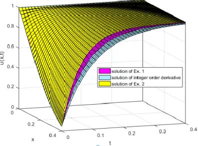
It is important to note that plugging 𝛼 = 1 in to the solution (65) gives the solution (44) which confirm the accuracy of the method we apply. The graphics of solutions, obtained by MATLAB 2016b, for Ex.1, Ex. 2 and Problem (43) in 2D and 3D are given in Fig.1 and Fig.2 respectively.

(9)

109

Figure 1. The graphics of solutions for Ex. 1 and Ex. 2. in 2D at x=0.1 for α = 0.8.

Figure 2. The graphics of solutions for Ex. 1 and Ex. 2 in 3D for α = 0.8. 4. CONCLUSION

In this study, the analytic solution of time fractional diffusion problem including local fractional derivatives in one dimension is constructed analytically in Fourier series form. Taking the separation of variables into account, the solution is formed in the form of a Fourier series with respect to the

(10)

110

eigenfunctions of a corresponding Sturm-Liouville eigenvalue problem including fractional derivative in a proportional sense.

Based on the analytic solution, we reach the conclusion that diffusion processe s decays exponential with time until initial condition is reached. As α tends to 0, the rate of decaying increases. This implies that in the mathematical model for diffusion of the matter which has small diffusion rate the value of α must be close to 0. This model can account for various diffusion processes of various methods.

REFERENCES

[1] Hao, Y.J., Srivastava, H. M., Jafari, H., Yang, X.J., (2013), Helmholtz and di usion equations associated with local fractional derivative operators involving the Cantorian and Cantor-type cylindrical coordinates, Advances in Mathematical Physics, 2013, Article ID 754248, 1-5.

[2] Bisquert, J., (2005), Interpretation of a fractional diffusion equation with non-conserved probability density in terms of experimental systems with trapping or recombination, Physical Review E, 72(1), 011109.

[3] Sene, N., (2019), Solutions of Fractional Diffusion Equations and Cattaneo -Hristov Diffusion Model, International Journal of Analysis and Applications, 17(2), 191-207.

[4] Aguilar, J.F.G. and Hernández, M.M., (2014), Space-Time Fractional Diffusion-Advection Equation with Caputo Derivative, Abstract and Applied Analysis, 2014, Article ID 283019 . [5] Naber, M., (2004), Distributed order fractional sub-diffusion, Fractals, 12(1), 23-32.

[6] Nadal, E., Abisset-Chavanne, E., Cueto, E. and Chinesta, F., (2018), On the physical interpretation of fractional diffusion, Comptes Rendus Mecanique, 346, 581 -589.

[7] Zhang, W. and Yi, M., (2016), Sturm-Liouville problem and numerical method of fractional diffusion equation on fractals, Advances in Difference Equations, 2016:217.

[8] Baleanu, D., Fernandez, A. and Akgül, A., (2020), On a Fractional Operator Combining Proportional and Classical Differintegrals, Mathematics, 8(360).