Selçuk J. Appl. Math. Selçuk Journal of Special Issue. pp. 53-60, 2011 Applied Mathematics
LS-SVM Method for Fuzzy Nonlinear Regression Ümran M. Tek¸sen1, A¸sır Genç
Selcuk University, Faculty of Science, Department of Statistics, 42003, Campus, Konya, Turkiye.
e-mail: uteksen@ gm ail.com,agenc@ selcuk.edu.tr
Abstract. In this study LS-SVM method is applied for fuzzy nonlinear re-gression whose input and output are fuzzy numbers. The method solves any problem of classification or regression via transforming to a quadratic problem without running into local solutions. This method is favourable owing to inde-pendent from a model. In this study, two practises are applied to linear and nonlinear data.
Key words: Fuzzy Nonlineer Regression, Least Squares Support Vector Ma-chine
2000 Mathematics Subject Classification: 26D15. 1. Introduction
Fuzzy regression model is used for obtaining functional relationship between dependent and independent variables in a fuzzy environment. Fuzzy linear re-gression presents a fuzzy linear model describing functional relationship between input-output pairs. However, this assumption causes lots of modelling mistakes in nonlinear case. Fuzzy nonlinear regression methods are offered eliminating these disadvantages. In practise, relationship between input-output pairs usu-ally is not known. Therefore, fuzzy regression without a model is needed (Hong and Hwang, 2006).
Initially fuzzy regression is improved for linear relationship. Tanaka et al. (1982) implemented fuzzy linear regression to crisp data. After, they obtained fuzzy regression via using fuzzy input data which consist of triangular fuzzy numbers. Dubois and Prade (1980) also explained this method. Ishibuchi and Tanaka (1992) offered a simple but strong method using artificial neural networks for fuzzy regression. They reduced fuzzy regression analyse to interval regression analyse and described with training two independent neural networks whose lower and upper bounds of output interval. Xu et al. (2000) aimed estimating interval for nonlinear fuzzy regression.
In this study, fuzzy nonlinear regression is studied for fuzzy input- fuzzy output data. In fuzzy nonlinear regression analyse Least Squares Support Vector Ma-chine (LS-SVM) method which is proposed by Hong and Hwang (2006) is used because of being intended a method without a model.
In recent years, Support Vector Machines (SVM) are commonly used algorithms. SVMs basically depend on obtaining maximum margin for decision surface of two classes which are linear decomposable between examples which are defined as support vectors and determined bounds of class. Maximizing of margin is expressed in the shape of a Lagrangian function via writing as a restricted quadratic optimization problem and return to dual form. This approach de-veloped for linear cases can be generalized to nonlinear decomposing problems using Kernel transformations (Polat and Altun, 2007).
2. Fuzzy Linear LS-SVM Regression
Fuzzy linear regression models consist of fuzzy input and output are solved with LS-SVM approach as a convex optimization problem. The purpose of LS-SVM is obtaining to sufficiency and simplicity for solution of fuzzy regression models. In this study triangular fuzzy numbers are used because these type of fuzzy numbers are commonly used (Hong and Hwang, 2006).
Let experiment data is given by {Xi, Yi}ni=1 ⊂ T (R)p× T (R). Here Xi= ((mXi1, αXi1, βXi1)...(mXip, αXip, βXip))
Yi= (mYi, αYi, βYi)
T (R) is the set of triangular fuzzy numbers
T (R)p is the set of p-dimensional vector of triangular fuzzy numbers mXi = (mXi1, ..., mXip) αXi = (αXi1, ..., αXip) β Xi= (βXi1, ..., βXip) B = (mB, αB, βB) w = (w1, ..., wp).
Let the model of fuzzy input and output is considered
(1) Y (X) =hw, Xi + B = ³D w, mXE+ mB, D |w| , αX E +αB, D |w| , βXE+ βB´, B ∈ T (R), w ∈ Rp
Here |w| = (|w1| , ..., |wd|). From linear regresson a convex optimization problem can be write for model in (1).
(2) min1 2kwk 2 +C 2 3 X k=1 n X i=1 e2ki
Constraints are mYi− w, mXi®− mB = e1i (3) (mYi− αYi) − ¡ w, mXi®+ mB−w, αXi ® − αB¢= e2i ¡ mYi+ βYi ¢ −³w, mXi®+ mB− D w, β Xi E + βB´= e3i
Parameter C is a positive real constant and can be interpretted as a regulating parameter in algorithm.
B = (mB, αB, βB) is given with the Lagrange factors λ1i, λ2i, λ3i and the La-grange function (4) which gives the best solution.
(4) L =1 2kwk 2 +C 2 P3 k=1 Pn i=1e2ki+ Pn i=1λ1i ¡ e1i− mYi+ w, mXi®+ mB ¢ −Pni=1λ2i ¡ e2i− (mYi− αYi) + ¡ w, mXi ® + mB− w, αXi ® − αB ¢¢ −Pni=1λ3i ³ e3i− ¡ mYi+ βYi ¢ +³w, mXi®+ mB+ D w, β Xi E + βB´´ The conditions for optimality is given by (5) — (12)
(5) ∂L ∂w = 0 → w = Pn i=1λ1imXi+ Pn i=1λ2i ¡ mXi− sgn(w).αXi¢ +Pni=1λ3i ³ mXi+ sgn(w).βX i ´ (6) ∂L ∂mB = 0 → 3 X k=1 n X i=1 λki= 0 (7) ∂L ∂αB = 0 → n X i=1 λ2i= 0 (8) ∂L ∂βB = 0 → n X i=1 λ3i= 0 (9) ∂L ∂eki = 0 → eki = αki C , k = 1, 2, 3 (10) ∂L ∂λ1i = 0 → m Yi− w, mXi®− mB− e1i= 0 (11) ∂L ∂λ2i = 0 → mYi− αYi− w, mXi ® − mB+ |w| , αXi ® + αB− e2i= 0
(12) ∂L
∂λ3i = 0 → mYi
+ βYi−w, mXi®− mB− D
|w| , βXiE− βB− e3i= 0 Here the equality is like sgn(w) = (sgn(w1), ..., sgn(wp)). sgn(t) takes the values of 1 or -1 according to the value of t > 0 or t < 0 . Be careful that
∂
∂t|t| = sgn(t) .
The optimal values of B = (mB, αB, βB) and the Lagrange factors λ1i, λ2i, λ3i can be found from the equation given at (13).
(13) ⎛ ⎜ ⎜ ⎜ ⎜ ⎜ ⎜ ⎝ 0 0 0 10 10 10 0 0 0 00 10 00 0 0 0 00 00 10 1 0 0 S11 S12 S13 1 −1 0 S0 12 S22 S23 1 0 1 S0 13 S230 S33 ⎞ ⎟ ⎟ ⎟ ⎟ ⎟ ⎟ ⎠ ⎛ ⎜ ⎜ ⎜ ⎜ ⎜ ⎜ ⎝ mB αB βB λ1 λ2 λ3 ⎞ ⎟ ⎟ ⎟ ⎟ ⎟ ⎟ ⎠ = ⎛ ⎜ ⎜ ⎜ ⎜ ⎜ ⎜ ⎝ 0 0 0 mY mY − αY mY + β Y ⎞ ⎟ ⎟ ⎟ ⎟ ⎟ ⎟ ⎠ So, S11= [ D mXi, mXjE] + I/C S12= [ D mXi, mXj − sgn(w).αXjE] S13= [ D mXi, mXj + sgn(w).β Xj E ] (14) S22= [ D mXi− sgn(w).αXi, mXj − sgn(w).αXjE] + I/C S23= [ D mXi− sgn(w).αXi, mXj + sgn(w).β Xj E ] S33= [ D mXi+ sgn(w).β Xi, mXj + sgn(w).βXj E ] + I/C are obtained. Here λ1, λ2, λ3, mY, αY and β
Y are the vectors of λ1i, λ2i, λ3i, mYi, αYi, βYi respectively and [aij] shows the elements of aij of n × 1 matrice.
Consequently, the predicted value of Y (Xq) that is given by LS-SVM over the data Xq is obtained as (15) Y (Xb q) =³Dw, mXqE+ mB, D |w| , αXq E + αB, D |w| , βXqE+ βB´ (Hong and Hwang, 2006).
3. Fuzzy Nonlinear LS-SVM Regression
In order to form a fuzzy nonlinear regression that depends on LS-SVM, the fuzzy linear function that the fuzzy inputs are carried to multi dimension property space is used. Therefore, it is beneficial to look the analysis of fuzzy nonlin-ear regression that depends on LS-SVM with the non-fuzzy approach. This approach can be applied to the property space F easily by pre-process of pro-ducing samples of xi that is matched with φ : Rd → F . After that standard
LS-SVM regression algorithm is applied. At the beginning the data will be shown as a point (hxi, xji) in the algorithm. Algorithm will depend on the data by the points at F; thus they are functions like (hφ(xi), φ(xj)i). So it will be enough to know and use instead of K(xi, xj) = hφ(xi), φ(xj)i. Some of the kernel functions that are defined for regression problem are given below (Hong ve Hwang, 2006).
K(x, y) =¡1 +x, y®¢p : Polynomial kernel K(x, y) = e−kx−yk
2
2σ2 : Gaussian kernel
Assume that there is a property space that is polynomial kernel and it has 2 inputs and it’s degree is 2.
K(x, y) = ¡1 +x, y®¢2= (1 + x1y1+ x2y2)2 = 1 + 2x1y1+ 2x2y2+ (x1y1)2+ (x2y2)2+ 2x1y1x2y2 If φ(x) = (1,√2x1, √ 2x2, x21x22, √
2x1x2) is taken, then K(x, y) = hφ(x), φ(y)i . The φ function should be increasing for the fuzzy inputs because the triangular fuzzy numbers format should be preserved in φ function. When mXij− αXij ≥ 0
then the matching function of φ of polynomial kernel is increasing, thus the format of triangular fuzzy number is preserved. However, the matching function related with Gaussian kernel is not enough at this condition. Because of this, it is assumed that mXij− αXij ≥ 0 with a simple conversion that is applied to all
data at every situation and only the matching function of polynomial kernel is thought in this work. Let’s define φ∗: T (R)d→ T (F ) and defined φ∗ function. So, it is (16) φ∗((mX, αX, βX)) = (φ(mX), φ(mX) − φ(mX−αX), φ(mX+βX) − φ(mX)) Let’s define αφX i and β φ Xi as (17). (17) αφXi= φ(mXi) − φ(mXi− αXi) βφX i= φ(mXi− βXi) − φ(mXi)
The equation of (18) is obtained similar to the linear situation.
(18) w φ=Pn i=1λ1iφ ¡ mXi¢+Pni=1λ2i ³ φ¡mXi¢− sgn(wφ).αφ Xi ´ +Pni=1λ3i ³ φ¡mXi¢+ sgn(wφ).βφ Xi ´
Furthermore, as a result of replacement of w, mXi, αXi, β
Xi with w φ, φ¡m Xi ¢ , αφXi, βφ
Xi, the linear equation and solution of non linear predicted value of bY (Xq)
over Xq data can be given like at (19) (Hong ve Hwang, 2006). (19) b Y (Xq) =³Dwφ, φ³mXq´E+ mB, D¯¯wφ¯¯ , αφ Xq E + αB, D¯¯wφ¯¯ , βφ Xq E + βB´
The steps of fuzzy linear regression model that depends on LS-SVM are: Step1 The linear equation at (14) is composed.
Step 2 The obtained equation is solved and the values of λ1, λ2, λ3 are calculated.
Step 3 These values are put at (5) and the coefficients of w are calculated. Step 4 It is controlled whether the optimality conditions are satisfied or not.
Step 5 The regression equaiton is formed by using equation at (15). The steps for fuzzy nonlinear regression models are below:
Step 1 Input data is arranged by using the kernel function at equation (16). Step 2 The linear equation at (14) is constructed similar to linear situation and the Lagrange factors are obtained.
Step 3 Coefficients of wφ are found from equation at (18).
Step 4 The regression equation is formed by using equation at (19). 4. Application
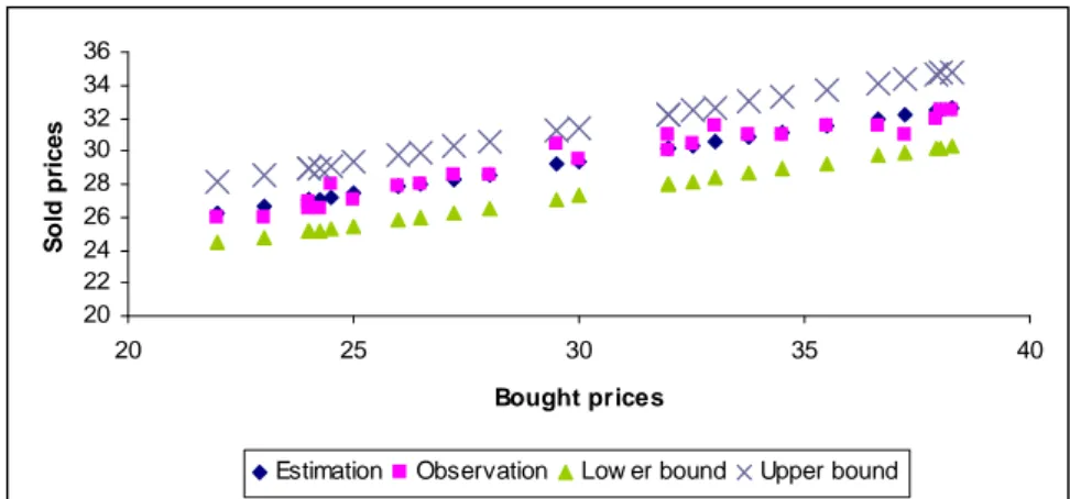
In part of numerical practise data was obtained using bought and sold prices in second hand car business for fuzzy linear regression (http://www.hurriyetoto.com.tr, 01/08/2008). Prices were become fuzzy numbers by describing lower and upper bounds. Data using in the study is prices of 25 cars whose models are 2006 and have the features that Renault Megane Saloon car Diesel 1.5 Dynamical. YTL prices were used dividing by 1000 in order that algorithm can be tried smoothly. Parameter of regularization was accepted 1. Application of based on LS-SVM nonlinear fuzzy regression was practised with an algorithm prepared on Selcuk STAT. Figure 1 shows estimation and estimation interval of observations.
20 22 24 26 28 30 32 34 36 20 25 30 35 40 Bought prices So ld p ri c e s
Estimation Observation Low er bound Upper bound
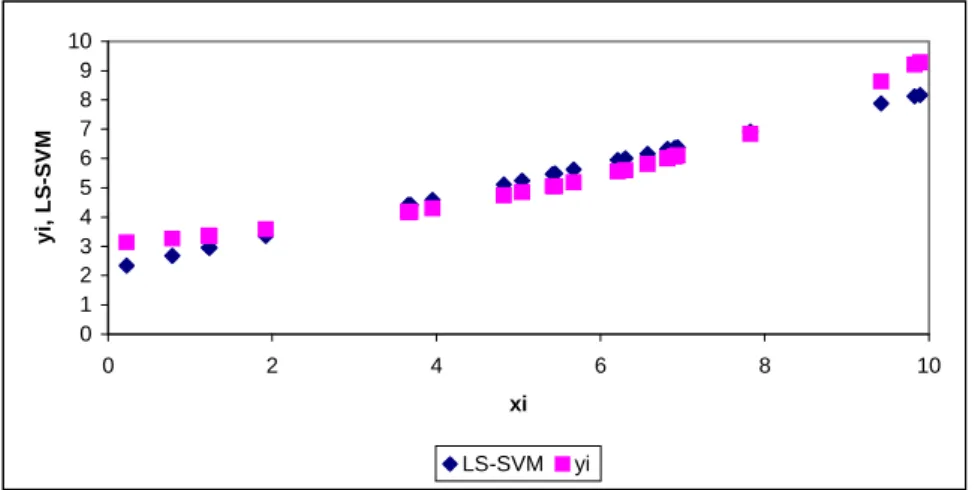
So as to examining productivity of the algorithm of based on LS-SVM fuzzy nonlinear regression independent variables xi were generated from [0.0, 10] with uniform distribution. The spreads of xi were also generated from [0, 1] with uniform distribution.
Dependent variable was occured by
yi = 2.1 + exp(0.2xi) + εi Here εi ~N (0, 0.01) and i = 1, .., 25.
Selcuk STAT was used for practise of LS-SVM. As is seen from Figure 2 prepar-ing model is suitable for fuzzy input and fuzzy output of nonlinear regression.
0 1 2 3 4 5 6 7 8 9 10 0 2 4 6 8 10 xi yi , L S -SV M LS-SVM yi
Figure 2. Estimation values of nonlinear regression
The spreads of estimation values are given at Figure 3. Sum squares of error is 6.289. 0 2 4 6 8 10 12 14 16 0 2 4 6 8 10 xi yi , L S -S V M yi LS-SVM LS-SVM low er LS-SVM upper
5. Results
In this study, an estimation method is obtained for based on LS-SVM fuzzy nonlinear regression. There are some methods for fuzzy nonlinear regression, however, prepared algorithm is independent from a model. Therefore it does not depend on any modelling assumption and suitable for fuzzy nonlinear regression whose input and output are fuzzy. The algorithm wieldy because it depends on operating of matrix inversion.
In numerical example, it can be seen center points of sold prices and their estimates are close. User can constitute lower and upper bounds for sold prices and see getting profit (loss).
In nonlinear example, estimation values are compatible with observation values and the interval with obtaining LS-SVM covers estimation values.
References
1. Dubois, D., Prade, H.(1980): Fuzzy Sets and Systems: Theory and Applications, (New York: Academic).
2. Genc, A.(1997): Multivariate nonlinear models: Parameter Estimation and Testing Hypothesis, Ankara University Institute of Science Doctoral Thesis, Ankara.
3. Hong, D.H., Hwang, C.(2006): Fuzzy Nonlinear Regression Model Based on LS-SVM in Feature Space, FSKD 2006, LNAI 4223, 208-216.
4. Ishibuchi, H., Tanaka, H.(1992): Fuzzy Regression Analysis Using Neural Networks: Fuzzy Sets and Systems, Vol.50, No.3, 257-266.
5. Pedrycz, W., Gomido, F.(1998): An introduction to fuzzy sets analysis and design, (The MIT Press, USA).
6. Polat, G., Altun, H.(2007): Determining Efficiency of Speech Feature Groups in Emotion Detection, IEEE 15. Signal Processing and Communicaiton Applications Congress, SIU 2007, Eskisehir.
7. Sun, Z., Sun, Y.(2003): Fuzzy Support Vector Machine for Regression Estimation, IEEE International Conference on, Vol. 4, 3336 — 3341.
8. Suykens, J., Gestel, T., Brabanter, J., DeMoor, B., Vandewalle, J.(2002): Least Squares Support Vector Machines, (World Scientific Publishing Co. Pte. Ltd., Lon-don).
9. Tanaka, H., Uejima, S., Asai, K.(1982): Linear Regression Analysis with Fuzzy Model, IEEE Transactions on Systems, Man and Cybernetics, Vol. SMC-12, No.6. 10. Teksen, U.M.(2008): Estimation in Fuzzy Nonlinear Regression, Unpublished Post-graduate Thesis, Selcuk University Institute of Science, Konya.
11. Xu, Z., Khosgoftaar, T.M.(2000): Prediction of Software Faults Using Fuzzy Non-linear Regression Modeling, Fifth IEEE International Symposim on. HASE 2000 Vol-ume , Issue, 281 — 290.