An application based on zero-inflated poisson and negative binomial regression models

T.C.

SELÇUK ÜNİVERSİTESİ FEN BİLİMLERİ ENSTİTÜSÜ

SELCUK UNIVERSITY

GRADUATE SCHOOL OF NATURAL SCIENCES

An Application Based on Zero-Inflated Poisson and Negative Binomial Regression Models

Mohamad ALNAKAWA

MASTER of SCIENCE (M.Sc.) THESIS Statistics Department

Supervisor: Assoc.Prof.Dr. Neslihan İYİT

May-2020 KONYA Her Hakkı Saklı

ÖZET

YÜKSEK LİSANS TEZİ

Sıfır Değer Ağırlıklı Poisson ve Negatif Binom Regresyon Modelleri Üzerine Bir Uygulama

Mohamad ALNAKAWA

Selçuk Üniversitesi Fen Bilimleri Enstitüsü İSTATİSTİK Anabilim Dalı

Danışman: Doç.Dr. Neslihan İYİT 2020, 149 Sayfa

Jüri

Danışman: Doç.Dr. Neslihan İYİT Prof.Dr. Aşır GENÇ

Dr. Öğr.Üyesi Yunus AKDOĞAN

Genelleştirilmiş doğrusal modellerde (GLM), bağımlı değişkenin dağılımının üstel aileden geldiği kabul edilmektedir. GLM’de bağımlı değişkenin dağılımı; üstel ailenin yanı sıra, sıfır değer ağırlıklı Poisson ve Negatif Binom dağılımlarından da gelebilmektedir. Bu tez çalışmasında, GLM yapısı hakkında genel bilgiler verildikten sonra, GLM’in özel hali olan Poisson ve Negatif Binom Regresyon Modelleri, model kurma süreçleri ve parametre tahminleri olmak üzere tanıtılmıştır. Daha sonra Sıfır Değer Ağırlıklı Regresyon Modellerinden Sıfır Değer Ağırlıklı Poisson (ZIP) ve Sıfır Değer Ağırlıklı Negatif Binom (ZINB) Regresyon Modelleri detaylı olarak verilmiştir.

Tez çalışmasının orijinal kısmını teşkil eden uygulama aşamasında, Cameron, Congo, Sudan, Vietnam, Pakistan (Punjab region), Pakistan (Sindh region), Zimbabwe, Kyrgyzstan, El Salvador and Mongolia olmak üzere düşük-orta gelirli ülkeler için, 2014 yılında UNICEF tarafından yapılan “Çoklu Göstergeler Küme Araştırması 5” (MICS5) kullanılarak, 5-yaş altı çocuk ölümlerini etkileyen olası risk faktörleri GLM sınıfında yer alan Poisson, Negatif Binom, ZIP ve ZINB Regresyon Modelleri kullanılarak belirlenmeye çalışılmıştır.

Bu amaç doğrultusunda, eğitim (bir okula devam ettiği veya etmediği), servet endeksi beşlisi (en yoksul, ikinci, orta, dördüncü ve en zengin nüfus servet beşlisi), ikamet alanı (kırsal veya

kentsel), annenin yaşı (15-19, 20-24, 25-29, 30-34, 35-39, 40-44, 45-49 yaş), emzirme durumu (anne sütü aldığı veya almadığı) ve doğum kontrol yöntemi (gebeliği önleyici bir yöntem kullandığı veya kullanmadığı) “5-yaş altı çocuk ölümlerini” etkileyen olası risk faktörleri kategorik bağımsız değişkenler olmak üzere alınarak GLM’ler yapılandırılmıştır.

Böylece bu tez çalışmasında ele alınan ülkelerin sosyo-ekonomik ve demografik özellikleri göz önünde bulundurularak, R-programı aracılığıyla, GLM sınıfının özel durumları olan Poisson, Negatif Binom, ZIP ve ZINB Regresyon Modelleri, düşük-orta gelirli ülkeler için 5-yaş altı çocuk ölümleri ile olası risk faktörleri arasındaki istatistiksel bağıntıları modellemek için, AIC, BIC ve AICC olmak üzere bilgi kriterleri ve log-olabilirlik değerleri kullanılarak, karşılaştırmalı olarak incelenmiştir.

Anahtar Kelimeler: Genelleştirilmiş doğrusal model - Sığır-değer ağırlıklı Poisson regresyon modeli - Sığır-değer ağırlıklı Negatif binom regresyon modeli –UNICEF- Çoklu Göstergeler Küme Araştırması - Beş yaş altı çocuk ölümü - Düşük orta gelirli ülkeler.

ABSTRACT MSc. THESIS

An Application Based on Zero-Inflated Poisson and Negative Binomial Regression Models

Mohamad ALNAKAWA

THE GRADUATE SCHOOL OF NATURAL AND APPLIED SCIENCE OF SELCUK UNIVERSITY IN PARTIAL FULFILLMENT OF THE REQUIREMENTS FOR THE DEGREE OF MASTER OF SCIENCE IN

STATISTICS

Supervisor: Assoc.Prof.Dr. Neslihan İYİT 2020, 149 Pages

Jury

Supervisor: Assoc.Prof.Dr. Neslihan İYİT Prof.Dr. Aşır GENÇ

Assist.Prof.Dr. Yunus AKDOĞAN

In generalized linear models (GLM), the distribution of the response variable is considered to come from the exponential family. In GLM, besides the exponential family, the distribution of the response variable can also come from a zero-inflated Poisson and Negative-Binomial distributions. In this thesis study, after general information about GLM structure is given, Poisson and Negative Binomial Regression Models, which are the special cases of GLM, are introduced as in terms of model building processes and parameter estimates. Then, Zero-Inflated Poisson (ZIP) and Zero-Zero-Inflated Negative Binomial (ZINB) Regression Models are given in detail.

The goal of this study is to determine the possible risk factors affecting “child mortality under-5” in some lower middle-income countries such as Cameron, Congo, Sudan, Vietnam, Pakistan (Punjab region), Pakistan (Sindh region), Zimbabwe, Kyrgyzstan, El Salvador and Mongolia by using the “Multiple Indicators Cluster Survey 5 (MICS5)” conducted by UNICEF in 2014, by using Poisson regression model, negative binomial (NB2) regression model, zero-inflated Poisson (ZIP) regression model and zero-inflated negative binomial (ZINB) regression model in the class of generalized linear models (GLMs).

For this purpose, education (as attended to a school or not attended to a school), wealth index quintile (as poorest, second, middle, fourth and richest population wealth quintiles), area of

residence (as rural or urban), mother's age (as 15-19, 20-24, 25-29, 30-34, 35-39, 40-44, 45-49 years), breastfeeding status (as received breast milk or not received breast milk) and pregnancy method (as used any methods to avoid pregnancy or not) are taken as categorical independent variables as possible risk factors affecting “child mortality under-5”.

Thus, considering the socio-economic and demographic characteristics of the countries discussed in this thesis study, Poisson, Negative Binomial, ZIP and ZINB Regression Models, which are the special cases of GLMs class, are used to model the statistical significant relationships between the “child mortality under-5” and the possible risk factors for the lower-middle income countries. These GLMs are compared by using AIC, BIC, AICC as IC and log-likelihood values.

Key Words: Generalized linear model - inflated Poisson regression model - zero-inflated negative binomial regression model – UNICEF - Multiple Indicators Cluster Survey - child mortality under-5 - lower middle-income countries.

ACKNOWLEDGEMENTS

I am eternally grateful to Allah Almighty, who gave me the ability to complete my M.Sc. thesis.

Many thanks to my Mother, Father, Brothers, my family and my friends for their inspiration, guidance and encouragements.

I gratefully acknowledge the great encouragement and full support of my marvelous supervisor “Assoc.Prof.Dr. Neslihan İYİT”. Her guidance helped me in all the time during my M.Sc. study.

I am using this opportunity to express my gratitude to my honorable M.Sc. thesis juries as Prof.Dr. Aşır GENÇ, Assist.Prof.Dr. Yunus AKDOĞAN who supported me throughout the defense of this thesis. And also I am thankful for their advice and guidance to Prof.Dr. Coşkun KUŞ, Prof.Dr. İsmail KINACI, Prof.Dr. M. Fedai KAYA and all my statistics department during my M.Sc. thesis study. With my appreciation and sincerely grateful…

Mohamad ALNAKAWA KONYA-2020

THE CONTENTS

ÖZET ... 1

ABSTRACT ... 3

ACKNOWLEDGEMENTS ... 5

THE CONTENTS ... 6

SYMBOLS AND ABBREVIATION ... 8

LIST OF TABLES ... 10

LIST OF FIGURES ... 14

1.INTRODUCTION ... 15

2. LITERATURE REVIEWS ... 16

2.1. LITERATURE REVIEWS ABOUT ZERO-INFLATED REGRESSION MODELS ... 16

2.2. LITERATURE REVIEWS ABOUT CHILD MORTALITY UNDER-5 ... 17

3. GENERALIZED LINEAR MODELS ... 19

3.1. The Structure of Generalized Linear Models ... 19

3.1.1. The Random Component ... 19

3.1.2. The Systematic Component (The Linear Predictor) ... 21

3.1.3. The Link Function ... 21

4. BUILDING POISSON REGRESSION MODEL ... 22

4.1. Usage of the Poisson Distribution ... 23

4.2. Poisson Regression Model Assumptions ... 23

4.3. Poisson Regression Model ... 24

4.4. Buılding Stage of Poisson Regression Model ... 24

4.5. Parameter Estimation of Poisson Regression Model ... 25

5. BUILDING NEGATIVE-BINOMIAL REGRESSION MODEL ... 26

5.1. Negative-Binomial Regression Model Assumptions ... 27

5.2. Negative-Binomial Regression Model ... 27

5.3. Parameter Estimation of Negative-Binomial Regression Model ... 29

6. ZERO-INFLATED REGRESSION MODELS ... 31

6.2. Zero-inflated Negative Binomial Regression model ... 34

6.3. Evaluation of the Goodness-of-Fit of the Generalized Linear Models ... 36

7. APPLICATIONS OF GENERALIZED LINEAR MODELS TO THE CHILD MORTALITY UNDER-5 DATA IN SOME LOWER–MIDDLE INCOME COUNTRIES ... 38

7.1 Generalized Linear Model Analysis to the Child Mortality Under-5 Data in Some Lower Middle-Income Countries ... 47

7.2 Results and discussion ... 119

8. CONCLUSION AND RECOMMENDATION ... 145

8.1 Conclusion ... 145

8.2 Recommendation ... 147

REFERENCES ... 148

SYMBOLS AND ABBREVIATION ABBREVIATION

AIC: Akaike Information Criterion.

AICc: Corrected Akaike Information Criterion. BIC: Bayesian Information Criterion.

CDEAD : The Number of Deaths of Children Under-5. EU: European Union.

GLMs: Generalized Linear Models.

GP: Generalized Poisson Regression Model. HIV : Human Immunodeficiency Virus. MICS: Multiple Indicators Cluster Survey. NBR: Negative Binomial Regression Model.

PR: Poisson Regression Model. R: R-Programming.

TDHS: Turkey Demographic and Health Survey. UN : United Nations.

U-5 : Under five years old child. WAGE : Mother's Age.

WHO : World Health Organization.

UNICEF : United Nations International Children's Emergency Fund ZIGP: Zero-inflated Generalized Poisson Regression Model.

ZINB:Zero-inflated Negative Binomial Regression Model.

SYMBOLS

a(.),b(.),c(.) : known functions.

E(Y) : expected value of response variable.

qi: canonical parameter. f :dispersion parameter. ei : random errors. , i i x z : explanatory variables. h_i : linear predictor. g(.) :link function. L: log-likelihood function. l

g( ): canonical link function. SE :standard error.

bi, gi: Regression parameters.

Var(Y): variance of response variable. N: sample size.

LIST OF TABLES

Table 3.1.Some common link functions used in the GLM ... 22

Table 6.1. ZIP, ZINB ,Poisson and NB regression models with expectation and variance values. ... 36

Table 6.2. Some Information criteria for choosing the best GLM. ... 38

Table 7.1. List of countries used in the study. ... 39

Table 7.2. Description of the variables used in the data analysis. ... 40

Table 7.3. Perecentages for the mortality of children under-5. ... 41

Table 7.4. Percentages for the education (attended to a school or hadn't attended to a school) of the mother. ... 42

Table 7.5. Percentages for the wealth index quantiles of the family. ... 43

Table 7.6. Percentages for the mother's age. ... 44

Table 7.7. Percentages for the area of residence (rural or urban). ... 45

Table 7.8. perecentages for pregnancy method (used any method or not). ... 46

Table 7.9. Percentages for the mother’s breastfeeding status (received breast milk or not). ... 47

Table 7.10. Results of Poisson regression model. ... 48

Table 7.11. Results of Negative Binomial regression model. ... 50

Table 7.12. Results of Zero–inflated Poisson regression model. ... 52

Table 7.13. Results of Zero-inflated Negative Binomial model. ... 54

Table 7.14. Results of Poisson regression model for Cameron country data. ... 56

Table 7.15. Results of Negative Binomial regression model for Cameron data.. ... 58

Table 7.16. Results of Zero–inflated Poisson regression model for Cameron data ... 60

Table 7.17. Results of Zero–inflated Negative-Binomial regression model for Cameron data ... 61

Table 7.18. Results of Poisson regression model for Cameron data. ... 63

Table 7.19. Results of Negative Binomial regression model for Cameron data. ... 64

Table 7.21. Results of Zero-inflated Negative Binomial regression model for Congo

data. ... 67

Table 7.22. Results of Poisson regression model for El Salvador data. ... 69

Table.7.23. Results of Negative Binomial regression model for El Salvador data. ... 70

Table 7.24. Results of Zero–inflated Poisson regression model for El Salvador data. . 72

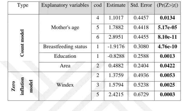
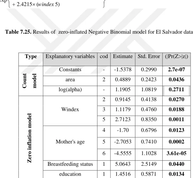
Table 7.25. Results of Zero-inflated Negative Binomial regression model for El Salvador data. ... 73

Table 7.26. Results of Poisson regression model for Kyrgyzstan data. ... 75

Table 7.27.Results of Negative Binomial regression model for Kyrgyzstan data. ... 76

Table 7.28. Results of Zero–inflated Poisson regression model for Kyrgyzstan data. .. 77

Table 7.29. Results of Zero-inflated Negative Binomial regression model for Kyrgyzstan data. ... 78

Table 7.30. Results of Poisson regression model for Mongolia data. ... 80

Table 7.31. Results of Negative Binomial regression model for Mongolia data. ... 81

Table 7.32. Results of Zero–inflated Poisson regression model for Mongolia data. ... 83

Table 7.33.Results of Zero-inflated Negative Binomial regression model for Mongolia data. ... 84

Table 7.34. Results of Poisson regression model for Punjab region data. ... 86

Table 7.35. Results of Negative Binomial regression model for Punjab region data. .... 87

Table 7.36. Results of Zero–inflated Poisson regression model for Punjab region data. ... 89

Table 7.37. Results of Zero-inflated Negative Binomial regression model for Punjab region data. ... 91

Table 7.38. Results of Poisson regression model for Sindh region data. ... 93

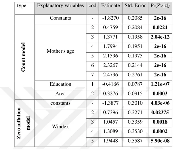
Table 7.39. Results of Negative Binomial regression model for Sindh region data. ... 94

Table 7.40. Results of Zero–inflated Poisson regression model for Sindh region data. 96 Table 7.41. Results of Zero-inflated Negative Binomial regression model for Sindh region data. ... 98

Table 7.42. Results of Poisson regression model for Sudan data. ... 100

Table 7.44. Results of Zero–inflated Poisson regression model for Sudan data. ... 103 Table 7.45. Results of Zero-inflated Negative Binomial regression model for Sudan data. ... 105 Table 7.46. Results of Poisson regression model for Vietnam data. ... 107 Table 7.47. Results of Negative Binomial regression model for Vietnam data. ... 108 Table 7.48. Results of Zero–inflated Poisson regression model for Vietnam data. .... 109 Table 7.49. Results of Zero-inflated Negative Binomial regression model for Vietnam data. ... 110 Table 7.50. Results of Poisson regression model for Zimbabwe data. ... 112 Table 7.51. Results of Negative Binomial regression model for Zimbabwe data. ... 113 Table 7.52. Results of Zero–inflated Poisson regression model for Zimbabwe data. . 115 Table 7.53. Results of Zero-inflated Negative Binomial regression model for

Zimbabwe data. ... 117 Table 7.54. Using information criteria to compare GLMs for choosing the best model for overall child mortality under-5 data ... 119 Table 7.55. Using information criteria to compare GLMs for choosing the best model for Cameron child mortality under-5 data. ... 121 Table 7.56. Using information criteria to compare GLMs for choosing the best model for Congo child mortality under-5 data ... 123 Table 7.57. Using information criteria to compare GLMs for choosing the best model for El-Salvador child mortality under-5 data ... 125 Table 7.58. Using information criteria to compare GLMs for choosing the best model for Kyrgyzstan child mortality under-5 data. ... 126 Table 7.59. Using information criteria to compare GLMs for choosing the best model for Mongolia child mortality under-5 data ... 129 Table 7.60. Using information criteria to compare GLMs for choosing the best model for Pakistan –Punjab child mortality under-5 data. ... 131 Table 7.61. Using information criteria to compare GLMs for choosing the best model for Pakistan –Sindh child mortality under-5 data. ... 132 Table 7.62. Using information criteria to compare GLMs for choosing the best model for Sudan child mortality under-5 data. ... 134 Table 7.63. Using information criteria to compare GLMs for choosing the best model for Vietnam child mortality under-5 data ... 136

Table 7.64. Using information criteria to compare between GLMs and choose the best model for Zimbabwe data. ... 138

LIST OF FIGURES

Figure 1.1.Special count models in GLMs when the dependent variable is count data..16

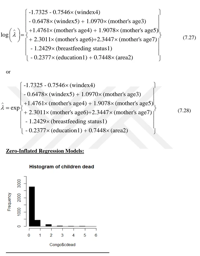
Figure 7.1. Histogram of mortality children under five years for collection data. ... 51

Figure 7.2. Histogram of mortality children under five years for Cameron data……...65

Figure 7.3. Histogram of mortality children under five years for Congo data. ... 65

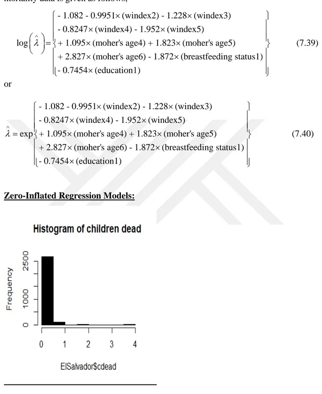
Figure 7.3. Histogram of mortality children under five years for El Salvador data. ... 71

Figure 7.4. Histogram of mortality children under five years for Kyrgyzstan data. ... 77

Figure 7.5. Histogram of mortality children under five years for Mongolia data. ... 82

Figure 7.6. Histogram of mortality children under five years for Punjab data. ... 88

Figure 7.7. Histogram of mortality children under five years for Sindh data. ... 95

Figure 7.8. Histogram of mortality children under five years for Sudan data. ... 102

Figure 7.9. Histogram of mortality children under five years for Vietnam data. ... 108

1.INTRODUCTION

Regression analysis has been used as one of the most popular statistical techniques for centuries to build the statistically significant relationships between independent and dependent variables and also it is used to estimate or forecast the values of dependent variable in the aspect of independent variables. Traditional regression analysis consists of simple linear regression for one independent variable and multiple linear regression model for more than one independent variables (Montgomery et al., 2012).

As a general case, in the multiple linear regression model given below;

b b b b e

= 0 + 1 1 + 2 2 +...+ +

i i i i

y x x x (1.1)

where: i= 1,2,...,n, y_i is the dependent variable,(x₁,x₂, ...,xi)are the independent variables,(b b₁, ₂...b_i) are the partial regression coefficients for the independent variables, and also b is the constant value expresses the mean (average) 0

value of the dependent variable when all independent variables are equal to zero,

and also ei is the random error term assumed to be normally distributed with mean zero and the constant variance s2 as _{~ (0,} 2₎

i N

e s (Olsson, 2002; Montgomery et al., 2012).

Generalized linear model (GLM) is a generalization of the linear model when the dependent variable follows different distributions besides the normal distribution belonging to the exponential family such as Poisson Distribution, Gamma Distribution, inverse Gaussian Distribution, Negative Binomial Distribution and etc.). When too many zeros are observed in the structure of the dependent variable, it is called overdispersion. In this special situation, zero-inflated Poisson (ZIP) regression model and zero-inflated Negative Binomial (ZINB) regression model are used as special cases of GLMs called as zero-inflated regression models(Fox, 2015).

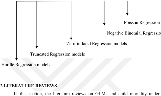
When the dependent variable is binary, logistic regression model and log-linear model can be used as special cases of GLMs. When the dependent variable is count data, count models given in Figure 1.1 can be used as exciting special cases of GLMs to

discover more than zero-inflated Poisson and Negative Binomial regression models(Olsson, 2002; Fox, 2015).

Figure 1.1.Special count models in GLMs when the dependent variable is count data

Poisson Regression Negative Binomial Regression

Zero-inflated Regression models

Truncated Regression models

Hurdle Regression models

2.LITERATURE REVIEWS

In this section, the literature reviews on GLMs and child mortality under-5 concepts are given in details.

2.1. Literature Reviews about Zero-inflated Regression Models

Karaca and Olmuş (2018) studied Poisson, negative binomial, zero-inflated Poisson and zero-inflated Negative Binomial regression models to study the factors affecting customer service in the service sector. The independent variables are the number of complaints received from the customers and also customers’ gender, age, education and experience.

Yeşilova et al. (2012) investigated e-mail traffic at the University of Yüzüncü Yıl based on a questionnaire answered by 1163 university staff, including 568 academicians, and 595 administrative staff as internet server reviews. Because of the large number of zeros in this survey data, among inflated Poisson (ZIP), zero-inflated negative binomial (ZINB), Poisson Hurdle and negative binomial Hurdle regression models, ZINB was selected as the best GLM acoording to the AIC information criteria for the data analysis.

Mouatassim and Ezzahid (2012) applied Poisson and generalized Poisson regression models to analyze private health insurance data in the aspect of age, gender,

marital status and etc. as the independent variables. By using Vuong's test, these models are compared and ZIP regression model performed better than the other GLMs.

Bodromurti et al. (2018) studied ZINB regression model to determine the factors affecting the number of infant mortality in Indonesia as the dependent variable and the mother's education level, age, region and etc. as the independent variables.

Evans and Adenomon (2014) analyzed the General Hospital’s malaria data to determine the factors affecting the spread of malaria in the state of Mina, Nigeria by using negative binomial and Poisson regression models.

Oritogun et al. (2018) analyzed Nigerian health and demographic survey data in 2008 to reduce the child mortality rate by using the Poisson, ZIP, Negative Binomial (NB), and ZINB regression models. As a result of this study, Poisson and ZINB regression models are better performed than the other GLMs according to AIC information criteria and Lilliefors test to determine the factors affecting child mortality in the aspect of level of the parental education, family planning and healthy nutrition.

Yanikkaya and Selim (2010) investigated the mortality rates of children in the western and southern regions of Turkey based on the Turkish Population and Health Survey (TDHS) data from 1998 to 2003 by using NB regression model. The number of children deaths is taken as the dependent variable, the region, mother’s and father’s education level, mother’s age at the first birth, whether contraception is used or not, the economic situation, assets of parents are Turkish or not, the duration of marriage and etc. are taken as the independent variables.

Ismail and Zamani (2013) explained the relationships between the NB, ZINB and the generalized Poisson (GP) regression models including an application based on the evidence of the German health team and another application based on the data car insurance in Malaysia from 2001 to 2003.

2.2. Literature Reviews about Child Mortality Under-5

Sengoelge et al. (2011) emphasized the most important causes of child mortality under-5 in European (EU) countries such as fatal home injuries, drowning, poisoning, suicide and killing and calculated injury mortality rate for 16 EU countries between 2002 and 2004.

Taha et al. (2000) examined HIV-infected children morbidity and mortality by using Kaplan-Meier analyses and proportional hazards models to estimate the survival of these children.

Ali and Shah (2000) estimated maternal and child mortality under-5 in the south/centre of Iraq in 1999 after Gulf Conflict and founded that child mortality under-5 born from women with no education was higher in rural areas.

Abou-Ali (2003) indicated the importance of environmental and educational problems on the infant and child mortality rate in Egypt and improving municipal services related to drinking water and sanitation, hygiene and also high level of education contribute to reducing child mortality.

Bartlett and Planning (2002) studied the factors affecting child disability, mortality and morbidity in developing countries especially in low-income countries such as unsuitable living conditions, traffic accidents, lack of safe play places and inadequate child care.

Kerkeni et al. (2007) aimed to evaluate the social status, prevalence of consanguineous marriages and the effects of relatives on reproductive behavior on child mortality in Tunisia.

Farah et al. (1982) compared child mortality in Sudan in two samples including the first sample from the census of 1973 in Sudan and the second sample from the city of Khartoum in the aspect of father’s occupation, woman’s place of birth, education, characteristics about marriage and etc.

This study consists of six main sections. In Sections 1 and 2, introduction and literature reviews about zero-inflated regression models and child mortality under-5 are given. Theoretical knowledges are given in Sections 3, 4 and 5. In Section 3, generalized linear models (GLMs) is introduced and in Sections 4 ,5 and 6 information about Poisson regression and negative binomial regression are given.

In Section 7, zero-inflated regression models as zero-inflated Poisson regression model and zero-inflated negative binomial regression model are briefly investigated. Section 7 includes the practical section consisting of the statistical modeling of child mortality under-5 data provided by UNICEF Multiple Indicator Clusters (MICS 5) Survey in the selected lower middle-income countries, depending on the World Bank's 2019 ranking.

using the models mentioned in the theoretical section, estimating the coefficients of regression models using the R programming language, comparing the models using several criteria (AIC,BIC,loglikelihood and etc)and choosing the best model.

3.GENERALIZED LINEAR MODELS (GLMs)

Generalized linear model concept was first introduced by (Nelder and Wedderburn, 1972). In the following years, many researchers continued to work on GLM such as(Altland, 1999; McCulloch, 2000; Olsson, 2002; Winkelmann, 2008; Agresti, 2010; Madsen and Thyregod, 2010; Hilbe, 2011; Fox, 2015).

3.1.The Structure of Generalized Linear Models

There are 3 parts in GLMs as the random component, the systematic component and the link function.

3.1.1 The random component

The distribution of the response variable comes from the exponential family such as Poisson, Negative Binomial, gamma, exponential and etc. and also the response variable may come from zero-inflated distributions other than the exponential family (Fox, 2015).

The exponential family including many known distributions can be written as follows (Olsson, 2002; Fox, 2015);

(

( ))

( ; , )

exp

( , )

( )

y

b

f y

c y

a

q

q

q f

f

f

é

_-

ù

ê

ú

=

_ê

+

_ú

ë

û

(3.1)

where

a

(.), (.), (.)

b

c

are known functions,

q

is the canonical parameter indicating the location of the distribution, f is the dispersion parameter indicating the scale of the distribution.

The expected value and the variance of the response variable having a special distribution coming from the exponential family can be written as follows;

( )= '_{( )}q

E Y b (3.2)

''

( )

( ). ( )

Var Y

=

a

f

b

q

(3.3)

Proof of the Eq.(3.2)(Olsson, 2002)

Step 1. Let's denote the log-likelihood function of the parameters for the exponential family as follows;

q f = q f

( , ; ) log ( ; , )

Lf y f y (3.4) Step 2. Let's write the following relationships of the expected values according to the likelihood theory q q æ¶ ö_÷ ç _÷= ç _÷ çè ¶ ø log ( ; ) 0 f y E (3.5) q q q q æ¶ ö_÷ æ¶ ö ç _÷+ ç ÷_{÷ =} ç _÷÷ ç_{ç ÷} ç ¶ è ¶ ø è ø 2 2 2 log ( ; )f y log ( ; )f y ₀ E E (3.6)

Step 3. Log-likelihood of the exponential family can be written as follows;

q f q q f f -= ( )+ log ( ; , ) ( , ) ( ) y b f y c y a (3.7)

q f

q

q

f

¶

₌

-¶

'

log ( ; , )

( )

( )

f y

y b

a

(3.8) q f q q f ¶ -= = ¶ ' log ( ; , ) ( ) ( ) ( ) 0 ( ) f y y b E E a _(3.9)

q

(

q

)

f

f

-

'

₌

_-

₌

'

( )

1

(

)

( )

( )

0

( )

( )

y b

E

E Y

b

a

a

(3.10) E Y( )=b'( )q

Proof of the Eq.(3.2)(Olsson, 2002) 2 ''

_{( )}

'

_{( )}

0

( )

( )

b

y

b

E

E

a

a

q

q

f

f

æ

ö

æ

ö

_÷

_ç

æ

_-

ö

_÷

_÷

ç

_-

_÷

₊

_ç

ç

_÷

÷

₌

ç

_÷

_ç

ç

_{÷ ÷}

÷

ç

÷

ç

÷

ç

ç

ç

_÷

è

ø

_çè

è

ø

_ø

(3.11) q _q f f - ''( )+ 1 ₍ - '_{( ))}2 =₀ ( ) ( ) b E Y b a a (3.12)

On the other hand, Var Y( )=E Y( ) ( ( ))- E Y 2 (3.13) q f f - ''( )+ 1 ₍ - _{( ))}2 = ₀ ( ) ( ) b E Y E Y a a (3.14) Var Y( )=a( ). ( )f b'' q

3.1.2.The systematic component (the linear predictor)

The systematic component is the set of independent variables and the unknown parameters which are defined as follows(Altland, 1999; Freund et al., 2006);

hi =b0 +b1xi1+...+bk ikx (3.15)

3.1.3. The link function

The main purpose of the GLM to develop a linear model for an appropriate function of the expected value of the dependent variable is to build a link function (Montgomery et al., 2012). Therefore, the link function is the function that establishes the relationship between the expected value of the dependent variable and the linear predictor. Link functions in GLM are specific to the distributions of the response variable. Each of the distributions from the exponential family has a natural link function called the “canonical link” function. The link function g(.) that transposes the expected value of response variable into a linear predictor can be given as follows;

l =h =b0 +b1 1+ +b

and the inverse link function g−1

( )

. that transposes the expected value of response variable into a linear predictor can be given as follows;

l ₌ -1 l ₌ -1 b ₊b _{+ +}b

0 1 1

( ) ( ... )

i g i g xi k ikx (3.17) where

g

-1

( )

l

_i is called the mean function(Olsson, 2002; De Jong and Heller, 2008; Fox, 2015).

Table 3.1.Some common link functions used in the GLM (McCulloch, 2000; Olsson, 2002; Fox, 2015)

Link function Canonical link function Invers link function

identity _{h= ( )g l l =g}-1_{( )h} invers l-1 _h-1 logistic l l -log 1 + h 1 1 e log

log( )l

el

4.BUILDING POISSON REGRESSION MODEL

Poisson distribution was named after the French mathematical Sim´eon Denis Poisson (1781–1840) and was first published in 1837.

The Poisson distribution is a probability distribution of a discrete random variable that indicates the number of the events independent of each other that occurs during a given unit of time or space.

The Poisson distribution is defined as follows (Walck, 1996);

( , ) ! i yi i i i i e P y y l_l l = - (4.1)

where l is the parameter of the Poisson distribution, y is the random variable taking values 0,1,2,3,….The expected value and the variance of the response variable having Poisson distribution can be written as follows (Walck, 1996; Letkowski, 2012);

( )

i

( )

i i

E Y =Var Y =λ (4.2)

Proof of the Eq. (4.2)

By using the general formula of the exponential family given in Eq.(3.1), the expected value and the variance of the response variable having Poisson Distribution can be calculated as follows (Hilbe, 2011);

l l

=

-log ( )f yi yi log i i log( !)yi (4.5)

{

l l

}

=

-( )_i exp _ilog _{i i} log( !)_i

f y y y (4.6) f = q = l q =l ( ) 1, _i log , ( )_{i i i} a b (4.7) q _l q ¶ = = ¶ ( ) ( ) i i i i b E Y q f l q ¶ = = ¶ 2 2 ( ) ( ) ( ) i i i i b V Y a

4.1. Usage of the Poisson distribution

The Poisson Distribution plays an important and significant role in many fields and applications as mentioned below;

1-It is often used in the field of banks. For example; number of the banks that went bankrupt during a month (Letkowski, 2012).

2- It is often used in field of technology. For example; the number of the number of arrivals at a car wash during a time unit (Anderson et al., 2020).

3- It is often used for the rare events. For example; the number of a certain type of insect that can be found in a certain area of the agricultural land(Pelosi and Sandifer, 2003).

4.2.Poisson regression model assumptions

Assumption 1. The conditional probability function of the response variable follows the Poisson distribution with parameter λ (Walck, 1996; Hastings, 1997).

Assumption 2. The Poisson distribution parameter λ for the ith subject equals to the exponential form of the linear predictor as follows (Hilbe, 2011; Fox, 2015) ;

b

l = '

i

x

i e (4.8)

Assumption 3. There is independence between the explanatory and the response variables. By applying the properties of the Poisson distribution to the Poisson regression, the expected value and the variance of the response variable can be written as follows (Winkelmann, 2008); b l = = = ' ( / ) ( / ) i i i _i x E Y X Var Y X e (4.9)

4.3. Poisson Regression Model

The Poisson regression model is one of the models used to analyze the count data. The Poisson regression model is also called as the log-linear model(Deniz, 2005; Winkelmann, 2008).

Let ( , ,....,x x_{i1 i2} x be the values of the independent variables for the _ip) observation i. The Poisson regression model relates the probability of the dependent variable y to the vector of the explanatory variables ( , ,....,x x_{i1 i2} x and it is used to _ip) model the count data where the dependent variable can take nonnegative integers such as 0,1,2,3,…. (Fox, 2015). The Poisson regression model can be written as (Olsson, 2002; Agresti, 2010; Hilbe, 2011);

l =b0 +b1 1 + +b

log( )i xi ... k ikx (4.10)

4.4. Building Poisson regression model

Step 1. Let’s denote the linear predictor part of the GLM as follows(Olsson, 2002; Freund et al., 2006);

h_i =b₀ +b₁x_i1 +...+b_{k ik}x (4.11)

Step 2. Let’s denote the link function g(.) to relate

h

_i to m =_i E Y( )_i in the GLM as follows(Olsson, 2002);

In this case, the link function is called the canonical link function as follows(Olsson, 2002) ;

qi =b0 +b1xi1 +...+bk ikx (4.13)

q_i = log( )l_i ( 4.14)

4.5. Parameter estimation of the Poisson regression model

To estimate the parameters of the Poisson regression model, maximum likelihood (ML) function is used. Let X_i1,X_i2,...,X_in be the explanatory variables. And then the likelihood function of the Poisson regression model parameters can be given as follows (Winkelmann, 2008; Hilbe, 2011; Gupta et al., 2013);

1 ! i i y n i i i e L y l l -= = Õ (4.15) And then by taking the logarithm of the likelihood function given in Eq. (4.15);

( )

{

(

)

( )

}

1

log log i i log !

n y i i i L l e-l y = =

å

- (4.16)

( )

{

( )

( )

( )

}

1

log log i log i log !

n y i i i L l e-l y = =

å

+ - (4.17)

( )

{

( )

( )

}

1

log log log !

n i i i i i L y l l y = =

å

- - (4.18) Log-likelihood function of the Poisson regression model parameters can be given as follows ;

( )

{

_' '

( )

}

1 log log ! n X i i i L y X b e b y = =

å

- - (4.19) Let's take the partial derivatives of the Poisson regression model parameters and then equalizing the log-likelihood function to zero;

( )

_{

_' '

_{( )}

_}

1 log log ! n X i i i L y X b e b y b b = ¶ ¶ = - -¶ ¶

å

(4.20)

( )

_{

_{' '} '

_}

1 log 0 n X i i L y X X e b b = ¶ = - = ¶

å

(4.21) can be found. But the explicit form for the solution of Eq. (4.21) can only be calculated by using iterative methods such as "Newton Raphson and Fisher" by using R programming.

5.BUILDING NEGATIVE-BINOMIAL REGRESSION MODEL

Let's build the negative-binomial (NB) distribution, which is a mixed distribution of Poisson distribution and Gamma distribution, according to the following steps;

Step 1. Let's suppose the

y

_i random variables follow the Poisson distribution with parameter l as follows(Hilbe, 2011; Irungu, 2013);

( ) ! y e f y y l_l -= (5.1) Step 2. Let's suppose lrandom variable follows the Gamma distribution with parameter

a q, as follows(Hilbe, 2011; Irungu, 2013) ; 1

( )

( )

g

e

l q a q

l

l

q a

-=

G

(5.2)

where the expected value and the variance of the response variable can be written as follows ;

( )

E

l

=

aq

(5.3)

( )

2

Var l =aq (5.4)

Step 3. The joint probability distribution of the Poisson and Gamma mixture distributions are as follows ;

1 ( ) ( ) ! ( ) y e f y g e y l l q a q l l l q a -- -= G (5.5)

Step 4. The unconditional distribution also called as the negative binomial distribution (NB) of Y can be written as follows ;

1 0 ( ) ! ( ) y e f y e d y l l q a q l l _l q a ¥ ì_ï - - - ü_ï ï ï = í_ï ý_ï G ï ï î þ

ò

(5.6) ( ) a a q a q q æ ö æ ö G + _{ç ÷ ç ÷} = _{çç ÷÷ çç ÷÷} è ø è ø G G + + + ( ) 1 ( ) ( 1) 1 1 y y f y y (5.7)

The expected value and the variance of the NB distribution are given as follows (Hilbe, 2011);

( )

_i

E Y

=

aq

(5.8) 2

( )

_i

Var Y

=

aq aq

+

(5.9)

5.1. Negative-binomial Regression Model Assumptions

There are many common borrowings between the negative-binomial regression model and the Poisson regression model such as being linear to model parameters, independence of the individual observations (Yang et al., 2015). While the conditional variance of the response variable for the negative binomial distribution allows it to be greater than the conditional mean (Hilbe, 2011).

5.2. Negative-Binomial Regression Model

Negative-binomial regression is used as an alternative method to the Poisson regression.In the negative-binomial regression model, the variance of the response variable takes greater values than its expected value. The parameters of the traditional negative-binomial regression model can be estimated by using the maximum likelihood method as a member of the GLMs (Hilbe, 2002). Negative-binomial regression parameters are taken as l =aq and f 1

a

= ,where l_i > 0 is the mean of response

The negative-binomial regression model can be given as follows (Hilbe, 2011; Zwilling, 2013); f f fl l f f fl fl -æ ö æ ö G + _{ç ÷÷ ç ÷÷} = ç_{çç ÷÷} ç_{çç ÷÷} G G + è + ø è + ø 1 1 1 1 ( ) 1 ( , , ) ( ) ( 1) 1 1 i y i i i i i i i y P y y (5.10)

In the negative-binomial regression model, the mean of the response variable can be written as follows;

l =b0 +b1 1 + +b

log( )i xi ... k ikx (5.11)

where b b b₀, , ,...,_{1 2} b_i are unknown paramters whıch are estimated from data and 1 2

( , ,....,x x_{i i} x_ip)is the vector of the explanatory variables.

The expected value and the variance of the response variable as follows;

l

=

( )

_{i i}

E Y

(5.12)

l

fl

=

+

2

( )

_{i i i}

Var Y

(5.13)

Proof of the Eq.s (5.12) and (5.13) (Hilbe, 2011)

By depending on the definition of the exponential family; 1 1 1

(

)

1

( ; , )

1

1

! (

)

i y i i i i i

y

P y

y

f

f

fl

f l

fl

fl

f

-æ

ö æ

ö

G

+

_ç

_÷

_÷

_ç

_÷

_÷

ç

ç

=

_ç

_÷

_÷

_ç

_÷

_÷

÷

÷

ç

+

ç

+

G

è

ø è

ø

(5.14)

Step 1. Let's take the logarithm of Eq. (5.14);

f fl f l f f fl f ì æ öü ï _÷ï ï _{ç + - ÷}ï ï _{æ ö æ ö} ç_{ç ÷}ï ï _{÷ ÷}ï ï ç ÷ ç _÷ ç ÷ï = _ïí ç_{ç + ÷÷}÷+ _çç_{ç + ÷÷}+ _çç ÷_÷ý_ï è ø è ø ç ÷ ï _{ç - ÷}ï ï ç_ç ÷_÷ï ï _{è ø}ï ï ï î þ 1 ₁ 1 1

( ; , ) exp log log log

1 1 1 ₁ i i i i i i y P y y (5.15)

q q fl q l fl f f = ® = + -log( ) 1 i i i i i i e e (5.16) q fl fl = + 1 i i i e _(5.17) q f fl = -+ 1 1 ( ) log( ) 1 i i b (5.18)

( )

1

a

f =

_(5.19)

Step 3. Let calculate the expected value and the variance of the response variable as follows;

l

f

q

l

f

l

l

q

f

f

¶ ¶

=

=

=

+

=

¶

¶

+

1

( )

'( )

(

). .(1

)

1

i i i i i

b

E Y

b

f

q

l

fl

=

=

+

( )

_i

( ). ''( )

_i

(1

_i

)

Var Y

a

b

5.3. Parameter Estimation of the Negative-Binomial Regression Model

By using the ML method and the assumptions of the GLM, by taking

l

=

( )

i i

E Y

,

Var Y

( )

_i

=

l

_i

+

al

_i2 and

log

( )

l

_i

=

X

'

b

, the likelihood function can be given as follows ( ); l f = = Õ 1 1 ( , , ) n i i i L p y (5.20) f f fl f fl fl -= é _{G + æ ö æ ö} ù ê ç ÷_÷ ç ÷_÷ ú = Õ_êê_{G G +} ç_{èçç + ÷}÷_{ø èçç}ç _{+ ÷}÷_ø ú_ú ë û 1 1 1 1 ( ) 1 ( ) ( 1) 1 1 i y n i i i i i i y L y (5.21)

The log-likelihood function can be given as follows ;

( )

(

)

(

)

fl _fl fl f f f = ì æ ö æ öü ï _{÷ ÷}ï ï ç _{÷ - + + G}ç _{+ ÷}ï ï ç_{ç ÷} ç _÷ï ï _{ç +è} ÷_ø ç_è ÷_øï ï ï ï ï = _{í ý} ï _{æ ö} ï ï _{ç ÷} ï ï- G + - Gç ÷ ï ï _{ç ÷}÷ ï ï è ø ï ï ï î þ

å

1 1 1

log log 1 log

1 log 1 log 1 log i i i i n i i i y y L y (5.22)

( )

(

)

(

)

b b b f f f f f f = ì æ ö ü ï _÷ æ öï ï ç _{÷ - + + G}ç ₊ ÷ï ï ç_ç ÷ ç ÷_÷ï ï _{ç ÷÷} ç_è ÷_øï ï è + ø ï ï ï = í_ï ý_ï æ ö ï _{ç ÷} ï ï_{- G + - Gç ÷} ï ï _{ç ÷}÷ ï ï è ø ï ï ï î þ

å

' ' ' 1 1 1

log log 1 log

1 log 1 log 1 log X X i _X i n i i e y e y e L y (5.23)

Let's take the partial derivatives of the log-likelihood function given by Eq.(5.23) with respect to the parameters and equalizing it to zero;

( )

(

)

(

)

b b b f _f f f b b f f = ì ì æ ö üü ï ï ïï ï ï ç ÷_÷ ïï ï ï ç _÷- + ïï ï ï ç_{ç ÷÷} ïï ï ï + ïï ¶ ₌ ¶ _{ï ï} è ø _ïï= í í ýý ï ï ïï ¶ ¶ _{ïï ïï} æ_ç ö_÷ æ ö_{ç ÷ïïïï} + Gç + ÷- G + - Gç ÷ ï ï _ç ÷_{÷ ç} ÷_÷ïï ï ï è ø è øïï ï ïî ïïþ î þ

å

' ' ' 1 1 log log 1 1 log 0 1 1

log log 1 log

X X i _X n i i i e y e e L y y (5.24) ( )

(

)

(

)

b b b f _f f f f f f f = ì ì æ ö üü ï ï ïï ï ï ç ÷_÷ ïï ï ï ç _÷- + ïï ï ï ç_{ç ÷÷} ïï ï ï + ïï ¶ ₌ ¶ _{ï ï} è ø _ïï= í í ýý ï ï ïï ¶ ¶ _{ïï ïï} æ_ç ö_÷ æ ö_{ç ÷ïïïï} + Gç + ÷- G + - Gç ÷ ï ï _ç ÷_{÷ ç} ÷_÷ïï ï ï è ø è øïï ï ïî ïïþ î þ

å

' ' ' 1 1 log log 1 1 log 0 1 1

log log 1 log

X X i _X n i i i e y e e L y y ( 5.25)

can be found. But the explicit form for the solution of Eq. (5.25) can only be calculated by using iterative methods such as "Newton Raphson and Fisher " by using R programe.

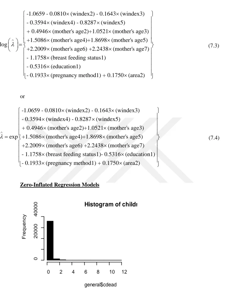
6. ZERO-INFLATED REGRESSION MODELS

Zero-inflated models were first discovered by Lambert in 1992. These models consist of binary model and count model such as zero-inflated Poisson regression model, zero-inflated negative binomial regression model (Hilbe, 2011; Lundy, 2016). These models are used in the following cases;

Case 1: In the count data that contain excess zeros.

Case 2: When the variance of the dependent variable is greater than the expected value the dependent variable, this is called “over-dispersion”.

6.1. Zero-inflated Poisson Regression Model (ZIP)

In the zero-inflated Poisson regression model, it is assumed that there are two different data generation processes. The result of the Bernoulli experiment is used to

decide which of the two processes to use. The first case happens with probability

( )

j

_i

and is following to the binary distribution and generates zeros. The second case occurs

with a probability of (1-j_i)and is following to Poisson distribution and generates

numbers of some of them for zeros.

The zero-inflated regression model is made up of two parts. The first part is the logistic regression model and the second part is the Poisson regression model.

Let's assume that for each observation, the first state happens with probability

( )

j

_i where the observations (y = 0) are zero, while the second state happens with _i probability (1-j_i)where the observations are counts and zeros (y ³ ) as follows _i 0 (Lambert, 1992; PD, 1999; Lindsey, 2000; Ismail and Zamani, 2013; Staub and Winkelmann, 2013; Fox, 2015; Schwartz et al., 2016);

i i

i

0 , with probability ( ) y ~

Poisson distribution , with probability (1- )

j

j

ìïïï íï

ïïî (6.1)

Let's take the probability density function of the Zero inflated Poisson model for

i

y

is as follows ; l l j j l j -ì + - = ïï ïï = = í ï - > ïï ïî (1 ) , 0 Pr( ) (1 ) , 0 ! i i i i i i y i i _i i i i e y Y y _e y y (6.2)

where 0£j_i <1, g g j = + ' ' 1 i i z i _z e e , and b l = xi' i e .

Then first link function for the logistic regression part can be given as follows;

j _{g g g} j = + + + - 0 1 1 log ... 1 i i p ip i z z (6.3)

where g g₀, ,...,₁ g_pare coefficients of the logistic regression and

z z

i1

, ,...,

i2

z

ip

are the explanatory variables in logistic regression.

In the second part l >_i 0 is the mean. Then second link function for the Poisson regression part can be given as follows;

l =b₀ +b_{1 1} + +b

log( )_i x_i .... _{k ik}x (6.4)

where b b₀, ,...,₁ b_kare coefficients of the logistic regression and x x_i1, ,...,_i2 x are the _ik explanatory variables in Poisson regression.

The conditional expected value and the variance of the response variable

y

_i for the zero-inflated Poisson distribution are as follows;

j l = -( )i (1 i) i E Y (6.5) j l j l = - -( )_i (1 _i) (1_{i i i}) Var Y (6.6) Proof of The Eq. (6.5):

¥ = =

å

= 0 ( )i .Pr( i i) y E Y y Y y

(6.7)

( )

¥ j -ll > ì ü ï ï ï ï = _í - _ý ï ï ï ï î þ

å

0 . (1 ) ! i yi i i y i e E Y y y (6.8)

( )

_{j l} -l ¥ l -> =

-å

1 0 (1 ) ( 1)! i i y i i y i E Y e y (6.9)

( )

_{= -(1 j l)} -li_. li i i E Y e e (6.10)

( )

i = -(1 j li) i E Y

Proof of The Eq. (6.6):

(

)

= 2 - 2 ( ) ( ) ( ) Var Y E Y E Y

(6.11) = - + 2 ( ) ( ( 1) ) E Y E Y Y Y

(

6.12

)

= - + 2 ( ) ( ( 1)) ( ) E Y E Y Y E Y (6.13) ¥ = - =

å

- = 0 ( (_{i i} 1)) _i( _i 1).Pr( _{i i}) y E Y Y y y Y y (6.14) l_l j -¥ > ì ü ï ï ï ï - = - í_ï - ý_ï ï ï î þ

å

0 ( ( 1)) ( 1). (1 ) ! i yi i i i i i y i e E Y Y y y y

(6.15) l l j l - ¥ -> ì ü ï ï ï ï - = - í_ï ý_ï -ï ï î þ

å

2 2 1 ( ( 1)) (1 ) . ( 2)! i i y i i i i i y i E Y Y e y (6.16) j l - = -( -(_{i i} 1)) (1 _i) _i E Y Y (6.17) j l j l = - -( )i (1 i) (1i i i) Var Y

Then the log-likelihood function for the ZIP model is given as follows;

( )

(

)

(

(

)

)

(

)

(

( )

( )

)

1

0 log 1

log

0 (log 1 ) log log !

i n _{i i i} i _{i i i i i i} I y e L I y y y l j j j l l -= é _{= + - +} ù ê ú = _{ê ú} ê > - - + - ú ë û

å

(6.18)

To solve Eq. (6.7) iterative method such as "Newton-Raphson and Fisher" by using R-programme.

6.2. Zero-inflated Negative-Binomial Regression Model (ZINB)

Similarly to the zero–inflated Poisson distribution definition, the Zero-inflated Negative binomial distribution can be known as follows;

In the zero-inflated negative binomial regression model, it is assumed that there

are two different data generation processes. The result of the Bernoulli experiment is used to decide which of the two processes to use. The first case happens with

probability

( )

j

_i and is following to the binary distribution and generates zeros. The

second case occurs with a probability of (1-j_i)and is following to negative binomial

distribution and generates numbers of some of them for zeros.

The zero-inflated negative binomial regression model is made up of two parts. The first part is the logistic regression model and the second part is the negative binomial regression model.

Let's assume that for each observation, the first state happens with probability

( )

j

i where the observations (y = 0) are zero, while the second state happens with i probability (1-j_i)where the observations are counts and zeros (y ³ ) as _i 0 follows(PD, 1999; Cheung, 2002; Hilbe, 2011; Ismail and Zamani, 2013; Staub and Winkelmann, 2013)

;

i i i 0 , with probability ( ) y ~

NB distribution , with probability (1- )

j j

ìïïï íï

ïïî

(6.19)

Let's take the probability density function of the Zero inflated negative binomial model for

y

_i is as follows

;

i 1 i i i i i i i i _{-1 1} y i i -1 i i i i 1 +(1- )( ) ,y =0 1+ Pr(Y =y \ , , )= (y + ) 1 (1- ) ( ) ( ) ,y >0 y ! ( ) 1+ 1+ a a j j al l j a al j a al al ìïï ïï ïï G _íï G ïï ï _G ïïî (6.20) where 0£j_i <1, g g j = + ' ' 1 i i z i _z e e , and b l = ' i x i e .

Then the first link function for the logistic regression part can be given as follows; j _{g g g} j = + + + - 0 1 1 log ... 1 i i p ip i z z (6.21)

where g g₀, ,...,₁ g_pare coefficients of the logistic regression and

z z

_i1

, ,...,

_i2

z

_ip are the explanatory variables in logistic regression.

In the second part l >_i 0 is the mean. Then second link function for the negative binomial regression part can be given as follows;

l =b0 +b1 1 + +b

log( )i xi .... k ikx (6.22)

where b b₀, ,...,₁ b_kare coefficients of the logistic regression and x x_i1, ,...,_i2 x are the _ik explanatory variables in negative binomial regression.

The conditional expected value and the variance of the response variable

y

_i for the zero-inflated negative binomial distribution are as follows;

j l = -( )i (1 i) i E Y (6.23) j l al j l = - + + ( )i (1 i) (1i i i i) Var Y (6.24)

Then the log-likelihood function for the ZINB model is given by Eq (6.25) as follows ; ( ) ( ) ( ) ( ) ( ) ( ) ( ) ( ) 1 1 0 log 1 1 log 1 1

0 log 1 log log 1 log 1 1 i i i i i i i i i i i i I y L y I y y y y a j j al a j al al a a æ _ö÷ ç æ ö ÷ ç _{ç ÷ ÷} ç _{ç ÷ ÷} = ç_ç + - _çç ÷_÷÷ ÷_÷+ + ç è _{ø ÷}÷ ç _÷ çè ø æ æ æ ö ö ö = > ççççççç_çç - + ççççç_çççç G_G ççççè_{+ G}+ æ ö_ç÷÷ø ÷÷÷ _÷÷÷÷÷÷÷÷÷÷ è_÷-ççççæ + ÷ø÷÷÷ö + + ÷÷÷ ÷ ç ç ç _{ç ÷÷} ç çç ç ÷÷ ç è è øø è ø 1 n i= é ù ê ú ê ú ê ú ê ú ê ú ê ú ê ú ê _ú÷ ê _ú÷÷ ê _ú÷÷ ê _ú÷÷ ê _ú÷÷ ê _ú÷÷ ê ú ë û å (6.25)

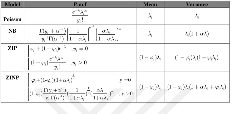
Table 6.1.ZIP, ZINB, Poisson and NB regression models with expectation and variance values

Model P.m.f Mean Varıance

Poisson l_l -! i yi i i e y li li NB a a al a al al -æ ö æ ö G + _{ç ÷÷ ç ÷} ç ÷ ç ÷_÷ ç ÷ ç ç è ø G è + ø + 1 1 1 ( ) 1 ! ( ) 1 1 i y i i i i i y y li li(1+al) ZIP l l j j l j -ì + - = ïï ïï íï - > ïï ïî (1 ) , 0 (1 ) , 0 ! i i i i i i y i i i i e y e y y j l -(1 _i) _i (1-j l_i) (1_i -j l_{i i}) ZINP a a j j al a al j a al al ìïï ïïï í _G ïï ïï G ïî i 1 i i i i 1 -1 y i i -1 i i i i +(1- )(1+ ) ,y =0 (y + ) 1 (1- ) ( ) ( ) , y >0 y ! ( ) 1+ 1+ j l -(1 i) i (1-j li) (1i +ali +j li i)

6.3. Evaluation of the Goodness-of-Fit of the Generalized Linear Models

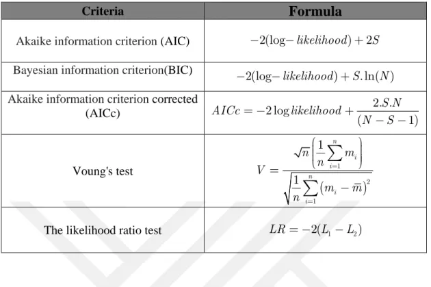
Information critera (IC) are used as the method of choosing the best GLM such as Akaike information criteria (AIC) and Bayesian information criteria (BIC) (Hilbe, 2011).

The two criteria require the sum of two main parts, the natural logarithm of a maximum likelihood and the number of parameters of the model as follows(Hilbe, 2011) ; = -2(log ) 2+ AIC likelihood S (6.26) = -2(log )+ .log( ) BIC likelihood S N (6.27) where,

N: The sample size studied.

S: Estimated number of parameters in the model.

The decision to choose the best GLM by using the AIC and BIC depends on getting the lowest value for these two criteria. (Chen et al., 1993) suggested correcting the bias in the AIC as follows;