T.C.
SELÇUK ÜNİVERSİTESİ FEN BİLİMLERİ ENSTİTÜSÜ
SOME CONTRIBUTIONS TO LIFETIME DISTRIBUTION ANALYSIS
Obaida ADELEI
YÜKSEK LİSANS TEZİ
İstatistik Anabilim Dalını
Ekim-2017 KONYA Her Hakkı Saklıdır
ÖZET
YÜKSEK LİSANS TEZİ
YAŞAM-ZAMANI DAĞILIM ANALİZİNE KATKILAR
Obaida ADELEI
Selçuk Üniversitesi Fen Bilimleri Enstitüsü İstatistik Anabilim Dalı
Prof. Dr. Coşkun KUŞ
2017, 74 Sayfa
Jüri
Yar. Doç. Dr. Ahmet PEKGÖR Prof. Dr. Coşkun KUŞ Doç. Dr. İsmail KINACI
Bu tezde, iki yeni dağılım önerilmiştir. Bu dağılımların dağılım fonksiyonu, kuantil fonksiyonu, hazard ve ters hazard fonksiyonları, değişim katsayısı, momentleri, çarpıklık ve basıklık katsayıları gibi özellikleri gösterilmiştir. İstatistiksel sonuç çıkarımı en çok olabilirlik metodu ile tartışılmıştır. Nelder-Mead simpleks direkt arama, Pattern arama ve genetik algoritması gibi bazı nümerik metotlar en çok olabilirlik tahminlerinin yaklaşık değerlerini bulmak için kullanılmıştır. Simülasyon çalışmasında, en çok olabilirlik tahminlerinin performansları ve en çok olabilirlik tahminlerinin asimptotik özelliklerine dayalı güven aralıklarının kapsama olasılıkları incelenmiştir. Metodoloji nümerik örneklerle örneklendirilmiştir.
Anahtar Kelimeler: Yaşam zamanı dağılımı, En çok olabilirlik tahmini, Monte Carlo simülasyonu, Dağılım modelleme
ABSTRACT
MS THESIS
SOME CONTRIBUTIONS TO LIFETIME DISTRIBUTION ANALYSIS
Obaida ADELEI
GRADUATE SCHOOL OF NATURAL AND APPLIED SCIENCE OF SELÇUK UNIVERSITY
DEGREE OF MASTER OF SCIENCE IN STATICTICS
Prof. Dr. Coşkun KUŞ
2017, 74 Pages
Jury
Yar. Doç. Dr. Ahmet PEKGÖR Prof. Dr. Coşkun KUŞ Doç. Dr. İsmail KINACI
In this thesis, two new distributions are introduced. The distributional properties such as distribution function, quantile function, hazard and reverse hazard functions, moments, coefficient of variation skewness and kurtosis are provided. Statistical inference is discussed by maximum likelihood methodology. Simulation study is performed to investigate the performance of the maximum likelihood estimates and coverage probability of confidence intervals based on asymptotic normality property of maximum likelihood estimates. Several numerical methods such as Nelder-Mead simplex algorithm, Pattern search, simulated annealing algorithm and genetic algorithm are used to get approximate value of maximum likelihood estimates and they are compared. A numerical example is also given to illustrate the methodology.
Keywords: Lifetime distribution, Maximum likelihood estimates, Monte Carlo simulation, Distribution modelling.
ÖNSÖZ
Hayatım boyunca beni en iyi şekilde yetiştiren, her şeyin en iyisine layık olan aileme çok teşekkür ederim.
Geniş bilgi birikimi, yol göstericiliği ve tecrübesi ile çalışmam süresince benden desteğini ve yardımını esirgemeyen Sayın Prof. Dr. Coşkun KUŞ’a sonsuz saygılarımı ve teşekkürlerimi sunarım.
Selçuk Üniversitesi Fen Fakültesi İstatistik bölümünde bana destek olan, hayata dair zorlukları görmemi sağlayan tüm hocalarıma, asistanlara ve arkadaşlarıma teşekkür ederim.
Bu makamda, gerçekleştirdiğim araştırmayı kalbimde büyük yer alan, direnen Filistin Milletine ve bana kapısını açan Türkiye Cumhuriyeti Devletine takdim ederim.
Obaida ADELEI KONYA-2017
ريدقتو ركش
جاملا ةجرد ىلع يلوصح نم هيلا ىعسأو اوبصأ تنك امب ّيلع ّنم يذلا لله دمحلا نم ءاصحلإا يف ريتس .ةيكرتلا اينوق ةنيدم يف قوجلس ةعماج ةبسانملا هذهبو هّجوتأ نأ لاإ ينعسي لا ةبيطلا ميظعو ركشلا ليزجب نانتملاا لاول د نيزيزعلا ّي و يتلئاعل نيذلا اوناك لاوط يل ربكلأا دنسلا يتايح و .هذه ةيميلعتلا يتريسم هجوتأ مث ب يذاتسأ ىلإ نافرعلاو ركشلا هل ناك يذلا ،شوك نكشوج روتكدلا روسيفوربلا زيزعلا يفرشمو مظعلأا رثلأاو ربكلأا لضفلا يف ةعباتم و .يملعلا ثحبلا اذه زاجنا نايسن يننكمي لا ماقملا اذهبو ةناكم نادجولاو بلقلا يف مهل نم ةصاخ لضانملا دماصلا ينيطسلفلا يبعش ، ، ةموكح ايكرت ةلود ابعشو اقفرو يئاقدصأو ءازعلأا يتبرغو يبرد ء اعيمج مكيلإ ... .اذه يلمع جاتن مدقأو يدهأ يليدع ةديبع اينوق -2017CONTENTS ÖZET ... 1 ABSTRACT ... 2 ÖNSÖZ ... 3 CONTENTS ... 5 1. INTRODUCTION ... 6
1.1. Brief History of Reliability ... 6
1.2. Some Fundamental Concepts ... 8
1.2.1. Maximum Likelihood Estimation ... 10
1.3. Some Statistical Distributions ... 11
1.4. The log-logistic Weibull-Poisson distribution ... 15
1.5. Review of the Literature ... 17
2. A NEW COMPOUND LIFETIME DISTRIBUTION-I... 21
2.1. Chen-Weibull Distribution ... 21
2.2. Quantile Function of ChW Distribution ... 23
2.3. Some New and Known Sub-Models of ChW Distribution ... 24
2.4. Hazard and Reverse Hazard Functions of ChW Distribution ... 24
2.5. Moments of ChW Distribution... 27
2.6. Maximum Likelihood Estimation of ChW Distribution ... 30
2.7. Monte Carlo Simulation Study ... 31
3. A NEW COMPOUND LIFETIME DISTRIBUTION-II ... 42
3.1. Chen-Weibull Poisson Distribution ... 42
3.2. Some New and Known Sub-Models of ChWP Distribution ... 44
3.3. Hazard and Reverse Hazard Functions of ChWP Distribution ... 44
3.4. Quantile Function of ChWP Distribution ... 47
3.5. Moments of ChWP Distribution ... 48
3.6. Maximum Likelihood Estimation of ChWP Distribution ... 51
3.7. Monte Carlo Simulation Study ... 54
4. REAL EXAMPLE ... 56
5. CONCLUSIONS AND RECOMMENDATIONS... 60
REFERENCES ... 61
APPENDIX ... 65
1. INTRODUCTION
This chapter consists of five sections, in the first section we address reliability history and its development stages. In Section 2, we discuss some general concepts about reliability and probability distributions. In Section 3, we discuss some statistical distributions which are needed and used in the next chapters. In Section 4, we talk about some references which are address topics of interest. Finally, we address the results of Oluyede study [1] for comparing to the obtained results of this thesis.
1.1. Brief History of Reliability
Reliability is a widely used concept and considered as one of the most important human values through history, it has been celebrated for long times to the present. Reliability as a word and concept was evolved over time according to the applications and the need to regulate and develop the products and its performance. For more details and knowledge about evolution stages of reliability concepts, let’s go in a journey through time with reliability.
The modest beginning was in 1816, and the reliability word was coined for the first time by poet Samuel Taylor Coleridge [2]. In statistics, reliability is the overall consistency of a set of measurements, most of time used to describe tests. Reliability is inversely related to random error [3]. In Psychology, reliability refers to the consistency of a measure. A test reliability will be obtained and valuable ”for all tests” if we can obtain the same result repeatedly [4]. An early application of reliability relates to the telegraph. It was a battery powered system with simple transmitters and receivers connected by wire. A failure might occur due to a broken wire or insufficient power. Also, there were many applications of reliability, but not much new in electronic applications. By 1915, radios with a few vacuum tubes began to appear in the public. Automobiles came into more common use by 1920 and may represent mechanical applications of reliability [5]. In the 1920s, product improvement through the use of statistical quality control was promoted by Dr. Walter A. Shewhart at Bell Labs [6]. In another hand, product reliability was the development of statistics in the 20th century. Statistics as a tool for making measurements would become inseparable with the development of reliability concepts.
At this point, designers were still responsible for reliability and repair people took care of the failures. There wasn’t much planned proactive prevention or economic
justification for doing so. Throughout the 1920s and 30s, Taylor worked on ways to make products more consistent and the manufacturing process more efficient. He was the first to separate the engineering from management and control [7]. In 1927 Charles Lindberg took off in the Spirit from Roosevelt Airfield, Garden City, New York, and landed 33 hours, 30 minutes later at Aéroport Le Bourget in Paris. It was the first solo non-stop transatlantic flight of more than continuous 33 hours, 30 minutes of operation without maintenance [8]. In 1930s, Weibull distribution was created by Wallodie Weibull, who was working in Sweden during this period and investigated the fatigue of materials [9].
Around the end of the 1950s and the start of the 1960s, enthusiasm for the United States was focused on intercontinental ballistic rockets and space explore, particularly associated with the Mercury and Gemini programs. In the race with the Russians to be the primary country to put men on the moon, it was essential that the starting of a kept an eye on shuttle be a win. A relationship for designers working with unwavering quality inquiries was soon settled. The principal diary regarding the matter, IEEE Transactions on dependability turned out in 1963, and various reading material regarding the matter were distributed in the 1960s.
In the 1970s intrigue expanded, in the United States and in addition in different parts of the world, in hazard and wellbeing viewpoints associated with the building and operation of atomic power plants. In the United States, a substantial research commission, drove by Professor Norman Rasmussen was set up to break down the issue. The multimillion dollar extends brought about the alleged Rasmussen report, WASH-1400 (NUREG-75/014). Regardless of its shortcomings, this report speaks to the main genuine security examination of so confounded a framework as an atomic power plant.
Comparative work has additionally been completed in Europe and Asia. In the greater part of businesses, a considerable measure of exertion is directly put on the investigation of hazard and unwavering quality issues. The same is valid in Norway, especially inside the seaward oil industry. The seaward oil and gas advancement in the North Sea is by and by advancing into more profound and more threatening waters, and an expanding number of remotely worked subsea generation frameworks are put into operation. The significance of the unwavering quality of subsea frameworks is in many regards parallel to the dependability of shuttles. A low dependability can't be remunerated by broad upkeep [10].
Finally, the reliability, according to ISO 8402, is the ability of an item to perform a required function, under given environmental and operational conditions and for a stated period of time.
1.2. Some Fundamental Concepts
We will use definitions and concepts of interest in this research. The most used of those are given in this section. In this Section, definitions are given for non-negative continuous random variables.
Definition 1.1 The reliability function of lifetime (𝑇) of an item is the probability that the item does not fail in the time interval (0, 𝑡], defined by
𝑅(𝑡) = 1 − 𝐹(𝑡) = 𝑃(𝑇 > 𝑡), 𝑓𝑜𝑟 𝑡 > 0, where 𝐹(. ) is the cumulative distribution function (cdf) of 𝑇. In continuous case, one can write
𝑅(𝑡) = 1 − ∫ 𝑓(𝑢)𝑑𝑢 𝑡 0 = ∫ 𝑓(𝑢)𝑑𝑢 ∞ 𝑡 ,
where 𝑓(. ) is the probability density function (pdf) of 𝑇. 𝑅(𝑡) is also called the survivor function [10].
Definition 1.2 The cumulative distribution function of a random variable (r.v) 𝑋, denoted by 𝐹𝑋(𝑥), is defined by [10]
𝐹𝑋(𝑥) = 𝑃(𝑋 ≤ 𝑥), 𝑥 ∈ ℝ.
Definition 1.3 The probability density function of a continuous random variable 𝑋, denoted by 𝑓𝑋(𝑥), is the function that satisfies
𝐹𝑋(𝑥) = ∫ 𝑓𝑋(𝑡)𝑑𝑡 𝑥
0
, where 𝑓𝑋(𝑥) > 0, 𝑓𝑜𝑟 𝑎𝑙𝑙 𝑥, [10].
Definition 1.4 The failure rate or hazard function is defined by ℎ(𝑡) = 𝑙𝑖𝑚 ∆𝑡→0 𝑃𝑟 (𝑡 ≤ 𝑇 < 𝑡 + ∆𝑡|𝑇 ≥ 𝑡) ∆𝑡 , =𝑓(𝑡) 𝑅(𝑡) = −𝑅 ′(𝑡) 𝑅(𝑡).
The hazard function specifies the instantaneous rate of death [11].
Definition 1.5 The reverse hazard function or reverse hazard rate is defined as
ℎ(𝑡) = 𝑓(𝑡)
𝐹(𝑡), 𝑓𝑜𝑟 𝑡 > 0.
Theorem 1.1 Let us consider continuous random variables 𝑋𝑖’s (𝑖 = 1, … , 𝑚) with
survival function 𝑅𝑖 and hazard function ℎ𝑖. Furthermore, 𝑋𝑖’s are to be independent. Then the compound random variable 𝑋 = min(𝑋1, 𝑋2, … , 𝑋𝑚) has pdf, cdf and hazard functions of the forms
𝑓𝑐𝑜𝑚𝑝(𝑥) = (∏ 𝑅𝑗 𝑚 𝑗=1 (𝑥)) (∑ ℎ𝑗(𝑥) 𝑚 𝑗=1 ), (1.1) 𝐹𝑐𝑜𝑚𝑝(𝑥) = 1 − (∏ 𝑅𝑗 𝑚 𝑗=1 (𝑥)), (1.2) and ℎ𝑐𝑜𝑚𝑝(𝑥; 𝝍) = (∑ ℎ𝑗(𝑥) 𝑚 𝑗=1 ), (1.3) respectively. Proof: 𝐹𝑐𝑜𝑚𝑝(𝑥) = 𝑃(𝑋 ≤ 𝑥) = 1 − 𝑃(𝑋 > 𝑥)
= 1 − 𝑃(min(𝑋1, 𝑋2, … , 𝑋𝑚) > 𝑥) = 1 − 𝑃(𝑋1 > 𝑥, 𝑋2 > 𝑥, … , 𝑋𝑚 > 𝑥) = 1 − 𝑃(𝑋1 > 𝑥)𝑃(𝑋2 > 𝑥) … 𝑃(𝑋𝑚 > 𝑥) = 1 − 𝑅1(𝑥)𝑅2(𝑥) × ⋯ × 𝑅𝑚(𝑥). = 1 − ∏ 𝑅𝑗 𝑚 𝑗=1 (𝑥).
Eq. (1.4) and Eq. (1.6) follows from Eq. (1.5). Note that these results are well-known but there is no any source to cite them.
Theorem 1.2 Let the random variable 𝑋 with pdf 𝑓, then an approximated 𝑟th moment of 𝑋 is given by 𝜇𝑟′ = ∑ 𝜔̅𝑖 2 (1 − 𝑦𝑖)2 𝑁 𝑖=1 (1 + 𝑦𝑖 1 − 𝑦𝑖) 𝑟 𝑓 (1 + 𝑦𝑖 1 − 𝑦𝑖) , 𝑟 = 1,2, … (1.4) where 𝑦𝑖’s are the zeros and the corresponding Christoffel numbers of the
Legendre-Gauss quadrature formula on the interval (-1, 1), where
𝜔̅𝑖 = 2
(1 − 𝑦𝑖2)(𝐿′𝑁+1(𝑦𝑖))
2 , 𝐿′𝑁+1(𝑦𝑖) =
𝑑𝐿𝑁+1(𝑦)
𝑑𝑦 𝑎𝑡 𝑦 = 𝑦𝑖,
and 𝐿𝑁(∙) is the Legendre polynomial of degree 𝑁 [9].
1.2.1. Maximum Likelihood Estimation
The method of maximum likelihood is the most commonly used procedure for deriving estimators. Solution of the likelihood equations give us the extreme values of the likelihood function. These extreme values are called the maximum likelihood estimates (MLEs). Recall that if 𝑋1, … , 𝑋𝑛 are iid sample from a population with pdf 𝑓(𝑥|𝜽), the likelihood function is defined by
𝐿(𝜽|𝒙) = 𝐿(𝜽|𝒙) = ∏ 𝑓(𝑥𝑖|𝜽)
𝑛
𝑖=1
where 𝜽 = (𝜃1, … , 𝜃𝑘) and 𝒙 = (𝑥1, … , 𝑥𝑛). For each sample point 𝒙, let 𝜽̂(𝒙) be a parameter value at which 𝐿(𝜽|𝒙) attains its maximum as a function in 𝜽, with 𝒙 held fixed. A MLE of the parameter 𝜽 based on a sample 𝑿 is 𝜃̂(𝑿) = arg max 𝐿(𝜽|𝒙). The natural logarithm of 𝐿(𝜽|𝒙) is as follows:
log 𝐿(𝜽|𝒙) = ∑ log 𝑓(𝒙|𝜽)
𝑛
𝑖=1
(1.2.2)
If the likelihood function is differentiable in 𝜃𝑖, then it is said to be the candidates for the MLE are the values of (𝜃1, … , 𝜃𝑘) that solve [12]
𝜕
𝜕𝜃𝑖log 𝐿(𝜽|𝒙) = 0, 𝑖 = 1, … , 𝑘. (1.2.3)
1.3. Some Statistical Distributions
In this section, we discussed some probability distributions that will be used in the next sections. These lifetime distributions are given below:
• The exponential Distribution
The pdf and the cdf of the exponential distribution are given, respectively, by
𝑓𝐸(𝑥; 𝛼) = 𝛼𝑒−𝛼𝑥, 𝑥 > 0 (1.3.1)
and
𝐹𝐸(𝑥; 𝛼) = 1 − 𝑒−𝛼𝑥, 𝑥 > 0, (1.3.2)
where 𝛼 > 0 is scale parameter [11]. • Weibull Distribution
Weibull distribution is one of the most commonly used model in reliability applications and lifetime data analysis. The pdf and the cdf of the Weibull distribution are given, respectively, by
𝑓𝑊(𝑥; 𝛼, 𝛽) = 𝛼𝛽𝑥𝛽−1𝑒−𝛼𝑥
𝛽
, 𝑥 > 0 (1.3.3) and
𝐹𝑊(𝑥; 𝛼, 𝛽) = 1 − 𝑒−𝛼𝑥
𝛽
, 𝑥 > 0, (1.3.4) where 𝛼 > 0 is a scale parameter and 𝛽 > 0 is known as the shape parameter [13]. It can be noticeable that the exponential distribution is a special case of a Weibull distribution, when 𝛽 = 1, the Weibull distribution is reduced to the exponential distribution. Hazard and reliability functions of the Weibull distribution are given, respectively, by
ℎ𝑊(𝑥; 𝛼, 𝛽) = 𝛼𝛽𝑥𝛽−1, (1.3.5) and 𝑅𝑊(𝑥; 𝛼, 𝛽) = 𝑒−𝛼𝑥 𝛽 . (1.3.6) • Burr-XII Distribution
Burr XII distribution is most commonly used to model household income. The pdf and the cdf of Burr type XII distribution are given, respectively, by
𝑓𝐵(𝑥; 𝑠, 𝑐, 𝑘) =𝑐𝑘 𝑠 ( 𝑥 𝑠) 𝑐−1 (1 + (𝑥 𝑠) 𝑐 ) −(𝑘+1) , 𝑥 > 0, (1.3.7) and 𝐹𝐵(𝑥; 𝑠, 𝑐, 𝑘) = 1 − (1 + ( 𝑥 𝑠) 𝑐 ) −𝑘 , 𝑥 > 0, (1.3.8) where the parameters 𝑠 > 0 is scale parameter and 𝑐, 𝑘 > 0 are both the shape parameters of the distribution [14]. The Hazard and reliability functions of Burr-XII distribution are given, respectively, by ℎ𝐵(𝑥; 𝑠, 𝑐, 𝑘) = (1 + (𝑥 𝑠) 𝑐 ) −𝑘𝑐 𝑠( 𝑥 𝑠) 𝑐−𝑘 , 𝑥 > 0 (1.3.9) and 𝑅𝐵(𝑥; 𝑠, 𝑐, 𝑘) = (1 + ( 𝑥 𝑠) 𝑐 ) −𝑘 , 𝑥 > 0. (1.3.10)
• Log-logistic Distribution
The log-logistic distribution (LLoG) is known as the Fisk distribution in economics. The pdf and cdf the following forms
𝑓𝐿𝐿𝑜𝐺(𝑥; 𝑠, 𝑐) = (𝑐 𝑠⁄ )(𝑥 𝑠⁄ )𝑐−1 [1 + (𝑥/𝑠)𝑐]2 , 𝑥 > 0, (1.3.11) and 𝐹𝐿𝐿𝑜𝐺(𝑥; 𝑠, 𝑐) = 1 1 + (𝑥 𝑠⁄ )−𝑐, 𝑥 > 0, (1.3.12)
respectively, where 𝑠 > 0 is scale parameter and 𝑐 > 0 is the shape parameter. The log-logistic obtains its name from the fact that 𝑌 = log(𝑇) has a log-logistic distribution with pdf
𝑓(𝑦) = 𝜎
−1exp[(𝑦 − 𝜇)/𝜎]
(1 + exp[(𝑦 − 𝜇)/𝜎])2, − ∞ < 𝑦 < ∞
where 𝜇 = log 𝑠 and 𝜎 = 𝑐−1, therefore −∞ < 𝜇 < ∞ and 𝜎 > 0 [11]. Here, it can be also noticeable that the log-logistic distribution is a special case of Burr-XII distribution, when 𝑘 = 1, Burr-XII distribution is reduced to the log-logistic distribution. The hazard and reliability functions of log-logistic distribution are given, respectively, by
ℎ𝐿𝐿𝑜𝐺(𝑥; 𝑠, 𝑐) = (1 + (𝑥 𝑠) 𝑐 ) −1𝑐 𝑠( 𝑥 𝑠) 𝑐−1 (1.3.13) and 𝑅𝐿𝐿𝑜𝐺(𝑥; 𝑠, 𝑐) = (1 + (𝑥 𝑠) 𝑐 ) −1 . (1.3.14) • Poisson Distribution
Poisson distribution is often used in estimating the number of occurrence over specified interval of time or space, etc. For example, it is used for predicting the number of phone calls arriving at a given telephone exchange within a certain period of time. A discrete random variable 𝑋 is said to have a Poisson distribution if its probability mass function (pmf) is given by
𝑓(𝑘; 𝜃) =𝑒
−𝜃𝜃𝑘
𝑘! , 𝑘 = 0,1,2, … , 𝜃 > 0 (1.3.15)
where 𝜃 is the average number of occurrence of an event per unit of measurement, and 𝑘 is the number of occurrence of an event per unit of measurement [15]. For seeing applications about the Poisson distribution, the reader should see [16].
• The zero truncated Poisson Distribution
The zero-truncated Poisson (ZTP) distribution is a certain discrete probability distribution whose support is the set of positive integers. This distribution is also known as the conditional Poisson distribution or the positive Poisson distribution. It is the conditional probability distribution of Poisson-distributed random variable, given that the value of the random variable is not zero [15]. The pmf 𝑔(𝑘; 𝜃) of the ZTP is given by
𝑔(𝑘; 𝜃) = 𝑃(𝑋 = 𝑘|𝑋 > 0) = 𝑓(𝑘, 𝜃) 1 − 𝑓(0, 𝜃) =
𝜃𝑘𝑒−𝜃
𝑘! (1 − 𝑒−𝜃). (1.3.16)
where 𝑓 is pmf of Poisson distribution with mean 𝜃. • Chen Distribution
Let 𝑋 be the random variable from Chen distribution, then the pdf and cdf of 𝑋 are given, respectively, by 𝑓𝐶ℎ(𝑥; 𝜆, 𝛿) = 𝜆𝛿𝑥𝛿−1𝑒𝜆(1−𝑒𝑥𝛿)+𝑥𝛿 , 𝑥 > 0 (1.3.17) and 𝐹𝐶ℎ(𝑥; , 𝜆, 𝛿) = 1 − 𝑒𝜆(1−𝑒 𝑥𝛿) , 𝑥 > 0 (1.3.18)
where 𝜆 > 0 and 𝛿 > 0 are the distribution parameters [17]. Hazard and reliability functions of Chen distribution are given by
ℎ𝐶ℎ(𝑥; 𝜆, 𝛿) = 𝜆𝛿𝑥𝛿−1𝑒𝑥 𝛿 , (1.3.19) and 𝑅𝐶ℎ(𝑥; , 𝜆, 𝛿) = 𝑒𝜆(1−𝑒𝑥𝛿), 𝑥 > 0, (1.3.20) respectively.
• Gompertz Distribution
Gompertz distribution is often applied to describe the distribution of adult lifespans by demographers and actuaries. The pdf and the cdf of Gompertz distribution are given, respectively, by
𝑓𝐺𝑧(𝑥; 𝜆, 𝛽) = 𝜆𝛽𝑒𝜆(1−𝑒𝛽𝑥)+𝛽𝑥, 𝑥 > 0 (1.3.21)
and
𝐹𝐺𝑧(𝑥; 𝜆, 𝛽) = 1 − 𝑒𝜆(1−𝑒𝛽𝑥), 𝑥 > 0, (1.3.22)
where 𝛽 > 0 is the scale parameter and 𝜆 > 0 is the shape parameter of Gompertz distribution [18].
• Rayleigh Distribution
Rayleigh distribution is a special case of Weibull distribution when 𝛽 = 2, regularly. The pdf and the cdf of Rayleigh distribution are, respectively, of the forms
𝑓𝑅(𝑥; 𝛼) = 2𝛼𝑥𝑒−𝛼𝑥2, 𝑥 > 0 (1.3.23)
and
𝐹𝑅(𝑥; 𝛼) = 1 − 𝑒−𝛼𝑥
2
, 𝑥 > 0, (1.3.24) where 𝛼 > 0 is the scale parameter of the distribution [19].
1.4. The log-logistic Weibull-Poisson distribution
In this section, we discuss the results of Oluyede et al. [1] and [20]. Since our study based on their method, we give some details of their results. In general, they presented a generalized extended Weibull (GEW) distribution with cdf of the following form
𝐺(𝑥; 𝚯, 𝛙) = 1 − 𝐵(𝑥; 𝛙) exp(−𝛼𝐻(𝑥; 𝚯)), (1.4.1) where 𝐵(𝑥; 𝛙) > 0 is a continuous function, 𝐻(𝑥; 𝚯) is a non-negative monotonically increasing function that is depends on the vectors of parameters 𝛙 and 𝚯, respectively. For obtaining the Log-Logistic Weibull (LLoGW) distribution, they gave 𝐵(𝑥; 𝛙) =
(1 + (𝑥 𝑠⁄ )𝑐)−1 and 𝐻(𝑥; 𝚯) = 𝑥𝛽. The cdf and pdf of the LLoGW distribution are given, respectively, by 𝐹𝐿𝐿𝑜𝐺𝑊(𝑥; 𝑠, 𝑐, 𝛼, 𝛽) = 1 − (1 + (𝑥 𝑠) 𝑐 ) −1 𝑒−𝛼𝑥𝛽, (1.4.2) and 𝑓𝐿𝐿𝑜𝐺𝑊(𝑥) = (1 + (𝑥 𝑠) 𝑐 ) −1 𝑒−𝛼𝑥𝛽(𝛼𝛽𝑥𝛽−1+ (1 + (𝑥 𝑠) 𝑐 ) −1𝑐 𝑠( 𝑥 𝑠) 𝑐−1 ), (1.4.3)
where 𝑥 > 0 and 𝑠, 𝑐, 𝛼, 𝛽 > 0 [20]. The hazard rate and reliability functions of the LLoGW distribution are given, respectively, by [20]
ℎ𝐿𝐿𝑜𝐺𝑊(𝑥) = (1 + (𝑥 𝑠) 𝑐 ) −1𝑐 𝑠( 𝑥 𝑠) 𝑐−1 + 𝛼𝛽𝑥𝛽−1 (1.4.4) and 𝑅𝐿𝐿𝑜𝐺𝑊(𝑥; 𝑠, 𝑐, 𝛼, 𝛽) = (1 + (𝑥 𝑠) 𝑐 ) −1 𝑒−𝛼𝑥𝛽, (1.4.5)
The log-logistic Weibull-Poisson (LLoGWP) distribution has been introduced by assuming the random variable 𝑋~𝐿𝐿𝑜𝐺𝑊 with cdf and pdf given in Eq. (1.4.2) and Eq. (1.4.3), respectively. Given 𝑁, let 𝑋1, . . . , 𝑋𝑁 be independent and identically distributed random variables from the LLoGW distribution. Let 𝑁 be distributed according to the zero truncated Poisson distribution with pdf (1.3.16). The cdf and pdf of the LLoGW distribution of 𝑋|𝑁 = 𝑛 where 𝑋 = 𝑚𝑎𝑥(𝑋1, . . . , 𝑋𝑁) are given, respectively, by
𝐺𝑋|𝑁=𝑛(𝑥; 𝑠, 𝑐, 𝛼, 𝛽, 𝑛) = [𝐹𝐿𝐿𝑜𝐺𝑊(𝑥)]𝑛
(1.4.7)
and
𝑔𝑋|𝑁=𝑛(𝑥) = 𝑛[𝐹𝐿𝐿𝑜𝐺𝑊(𝑥)]𝑛−1 𝑓𝐿𝐿𝑜𝐺𝑊(𝑥), (1.4.8)
where 𝑠, 𝑐, 𝛼, 𝛽 > 0, 𝑥 > 0 [1]. 𝐹𝐿𝐿𝑜𝐺𝑊(𝑥), 𝑓𝐿𝐿𝑜𝐺𝑊(𝑥) also, are given in Eq. (1.4.2) and Eq. (1.4.3) respectively. Eq. (1.4.7) and Eq. (1.4.8) can be, respectively, rewritten as
𝐹𝐸𝐿𝐿𝑜𝐺𝑊(𝑥; 𝑠, 𝑐, 𝛼, 𝛽, 𝑛) = [𝐹𝐿𝐿𝑜𝐺𝑊(𝑥)]𝑛 (1.4.9)
and
for 𝑠, 𝑐, 𝛼, 𝛽 > 0 and 𝑥 > 0 [1]. From the previous, it can be said that the exponentiated log-logistic Weibull (ELLoGW) distribution has been obtained. The marginal cdf of 𝑋 defines the LLoGWP distribution as follows:
Now, by using the Eq. (1.4.11), the marginal cdf is given by
𝐹𝐿𝐿𝑜𝐺𝑊𝑃(𝑥; 𝑠, 𝑐, 𝛼, 𝛽, 𝜃) = ∑[𝐺𝑋|𝑁=𝑛(𝑥) ∞ 𝑛=1 𝑃(𝑁 = 𝑛)], = 1 − 𝑒 𝜃𝐹𝐿𝐿𝑜𝐺𝑊(𝑥) 1 − 𝑒𝜃 , (1.4.12) where 𝑠, 𝑐, 𝛼, 𝛽, 𝜃 > 0, 𝑥 > 0 and 𝐹𝐿𝐿𝑜𝐺𝑊(𝑥) = 1 − (1 + (𝑥 𝑠⁄ )𝑐)−1𝑒−𝛼𝑥 𝛽 was given in Eq. (1.4.2) [1]. This distribution is called LLoGWP [1]. The pdf of the LLoGWP distribution is also given by
𝑓𝐿𝐿𝑜𝐺𝑊𝑃(𝑥; 𝑠, 𝑐, 𝛼, 𝛽, 𝜃) =
𝜃𝑓𝐿𝐿𝑜𝐺𝑊(𝑥)𝑒𝜃𝐹𝐿𝐿𝑜𝐺𝑊(𝑥)
𝑒𝜃− 1 , (1.4.13)
where 𝑠, 𝑐, 𝛼, 𝛽, 𝜃 > 0 and 𝑥 > 0 ) [1]. 1.5. Review of the Literature
Lee, Famoye and Olumolade (2007) discussed some properties of a four-parameter beta-Weibull distribution. The beta-beta-Weibull distribution can have bathtub, unimodal, increasing, and decreasing hazard functions. It is applied to censored data sets on bus-motor failures and a censored data set on head-and neck- cancer clinical trial. A simulation is performed to compare the beta-Weibull distribution with the exponentiated Weibull distribution [21].
Percontini, Blas and Cordeiro (2013) studied a new and wider distribution of five-parameter, it is called the beta Weibull Poisson, which is obtained by compounding the Weibull Poisson and beta distributions. It generalizes several known lifetime models [22].
Kus (2007) introduced a new lifetime distribution of two-parameter with decreasing failure rate and discussed different properties of the introduced distribution. The EM algorithm is used to get the maximum likelihood estimates and the asymptotic variances
and covariance are studied. Simulation studies are performed in order to assess the accuracy of the approximation of the variances and covariance of the maximum likelihood estimates and investigate the convergence of the proposed EM scheme [23].
Lu and Shi (2012) introduced a new compounding distribution, called the Weibull– Poisson distribution. The shape of failure rate function of the new compounding distribution is flexible, it can be decreasing, increasing, upside-down bathtub-shaped or unimodal. A comprehensive mathematical treatment of the proposed distribution and expressions of its density, cumulative distribution function, survival function, failure rate function, the kth raw moment and quantiles are provided. They discussed asymptotic properties of the maximum likelihood estimates, and intensive simulation studies are conducted for evaluating the performance of parameter estimation [24].
Mahmoudi and Sepahdar (2013) proposed a new four-parameters distribution with increasing, decreasing, bathtub-shaped and unimodal failure rate, called as the exponentiated Weibull–Poisson (EWP) distribution. The new distribution arises on a latent complementary risk problem base and is obtained by compounding exponentiated Weibull (EW) and Poisson distributions. They obtained several properties of the new distribution such as its probability density function, its reliability and failure rate functions, quantiles and moments. The maximum likelihood estimation procedure via an EM-algorithm is presented in their paper. Sub-Models of the EWP distribution are studied in details [25].
Barreto-Souza and Cribari-Neto (2009) generalized the EP distribution, which was introduced by Kuş (2007), and show that the failure rate of the new distribution can be decreasing or increasing. The failure rate can also be upside-down bathtub shaped. A comprehensive mathematical treatment of the new distribution is provided. They provided closed-form expressions for the density, cumulative distribution, survival and failure rate functions; and also obtained the density of the 𝑖𝑡ℎ order statistic. They derived
the 𝑟th raw moment of the new distribution and also the moments of order statistics. Moreover, they discussed estimation by maximum likelihood and obtained an expression for Fisher's information matrix [26].
Cancho, Louzada-Neto and Barriga (2011) in their paper, proposed a new two-parameters lifetime distribution with increasing failure rate. The new distribution arises
on a latent complementary risk problem base. The properties are discussed, including a formal proof of its probability density function and explicit algebraic formulae for its reliability and failure rate functions, quantiles and moments, including the mean and variance [27].
Oluyede, Foya, Warahena-Liyanage and Huang (2015) developed and addressed a new generalized distribution called the log-logistic Weibull (LLoGW). The structural properties of the distribution including the hazard function, reverse hazard function, quantile function, probability weighted moments, moments, conditional moments, mean deviations, Bonferroni and Lorenz curves, distribution of order statistics, L moments and Renyi entropy are derived. Method of maximum likelihood is used to estimate the parameters of this new distribution [28].
Paranaiba, Ortega, Cordeiro and Pescim (2011) defined and investigated for the first time, beta Burr XII distribution of a five-parameter. The new distribution contains as special Sub-Models some well-known distributions discussed in the literature, such as the logistic, Weibull and Burr XII distributions, among several others. Its moment generating function was derived. A special case, the moment generating function of the Burr XII distribution was obtained, which seems to be a new result. Moments, mean deviations, Bonferroni and Lorenz curves and reliability were provided. They derived two representations for the moments of the order statistics. The method of maximum likelihood and a Bayesian analysis were proposed for estimating the model parameters. For different parameter settings and sample sizes, various simulation studies were performed and compared in order to study the performance of the new distribution [29]. Santos-Silva and Tenreyro (2010) noted that the existence of the maximum likelihood estimates in Poisson regression depends on the data configuration, and proposed a strategy to identify the existence of the problem and to single out the regressors causing it [30].
Xia, Mi and Zhou (2009) shown the existence and uniqueness of the maximum likelihood estimators of the two parameters of the underlying lognormal distribution with Type-I censored data and grouped data. They established the proof under the case of normal distribution and extended to the lognormal distribution through invariance
property, and applied the result to estimate the median and mean of the lognormal population [31].
Huang and Oluyede (2014) proposed and studied a new family of distributions called exponentiated Kumaraswamy-Dagum (EKD) distribution, which includes several well-known sub-models. Statistical properties including series representation of the probability density function, hazard and reverse hazard functions, moments, mean and median deviations, reliability, Bonferroni and Lorenz curves, as well as entropy measures for this class of distributions and the sub-models were presented. Maximum likelihood estimates of the model parameters were obtained [32].
Bidram, Behboodian and Towhidi (2013) proposed a new distribution called beta Weibull-geometric (BWG) distribution, which is generated from the logit of a beta random variable and includes the Weibull geometric distribution [33].
Cooray and Ananda (2008) presented a two-parameter family of lifetime distribution which is derived from a model for static fatigue. The cumulative distribution function (cdf) of this new family is quite similar to the cdf of the half-normal distribution, and therefore this density is referred to as the generalized half-normal distribution (GHN). Even though the GHN distribution is a two-parameter distribution, the hazard rate function can form variety of shapes such as monotonically increasing, monotonically decreasing, and bathtub shapes. Some properties of this family were given, and examples were cited to compare with other commonly used failure time distributions such as Weibull, gamma, lognormal, and Birnbaum-Saunders [34].
2. A NEW COMPOUND LIFETIME DISTRIBUTION-I
In this chapter, we introduce a new lifetime distribution by compounding Chen and Weibull distributions. The compounding method used in [20], which is discussed in the study. Some distributional properties such as moments, quantiles, hazard function and etc. are investigated. Maximum likelihood method is used to estimate the distribution parameters.
2.1. Chen-Weibull Distribution
In this section, we introduce a new lifetime distribution, compounding Chen and Weibull distributions, by using the general formula of the developed generalized extended Weibull (GEW) distribution [1]. The cdf of GEW is given by Eq. (1.4.1) as follows
𝐺(𝑥; 𝚯, 𝛙) = 1 − 𝐵(𝑥; 𝛙) exp(−𝛼𝐻(𝑥; 𝚯)), (2.1.1) where 𝐵(𝑥; 𝛙) > 0 is a continuous function, 𝐻(𝑥; 𝚯) is a non-negative monotonically increasing function that is depends on the vectors of parameters 𝛙 and 𝚯, respectively. In this chapter we choose
𝐵(𝑥; 𝛙) = 𝑒𝜆(1−𝑒𝑥𝛿), (2.1.2)
and
𝐻(𝑥; 𝚯) = 𝑥𝛽. (2.1.3)
By using (2.1.2) and (2.1.3) in Eq. (2.1.1), then the cdf of ChW distribution is given by
𝐹𝐶ℎ𝑊(𝑥; 𝜆, 𝛿, 𝛼, 𝛽) = 1 − 𝑒𝜆(1−𝑒𝑥𝛿)𝑒−𝛼𝑥𝛽, (2.1.4)
for 𝑥 > 0 and 𝜆, 𝛿, 𝛼, 𝛽 > 0. According to Theorem 1.1, the pdf of ChW distribution is also given by
𝑓𝐶ℎ𝑊(𝑥; 𝜆, 𝛿, 𝛼, 𝛽) = (ℎ𝐶ℎ+ ℎ𝑊)𝑅𝐶ℎ𝑊,
= (𝜆𝛿𝑥𝛿−1𝑒𝑥𝛿+ 𝛼𝛽𝑥𝛽−1) 𝑒𝜆(1−𝑒𝑥𝛿)𝑒−𝛼𝑥𝛽, (2.1.5)
for 𝑥 > 0 and 𝜆, 𝛿, 𝛼, 𝛽 > 0. Hazard and reliability functions of ChW distribution are given, respectively, by
ℎ𝐶ℎ𝑊(𝑥; 𝜆, 𝛿, 𝛼, 𝛽) = ℎ𝐶ℎ+ ℎ𝑊
= 𝜆𝛿𝑥𝛿−1𝑒𝑥𝛿+ 𝛼𝛽𝑥𝛽−1, (2.1.6)
and
𝑅𝐶ℎ𝑊(𝑥; 𝜆, 𝛿, 𝛼, 𝛽) = 𝑅𝐶ℎ𝑅𝑊
= 𝑒𝜆(1−𝑒𝑥𝛿)𝑒−𝛼𝑥𝛽. (2.1.7) In the next Fig. 2.1 and Fig. 2.2, we plot pdf’s for ChW distribution at different values of 𝜆, 𝛿, 𝛼 and 𝛽. A Matlab code is given in Appendix.
Figure 2.2. pdf plots of ChW distribution for various values of 𝜆, 𝛿, 𝛼 and 𝛽.
2.2. Quantile Function of ChW Distribution
The quantile function is defined by 𝑥𝑝 = 𝐹−1(𝑝) for 𝑝 ∈ (0,1). The quantile function of
ChW distribution is obtained by solving the following equation
𝛼𝑥𝛽− 𝜆 (1 − 𝑒𝑥𝛿) + log(1 − 𝑝) = 0. (2.2.1)
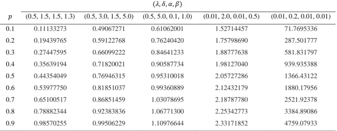
Numerically, we can generate the random numbers of the quantiles based on the above equation. For computing the quantiles of ChW distributions, a Matlab code is given in Appendix. In the Table 2.1, we have been computed quantiles for various values of 𝜆, 𝛿, 𝛼 and 𝛽.
Table 2.1. ChW quantiles for some selected values (𝜆, 𝛿, 𝛼, 𝛽) 𝑝 (0.5, 1.5, 1.5, 1.3) (0.5, 3.0, 1.5, 5.0) (0.5, 5.0, 0.1, 1.0) (0.01, 2.0, 0.01, 0.5) (0.01, 0.2, 0.01, 0.01) 0.1 0.11133273 0.49067271 0.61062001 1.52714457 71.7695336 0.2 0.19439765 0.59122768 0.76240420 1.75798690 287.501777 0.3 0.27447595 0.66099222 0.84641233 1.88777638 581.831797 0.4 0.35639194 0.71820021 0.90587734 1.98127040 939.935388 0.5 0.44354049 0.76946315 0.95310018 2.05727286 1366.43122 0.6 0.53977750 0.81851037 0.99360889 2.12432179 1880.17956 0.7 0.65100517 0.86851459 1.03078695 2.18787780 2521.92378 0.8 0.78882344 0.92383836 1.06771300 2.25342773 3384.89086 0.9 0.98570255 0.99506229 1.10976644 2.33171852 4759.07933
2.3. Some New and Known Sub-Models of ChW Distribution
We can obtain several distributions from the supposed ChW distribution as follows: • If 𝛿 = 𝛽 = 1, we obtain Gompertz-exponential (GzE) distribution.
• If 𝛿 = 1 and 𝛽 = 2, we obtain Gompertz-Rayleigh (GzR) distribution [35]. • If 𝛿 = 1 and 𝛼 → 0, we have Gompertz (Gz) distribution. See Eq. (1.3.22).
• If 𝜆 → 0, we obtain Weibull distribution. See Eq. (1.3.4).
• If 𝜆 → 0 and 𝛽 = 1, we obtain the exponential (E) distribution. See Eq. (1.3.2). • If 𝛽 = 1, we have Chen exponential distribution [4].
• If 𝛽 = 2, we have Chen Rayleigh (ChR) distribution.
• If 𝜆 → 0 and 𝛽 = 2, we obtain Rayleigh (R) distribution. See Eq. (1.3.24).
2.4. Hazard and Reverse Hazard Functions of ChW Distribution
In this section, hazard and reverse hazard functions for ChW distribution will be presented. We will give a different and selected values of 𝜆, 𝛿, 𝛼 and 𝛽 for the hazard and reverse hazard plots. By using the Eq. (1.3.5) and Eq. (1.3.17), according to Theorem 1.1, hazard and reverse hazard functions of ChW distribution are given, respectively, by
ℎ𝐶ℎ𝑊(𝑥; 𝜆, 𝛿, 𝛼, 𝛽) = ℎ𝐶ℎ+ ℎ𝑊, = 𝜆𝛿𝑥𝛿−1𝑒𝑥𝛿+ 𝛼𝛽𝑥𝛽−1, (2.4.1) and 𝜏𝐶ℎ𝑊(𝑥) = 𝑅𝐶ℎ𝑊(ℎ𝐶ℎ+ ℎ𝑊) 1 − 𝑅𝐶ℎ𝑊 , = 𝑒 𝜆(1−𝑒𝑥𝛿) 𝑒−𝛼𝑥𝛽(𝜆𝛿𝑥𝛿−1𝑒𝑥𝛿+ 𝛼𝛽𝑥𝛽−1) 1 − 𝑒𝜆(1−𝑒𝑥𝛿) 𝑒−𝛼𝑥𝛽 , (2.4.2) for 𝑥 > 0 and 𝜆, 𝛿, 𝛼, 𝛽 > 0.
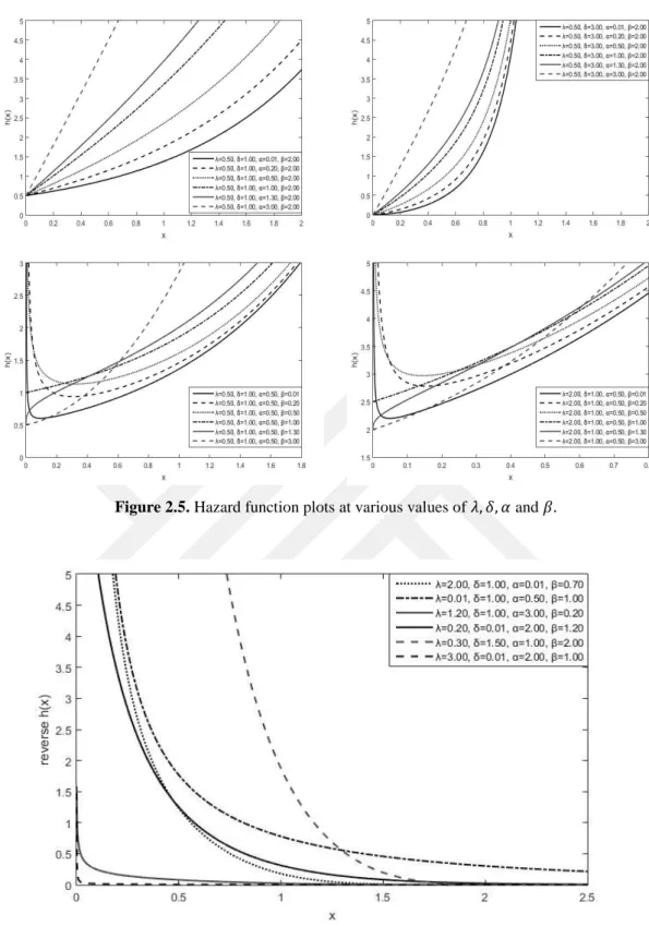
The graphs of hazard and reverse hazard functions for different values of the parameters 𝜆, 𝛿, 𝛼 and 𝛽 have been given in the Fig. 2.3, Fig. 2.4, Fig. 2.5 and Fig. 2.6, respectively.
Figure 2.3. Hazard function plots at various values of 𝜆, 𝛿, 𝛼 and 𝛽.
Figure 2.5. Hazard function plots at various values of 𝜆, 𝛿, 𝛼 and 𝛽.
Figure 2.6. Reverse hazard function plots at various values of 𝜆, 𝛿, 𝛼 and 𝛽.
The plots of the hazard function for various values of the parameters 𝜆, 𝛿, 𝛼 and 𝛽 are given in Fig. 2.3, Fig. 2.4 and Fig.2.5. These plots show us different shapes such as monotonically increasing, monotonically decreasing and bathtub shapes. This feature indicates to the importance of ChW distribution, which show us the suitability for monotonic and non-monotonic hazard behaviours under real life conditions.
2.5. Moments of ChW Distribution
Numerically, the moments and related measures of ChW distribution, such as standard deviation (SD), coefficient of variation (CV), coefficient of skewness (CS) and coefficient of kurtosis (CK) can be obtained by using Theorem 1.2. In general,the 𝑟-the moment of r.v 𝑋 which is distributed ChW is given by
𝜇𝑟′ = 𝐸(𝑋𝑟) = ∫ 𝑥𝑟𝑓 𝐶ℎ𝑊𝑑𝑥 ∞
0
, (2.5.1)
where 𝑓𝐶ℎ𝑊 is defined in Eq. (2.1.5). Theorem 1.2 has been used to obtain approximated SD, CV, CS, CK and the first six moments. Matlab codes to obtain these measures are given in the Appendix. The SD, CV, CS and CK are, respectively, given by
𝑆𝐷 = 𝜎 = √𝐸(𝑋2) − 𝜇2 = √𝜇 2′ − 𝜇2, (2.5.2) 𝐶𝑉 =𝜎 𝜇 = √𝐸(𝑋2) − 𝜇2 𝜇 = √𝜇2′ − 𝜇2 𝜇 , (2.5.3) 𝐶𝑆 = 𝐸 [(𝑋 − 𝜇 𝜎 ) 3 ] =𝜇3 ′ − 3𝜇𝜇 2′ + 2𝜇3 𝜎3 , (2.5.4) and 𝐶𝐾 = 𝐸 [(𝑋 − 𝜇 𝜎 ) 4 ] =𝜇4 ′ − 4𝜇𝜇 3 ′ + 6𝜇2𝜇 2 ′ − 3𝜇4 𝜎4 , (2.5.5)
where 𝜇 and 𝜎 are mean and standard deviation of r.v 𝑋 Legendre polynomial in Fig. 2.7. From this figure, it can, easily, be seen what is the required size of 𝑁 to obtain approximations of the first six moments, SD, CV, CS and CK. The first six moments, SD, CV, CS and CK are given in Tables 2.2 and 2.3, for selected values of 𝜆, 𝛿, 𝛼, 𝛽 and 𝑁. Size of 𝑁 is taken according to the required approximations in the numerical calculations.
𝜆 = 0.5, 𝛿 = 0.5, 𝛼 = 1.5, 𝛽 = 1 𝜆 = 0.5, 𝛿 = 1.5, 𝛼 = 1.5, 𝛽 = 1.5
𝜆 = 1.5, 𝛿 = 0.5, 𝛼 = 1.5, 𝛽 = 1.5 𝜆 = 1.5, 𝛿 = 1.5, 𝛼 = 1.5, 𝛽 = 1.5
𝜆 = 1.5, 𝛿 = 1, 𝛼 = 0.2, 𝛽 = 1.8 𝜆 = 1.5, 𝛿 = 1, 𝛼 = 3.5, 𝛽 = 0.7
𝜆 = 1.5, 𝛿 = 1, 𝛼 = 1, 𝛽 = 1 𝜆 = 1.5, 𝛿 = 1, 𝛼 = 1, 𝛽 = 2.5
Some numerical values of 𝜇1′, 𝜇 2 ′, 𝜇 3 ′, 𝜇 4 ′, 𝜇 5 ′, 𝜇 6
′, SD, CV, CS and CK are presented in
Table 2.2 and Table 2.3 for some selected parameters.
Table 2.2. Moments of ChW distribution for selected parameter values; 𝛼 = 1.5 and 𝛽 = 1.5.
𝜇𝑠′ 𝜆 = 0.5, 𝛿 = 0.5, 𝑁 = 100 𝜆 = 0.5, 𝛿 = 1.5, 𝑁 = 10 𝜆 = 1.5, 𝛿 = 0.5, 𝑁 = 100 𝜆 = 1.5, 𝛿 = 1.5, 𝑁 = 10 𝜇1′ 0.4379 0.5280 0.2151 0.3981 𝜇2′ 0.3447 0.3910 0.1105 0.2151 𝜇3′ 0.3630 0.3564 0.0827 0.1378 𝜇4′ 0.4672 0.3749 0.0788 0.0989 𝜇5′ 0.7012 0.4346 0.0897 0.0779 𝜇6′ 1.1919 0.5364 0.1176 0.0671 SD 0.3911 0.3350 0.2535 0.2381 CV 0.8931 0.6345 1.1788 0.5981 CS 1.3075 0.8369 1.9199 0.5258 CK 5.0287 3.4115 7.7246 2.6882
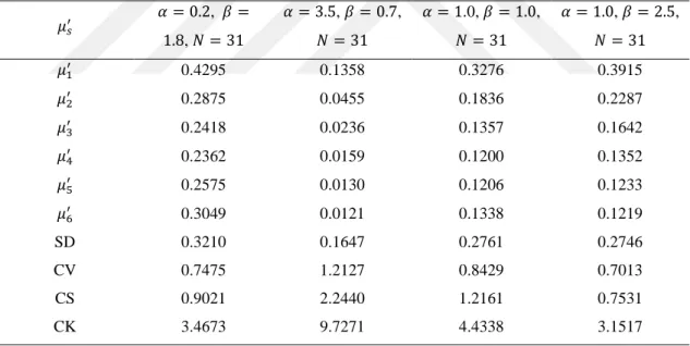
Table 2.3. Moments of ChW distribution for selected parameter values; 𝜆 = 1.5 and 𝛿 = 1. 𝜇𝑠′ 𝛼 = 0.2, 𝛽 = 1.8, 𝑁 = 31 𝛼 = 3.5, 𝛽 = 0.7, 𝑁 = 31 𝛼 = 1.0, 𝛽 = 1.0, 𝑁 = 31 𝛼 = 1.0, 𝛽 = 2.5, 𝑁 = 31 𝜇1′ 0.4295 0.1358 0.3276 0.3915 𝜇2′ 0.2875 0.0455 0.1836 0.2287 𝜇3′ 0.2418 0.0236 0.1357 0.1642 𝜇4′ 0.2362 0.0159 0.1200 0.1352 𝜇5′ 0.2575 0.0130 0.1206 0.1233 𝜇6′ 0.3049 0.0121 0.1338 0.1219 SD 0.3210 0.1647 0.2761 0.2746 CV 0.7475 1.2127 0.8429 0.7013 CS 0.9021 2.2440 1.2161 0.7531 CK 3.4673 9.7271 4.4338 3.1517
2.6. Maximum Likelihood Estimation of ChW Distribution
Let 𝑋1, 𝑋2, … , 𝑋𝑛 be a random sample from ChW distribution and 𝝍 = (𝜆, 𝛿, 𝛼, 𝛽) be the parameter vector. The likelihood and log-likelihood functions for ChW distribution are, respectively, given by 𝐿(𝝍|𝒙) = ∏ 𝑓𝐶ℎ𝑊(𝝍, 𝑥𝒊) 𝑛 𝑖=1 = ∏[(ℎ𝐶ℎ(𝑥𝑖) + ℎ𝑊(𝑥𝑖))𝑅𝐶ℎ(𝑥𝑖)𝑅𝑊(𝑥𝑖)] 𝑛 𝑖=1 , (2.6.1) and log 𝐿 (𝝍) = ∑ log(ℎ𝐶ℎ(𝑥𝑖) + ℎ𝑊(𝑥𝑖)) 𝑛 𝑖=1 + ∑ log 𝑅𝐶ℎ(𝑥𝑖) 𝑛 𝑖=1 + ∑ log 𝑅𝑊(𝑥𝑖) 𝑛 𝑖=1 (2.6.2) = ∑ log(ℎ𝐶ℎ(𝑥𝑖) + ℎ𝑊(𝑥𝑖)) 𝑛 𝑖=1 + 𝜆 ∑(1 − 𝑒𝑥𝑖𝛿) 𝑛 𝑖=1 − 𝛼 ∑ 𝑥𝑖𝛽 𝑛 𝑖=1 , (2.6.3)
where 𝑥𝑖’s are the observed values of 𝑋𝑖. The log-likelihood function can be derived with respect to 𝜆, 𝛿, 𝛼 and 𝛽 for obtaining the likelihood equations are as follows:
𝜕 log 𝐿 𝜕 𝜆 = ∑ 𝜕ℎ𝐶ℎ(𝑥𝑖) 𝜕𝜆 ℎ𝐶ℎ(𝑥𝑖) + ℎ𝑊(𝑥𝑖) 𝑛 𝑖=1 + ∑ 𝜕𝑅𝐶ℎ(𝑥𝑖) 𝜕𝜆 𝑅𝐶ℎ(𝑥𝑖) 𝑛 𝑖=1 = ∑ 𝛿𝑥𝑖 𝛿−1𝑒𝑥𝑖𝛿 𝜆𝛿𝑥𝑖𝛿−1𝑒𝑥𝑖𝛿+ 𝛼𝛽𝑥 𝑖𝛽−1 𝑛 𝑖=1 + ∑(1 − 𝑒𝑥𝑖𝛿) 𝑛 𝑖=1 = 0, (2.6.4) 𝜕 log 𝐿 𝜕 𝛿 = ∑ 𝜕ℎ𝐶ℎ(𝑥𝑖) 𝜕𝛿 ℎ𝐶ℎ(𝑥𝑖) + ℎ𝑊(𝑥𝑖) 𝑛 𝑖=1 + ∑ 𝜕𝑅𝐶ℎ(𝑥𝑖) 𝜕𝛿 𝑅𝐶ℎ(𝑥𝑖) 𝑛 𝑖=1 = ∑𝜆𝑥𝑖 𝛿−1𝑒𝑥𝑖𝛿[1 + 𝛿(1 + 𝑥 𝑖𝛿)ln 𝑥𝑖] 𝜆𝛿𝑥𝑖𝛿−1𝑒𝑥𝑖𝛿+ 𝛼𝛽𝑥 𝑖𝛽−1 𝑛 𝑖=1 + 𝜆 ∑ 𝑥𝑖𝛿𝑒𝑥𝑖 𝛿 ln 𝑥𝑖 𝑛 𝑖=1 = 0, (2.6.5) 𝜕 log 𝐿 𝜕 𝛼 = ∑ 𝜕ℎ𝑊(𝑥𝑖) 𝜕𝛼 ℎ𝐶ℎ(𝑥𝑖) + ℎ𝑊(𝑥𝑖) 𝑛 𝑖=1 + ∑ 𝜕𝑅𝑊(𝑥𝑖) 𝜕𝛼 𝑅𝑊(𝑥𝑖) 𝑛 𝑖=1
= ∑ 𝛽𝑥𝑖 𝛽−1 𝜆𝛿𝑥𝑖𝛿−1𝑒𝑥𝑖𝛿+ 𝛼𝛽𝑥 𝑖𝛽−1 𝑛 𝑖=1 − ∑ 𝑥𝑖𝛽 𝑛 𝑖=1 = 0 (2.6.6) and 𝜕 log 𝐿 𝜕 𝛽 = ∑ 𝜕ℎ𝑊(𝑥𝑖) 𝜕𝛽 ℎ𝐶ℎ(𝑥𝑖) + ℎ𝑊(𝑥𝑖) 𝑛 𝑖=1 + ∑ 𝜕𝑅𝑊(𝑥𝑖) 𝜕𝛽 𝑅𝑊(𝑥𝑖) 𝑛 𝑖=1 = ∑𝛼𝑥𝑖 𝛽−1+ 𝛼𝛽𝑥 𝑖𝛽−1ln 𝑥𝑖 𝜆𝛿𝑥𝑖𝛿−1𝑒𝑥𝑖𝛿+ 𝛼𝛽𝑥 𝑖𝛽−1 𝑛 𝑖=1 − 𝛼 ∑ 𝑥𝑖𝛽ln 𝑥 𝑖 𝑛 𝑖=1 = 0. (2.6.7)
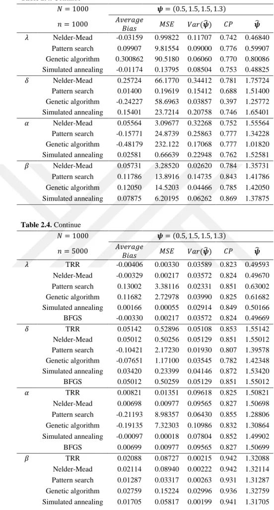
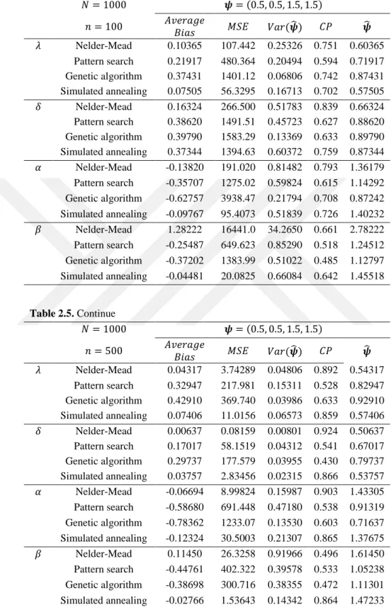
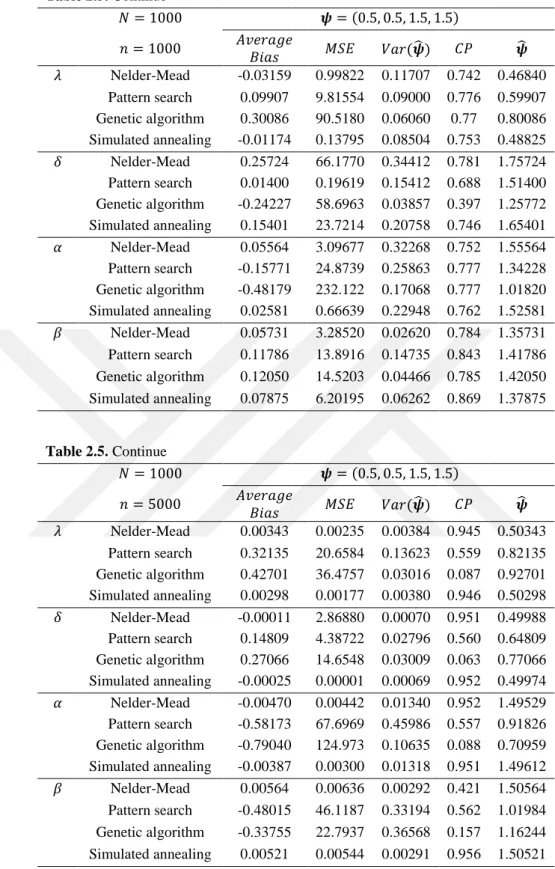
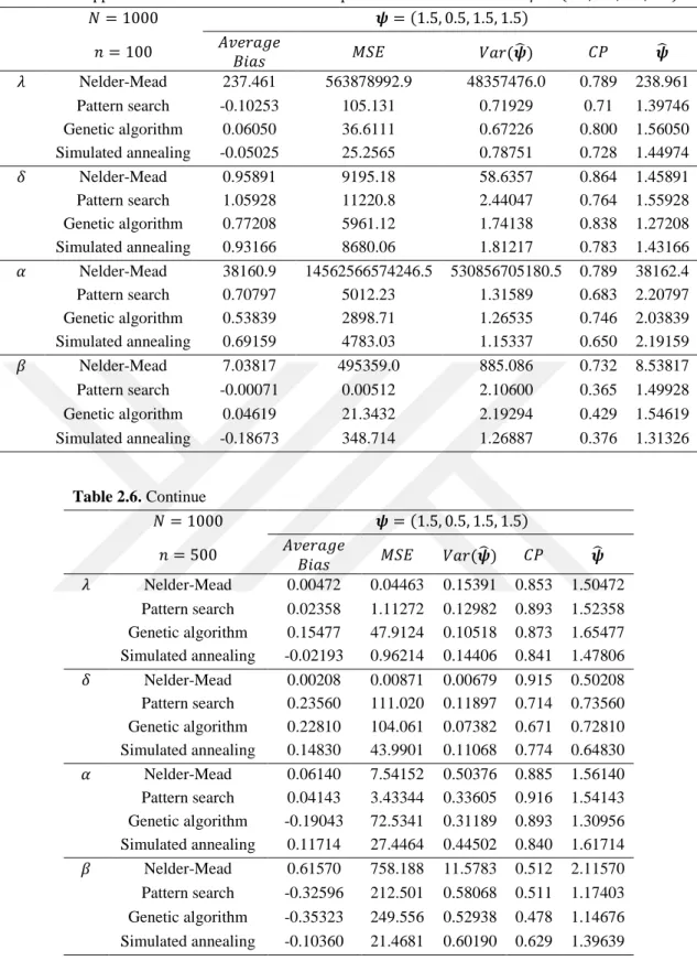
2.7. Monte Carlo Simulation Study
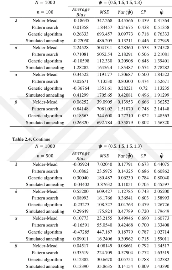
Simulation study is performed to discuss the properties of MLEs. By using Eq. (2.2.1), random data have been generated from ChW distribution. Simulation is conducted with 𝑁 = 1000 trails, sample size 𝑛 = 100, 500, 1000, 5000 and four various values of parameter 𝝍. Tables 2.4-2.7 show all the obtained results such as bias, mean square error (MSE), variance, coverage probability (CP) and mean. Some numerical methods such as BFGS algorithm [36], Nelder-Mead algorithm (fminsearch) [37], Pattern search [38], simulated annealing algorithm (simulannealbnd) [39], genetic algorithm (ga) [40] and sequential quadratic programming (SQP) method or Trust Region Reflective algorithm (TRR) which has been conducted in minimizing method (fmincon) which is described in [41] and [42], all of these algorithms and methods are, separately, used to find the approximations of interest in Tables 2.4-2.7. From these tables, it can be concluded that for getting best results the sample size must be greater than 1000. It is also concluded that simulated annealing algorithm is the best numerical method for estimating the parameters.
Table 2.4. Approximated measures at various sample sizes with 𝑁 = 1000 & 𝜓 = (0.5, 1.5, 1.5, 1.3) 𝑁 = 1000 𝝍 = (0.5, 1.5, 1.5, 1.3) 𝑛 = 100 𝐴𝑣𝑒𝑟𝑎𝑔𝑒 𝐵𝑖𝑎𝑠 𝑀𝑆𝐸 𝑉𝑎𝑟(𝝍̂ ) 𝐶𝑃 𝝍̂ 𝜆 Nelder-Mead -0.18635 347.268 0.45566 0.439 0.31364 Pattern search 0.01358 1.84457 0.24675 0.438 0.51358 Genetic algorithm 0.26333 693.457 0.09773 0.718 0.76333 Simulated annealing -0.22050 486.205 0.13211 0.446 0.27949 𝛿 Nelder-Mead 2.24528 50413.1 8.28360 0.533 3.74528 Pattern search 0.71081 5052.54 2.18291 0.506 2.21081 Genetic algorithm -0.10598 112.330 0.20908 0.648 1.39401 Simulated annealing 1.28282 16456.4 1.85487 0.574 2.78282 𝛼 Nelder-Mead 0.34522 1191.77 1.30687 0.500 1.84522 Pattern search 0.02671 7.13530 0.80300 0.474 1.52671 Genetic algorithm -0.36764 1351.61 0.28221 0.72 1.13235 Simulated annealing 0.41299 1705.65 0.42081 0.496 1.91299 𝛽 Nelder-Mead 0.06252 39.0905 0.13953 0.666 1.36252 Pattern search 0.84148 7081.02 1.51070 0.748 2.14148 Genetic algorithm 0.18563 344.600 0.27710 0.822 1.48563 Simulated annealing 0.26320 692.784 0.35879 0.802 1.56320 Table 2.4. Continue 𝑁 = 1000 𝝍 = (0.5, 1.5, 1.5, 1.3) 𝑛 = 500 𝐴𝑣𝑒𝑟𝑎𝑔𝑒 𝐵𝑖𝑎𝑠 𝑀𝑆𝐸 𝑉𝑎𝑟(𝝍̂ ) 𝐶𝑃 𝝍̂ 𝜆 Nelder-Mead -0.05924 7.02040 0.17791 0.673 0.44075 Pattern search 0.10862 23.5975 0.14325 0.686 0.60862 Genetic algorithm 0.30040 180.487 0.06230 0.784 0.80040 Simulated annealing -0.04402 3.87632 0.11051 0.705 0.45597 𝛿 Nelder-Mead 0.55200 609.427 1.12785 0.743 2.05200 Pattern search 0.08993 16.1766 0.36541 0.603 1.58993 Genetic algorithm -0.23273 108.327 0.04763 0.479 1.26726 Simulated annealing 0.29649 175.824 0.47789 0.720 1.79649 𝛼 Nelder-Mead 0.10773 23.2155 0.49946 0.690 1.60773 Pattern search -0.16591 55.0540 0.42468 0.700 1.33408 Genetic algorithm -0.47285 447.187 0.18779 0.787 1.02714 Simulated annealing 0.09011 16.2406 0.30962 0.715 1.59011 𝛽 Nelder-Mead 0.04517 4.08149 0.08661 0.792 1.34517 Pattern search 0.33519 224.709 0.57904 0.772 1.63519 Genetic algorithm 0.12382 30.6670 0.05754 0.788 1.42382 Simulated annealing 0.13390 35.8635 0.14154 0.809 1.43390
Table 2.4. Continue 𝑁 = 1000 𝝍 = (0.5, 1.5, 1.5, 1.3) 𝑛 = 1000 𝐴𝑣𝑒𝑟𝑎𝑔𝑒 𝐵𝑖𝑎𝑠 𝑀𝑆𝐸 𝑉𝑎𝑟(𝝍̂ ) 𝐶𝑃 𝝍̂ 𝜆 Nelder-Mead -0.03159 0.99822 0.11707 0.742 0.46840 Pattern search 0.09907 9.81554 0.09000 0.776 0.59907 Genetic algorithm 0.300862 90.5180 0.06060 0.770 0.80086 Simulated annealing -0.01174 0.13795 0.08504 0.753 0.48825 𝛿 Nelder-Mead 0.25724 66.1770 0.34412 0.781 1.75724 Pattern search 0.01400 0.19619 0.15412 0.688 1.51400 Genetic algorithm -0.24227 58.6963 0.03857 0.397 1.25772 Simulated annealing 0.15401 23.7214 0.20758 0.746 1.65401 𝛼 Nelder-Mead 0.05564 3.09677 0.32268 0.752 1.55564 Pattern search -0.15771 24.8739 0.25863 0.777 1.34228 Genetic algorithm -0.48179 232.122 0.17068 0.777 1.01820 Simulated annealing 0.02581 0.66639 0.22948 0.762 1.52581 𝛽 Nelder-Mead 0.05731 3.28520 0.02620 0.784 1.35731 Pattern search 0.11786 13.8916 0.14735 0.843 1.41786 Genetic algorithm 0.12050 14.5203 0.04466 0.785 1.42050 Simulated annealing 0.07875 6.20195 0.06262 0.869 1.37875 Table 2.4. Continue 𝑁 = 1000 𝝍 = (0.5, 1.5, 1.5, 1.3) 𝑛 = 5000 𝐴𝑣𝑒𝑟𝑎𝑔𝑒 𝐵𝑖𝑎𝑠 𝑀𝑆𝐸 𝑉𝑎𝑟(𝝍̂ ) 𝐶𝑃 𝝍̂ 𝜆 TRR -0.00406 0.00330 0.03589 0.823 0.49593 Nelder-Mead -0.00329 0.00217 0.03572 0.824 0.49670 Pattern search 0.13002 3.38116 0.02331 0.851 0.63002 Genetic algorithm 0.11682 2.72978 0.03990 0.825 0.61682 Simulated annealing 0.00166 0.00055 0.02914 0.849 0.50166 BFGS -0.00330 0.00217 0.03572 0.824 0.49669 𝛿 TRR 0.05142 0.52896 0.05108 0.853 1.55142 Nelder-Mead 0.05012 0.50256 0.05129 0.851 1.55012 Pattern search -0.10421 2.17230 0.01930 0.807 1.39578 Genetic algorithm -0.07651 1.17100 0.03545 0.782 1.42348 Simulated annealing 0.03420 0.23399 0.04146 0.872 1.53420 BFGS 0.05012 0.50259 0.05129 0.851 1.55012 𝛼 TRR 0.00821 0.01351 0.09618 0.825 1.50821 Nelder-Mead 0.00698 0.00977 0.09565 0.827 1.50698 Pattern search -0.21193 8.98357 0.06430 0.855 1.28806 Genetic algorithm -0.19135 7.32303 0.10986 0.832 1.30864 Simulated annealing -0.00097 0.00018 0.07804 0.852 1.49902 BFGS 0.00699 0.00977 0.09565 0.827 1.50699 𝛽 TRR 0.02088 0.08727 0.00215 0.942 1.32088 Nelder-Mead 0.02114 0.08940 0.00222 0.942 1.32114 Pattern search 0.01287 0.03317 0.00263 0.931 1.31287 Genetic algorithm 0.02759 0.15224 0.02996 0.936 1.32759 Simulated annealing 0.01705 0.05817 0.00199 0.941 1.31705
BFGS 0.02114 0.08940 0.00222 0.942 1.32114
Table 2.5. Approximated measures at various sample sizes with 𝑁 = 1000 & 𝜓 = (0.5, 0.5, 1.5, 1.5) 𝑁 = 1000 𝝍 = (0.5, 0.5, 1.5, 1.5) 𝑛 = 100 𝐴𝑣𝑒𝑟𝑎𝑔𝑒 𝐵𝑖𝑎𝑠 𝑀𝑆𝐸 𝑉𝑎𝑟(𝝍̂ ) 𝐶𝑃 𝝍̂ 𝜆 Nelder-Mead 0.10365 107.442 0.25326 0.751 0.60365 Pattern search 0.21917 480.364 0.20494 0.594 0.71917 Genetic algorithm 0.37431 1401.12 0.06806 0.742 0.87431 Simulated annealing 0.07505 56.3295 0.16713 0.702 0.57505 𝛿 Nelder-Mead 0.16324 266.500 0.51783 0.839 0.66324 Pattern search 0.38620 1491.51 0.45723 0.627 0.88620 Genetic algorithm 0.39790 1583.29 0.13369 0.633 0.89790 Simulated annealing 0.37344 1394.63 0.60372 0.759 0.87344 𝛼 Nelder-Mead -0.13820 191.020 0.81482 0.793 1.36179 Pattern search -0.35707 1275.02 0.59824 0.615 1.14292 Genetic algorithm -0.62757 3938.47 0.21794 0.708 0.87242 Simulated annealing -0.09767 95.4073 0.51839 0.726 1.40232 𝛽 Nelder-Mead 1.28222 16441.0 34.2650 0.661 2.78222 Pattern search -0.25487 649.623 0.85290 0.518 1.24512 Genetic algorithm -0.37202 1383.99 0.51022 0.485 1.12797 Simulated annealing -0.04481 20.0825 0.66084 0.642 1.45518 Table 2.5. Continue 𝑁 = 1000 𝝍 = (0.5, 0.5, 1.5, 1.5) 𝑛 = 500 𝐴𝑣𝑒𝑟𝑎𝑔𝑒 𝐵𝑖𝑎𝑠 𝑀𝑆𝐸 𝑉𝑎𝑟(𝝍̂ ) 𝐶𝑃 𝝍̂ 𝜆 Nelder-Mead 0.04317 3.74289 0.04806 0.892 0.54317 Pattern search 0.32947 217.981 0.15311 0.528 0.82947 Genetic algorithm 0.42910 369.740 0.03986 0.633 0.92910 Simulated annealing 0.07406 11.0156 0.06573 0.859 0.57406 𝛿 Nelder-Mead 0.00637 0.08159 0.00801 0.924 0.50637 Pattern search 0.17017 58.1519 0.04312 0.541 0.67017 Genetic algorithm 0.29737 177.579 0.03955 0.430 0.79737 Simulated annealing 0.03757 2.83456 0.02315 0.866 0.53757 𝛼 Nelder-Mead -0.06694 8.99824 0.15987 0.903 1.43305 Pattern search -0.58680 691.448 0.47180 0.538 0.91319 Genetic algorithm -0.78362 1233.07 0.13530 0.603 0.71637 Simulated annealing -0.12324 30.5003 0.21307 0.865 1.37675 𝛽 Nelder-Mead 0.11450 26.3258 0.91966 0.496 1.61450 Pattern search -0.44761 402.322 0.39578 0.533 1.05238 Genetic algorithm -0.38698 300.716 0.38355 0.472 1.11301 Simulated annealing -0.02766 1.53643 0.14342 0.864 1.47233
Table 2.5. Continue 𝑁 = 1000 𝝍 = (0.5, 0.5, 1.5, 1.5) 𝑛 = 1000 𝐴𝑣𝑒𝑟𝑎𝑔𝑒 𝐵𝑖𝑎𝑠 𝑀𝑆𝐸 𝑉𝑎𝑟(𝝍̂ ) 𝐶𝑃 𝝍̂ 𝜆 Nelder-Mead -0.03159 0.99822 0.11707 0.742 0.46840 Pattern search 0.09907 9.81554 0.09000 0.776 0.59907 Genetic algorithm 0.30086 90.5180 0.06060 0.77 0.80086 Simulated annealing -0.01174 0.13795 0.08504 0.753 0.48825 𝛿 Nelder-Mead 0.25724 66.1770 0.34412 0.781 1.75724 Pattern search 0.01400 0.19619 0.15412 0.688 1.51400 Genetic algorithm -0.24227 58.6963 0.03857 0.397 1.25772 Simulated annealing 0.15401 23.7214 0.20758 0.746 1.65401 𝛼 Nelder-Mead 0.05564 3.09677 0.32268 0.752 1.55564 Pattern search -0.15771 24.8739 0.25863 0.777 1.34228 Genetic algorithm -0.48179 232.122 0.17068 0.777 1.01820 Simulated annealing 0.02581 0.66639 0.22948 0.762 1.52581 𝛽 Nelder-Mead 0.05731 3.28520 0.02620 0.784 1.35731 Pattern search 0.11786 13.8916 0.14735 0.843 1.41786 Genetic algorithm 0.12050 14.5203 0.04466 0.785 1.42050 Simulated annealing 0.07875 6.20195 0.06262 0.869 1.37875 Table 2.5. Continue 𝑁 = 1000 𝝍 = (0.5, 0.5, 1.5, 1.5) 𝑛 = 5000 𝐴𝑣𝑒𝑟𝑎𝑔𝑒 𝐵𝑖𝑎𝑠 𝑀𝑆𝐸 𝑉𝑎𝑟(𝝍̂ ) 𝐶𝑃 𝝍̂ 𝜆 Nelder-Mead 0.00343 0.00235 0.00384 0.945 0.50343 Pattern search 0.32135 20.6584 0.13623 0.559 0.82135 Genetic algorithm 0.42701 36.4757 0.03016 0.087 0.92701 Simulated annealing 0.00298 0.00177 0.00380 0.946 0.50298 𝛿 Nelder-Mead -0.00011 2.86880 0.00070 0.951 0.49988 Pattern search 0.14809 4.38722 0.02796 0.560 0.64809 Genetic algorithm 0.27066 14.6548 0.03009 0.063 0.77066 Simulated annealing -0.00025 0.00001 0.00069 0.952 0.49974 𝛼 Nelder-Mead -0.00470 0.00442 0.01340 0.952 1.49529 Pattern search -0.58173 67.6969 0.45986 0.557 0.91826 Genetic algorithm -0.79040 124.973 0.10635 0.088 0.70959 Simulated annealing -0.00387 0.00300 0.01318 0.951 1.49612 𝛽 Nelder-Mead 0.00564 0.00636 0.00292 0.421 1.50564 Pattern search -0.48015 46.1187 0.33194 0.562 1.01984 Genetic algorithm -0.33755 22.7937 0.36568 0.157 1.16244 Simulated annealing 0.00521 0.00544 0.00291 0.956 1.50521
Table 2.6. Approximated measures at various sample sizes with 𝑁 = 1000 & 𝜓 = (1.5, 0.5, 1.5, 1.5) 𝑁 = 1000 𝝍 = (1.5, 0.5, 1.5, 1.5) 𝑛 = 100 𝐴𝑣𝑒𝑟𝑎𝑔𝑒 𝐵𝑖𝑎𝑠 𝑀𝑆𝐸 𝑉𝑎𝑟(𝝍̂ ) 𝐶𝑃 𝝍̂ 𝜆 Nelder-Mead 237.461 563878992.9 48357476.0 0.789 238.961 Pattern search -0.10253 105.131 0.71929 0.71 1.39746 Genetic algorithm 0.06050 36.6111 0.67226 0.800 1.56050 Simulated annealing -0.05025 25.2565 0.78751 0.728 1.44974 𝛿 Nelder-Mead 0.95891 9195.18 58.6357 0.864 1.45891 Pattern search 1.05928 11220.8 2.44047 0.764 1.55928 Genetic algorithm 0.77208 5961.12 1.74138 0.838 1.27208 Simulated annealing 0.93166 8680.06 1.81217 0.783 1.43166 𝛼 Nelder-Mead 38160.9 14562566574246.5 530856705180.5 0.789 38162.4 Pattern search 0.70797 5012.23 1.31589 0.683 2.20797 Genetic algorithm 0.53839 2898.71 1.26535 0.746 2.03839 Simulated annealing 0.69159 4783.03 1.15337 0.650 2.19159 𝛽 Nelder-Mead 7.03817 495359.0 885.086 0.732 8.53817 Pattern search -0.00071 0.00512 2.10600 0.365 1.49928 Genetic algorithm 0.04619 21.3432 2.19294 0.429 1.54619 Simulated annealing -0.18673 348.714 1.26887 0.376 1.31326 Table 2.6. Continue 𝑁 = 1000 𝝍 = (1.5, 0.5, 1.5, 1.5) 𝑛 = 500 𝐴𝑣𝑒𝑟𝑎𝑔𝑒 𝐵𝑖𝑎𝑠 𝑀𝑆𝐸 𝑉𝑎𝑟(𝝍̂ ) 𝐶𝑃 𝝍̂ 𝜆 Nelder-Mead 0.00472 0.04463 0.15391 0.853 1.50472 Pattern search 0.02358 1.11272 0.12982 0.893 1.52358 Genetic algorithm 0.15477 47.9124 0.10518 0.873 1.65477 Simulated annealing -0.02193 0.96214 0.14406 0.841 1.47806 𝛿 Nelder-Mead 0.00208 0.00871 0.00679 0.915 0.50208 Pattern search 0.23560 111.020 0.11897 0.714 0.73560 Genetic algorithm 0.22810 104.061 0.07382 0.671 0.72810 Simulated annealing 0.14830 43.9901 0.11068 0.774 0.64830 𝛼 Nelder-Mead 0.06140 7.54152 0.50376 0.885 1.56140 Pattern search 0.04143 3.43344 0.33605 0.916 1.54143 Genetic algorithm -0.19043 72.5341 0.31189 0.893 1.30956 Simulated annealing 0.11714 27.4464 0.44502 0.840 1.61714 𝛽 Nelder-Mead 0.61570 758.188 11.5783 0.512 2.11570 Pattern search -0.32596 212.501 0.58068 0.511 1.17403 Genetic algorithm -0.35323 249.556 0.52938 0.478 1.14676 Simulated annealing -0.10360 21.4681 0.60190 0.629 1.39639
Table 2.6. Continue 𝑁 = 1000 𝝍 = (1.5, 0.5, 1.5, 1.5) 𝑛 = 1000 𝐴𝑣𝑒𝑟𝑎𝑔𝑒 𝐵𝑖𝑎𝑠 𝑀𝑆𝐸 𝑉𝑎𝑟(𝝍̂ ) 𝐶𝑃 𝝍̂ 𝜆 Nelder-Mead -0.00428 0.01841 0.07487 0.900 1.49571 Pattern search 0.04326 1.87379 0.07488 0.910 1.54326 Genetic algorithm 0.14736 21.7370 0.09323 0.830 1.64736 Simulated annealing -0.02690 0.72470 0.06836 0.894 1.47309 𝛿 Nelder-Mead -0.00114 0.00130 0.00148 0.927 0.49885 Pattern search 0.16562 27.4591 0.05557 0.611 0.66562 Genetic algorithm 0.21486 46.2121 0.06216 0.510 0.71486 Simulated annealing 0.05633 3.17703 0.03352 0.827 0.55633 𝛼 Nelder-Mead 0.04194 1.76109 0.23478 0.916 1.54194 Pattern search -0.03575 1.27996 0.18712 0.932 1.46424 Genetic algorithm -0.22472 50.5515 0.28656 0.846 1.27527 Simulated annealing 0.07962 6.34689 0.20975 0.888 1.57962 𝛽 Nelder-Mead 0.19372 37.5675 1.20115 0.401 1.69372 Pattern search -0.32469 105.529 0.39582 0.570 1.17530 Genetic algorithm -0.39297 154.586 0.45564 0.475 1.10702 Simulated annealing -0.06257 3.91951 0.23580 0.785 1.43742 Table 2.6. Continue 𝑁 = 1000 𝝍 = (1.5, 0.5, 1.5, 1.5) 𝑛 = 5000 𝐴𝑣𝑒𝑟𝑎𝑔𝑒 𝐵𝑖𝑎𝑠 𝑀𝑆𝐸 𝑉𝑎𝑟(𝝍̂ ) 𝐶𝑃 𝝍̂ 𝜆 Nelder-Mead -0.00178 0.00063 0.01535 0.940 1.49821 Pattern search 0.05525 0.61096 0.02351 0.870 1.55525 Genetic algorithm 0.16244 5.28094 0.08497 0.399 1.66244 Simulated annealing -0.01373 0.03775 0.01377 0.948 1.48626 𝛿 Nelder-Mead -0.00017 5.82136 0.00028 0.940 0.49982 Pattern search 0.13878 3.85454 0.03891 0.630 0.63878 Genetic algorithm 0.18250 6.66596 0.04526 0.262 0.68250 Simulated annealing 0.00136 0.00037 0.00164 0.943 0.50136 𝛼 Nelder-Mead 0.00994 0.01978 0.04492 0.948 1.50994 Pattern search -0.08878 1.57753 0.05885 0.896 1.41121 Genetic algorithm -0.27946 15.6291 0.25821 0.416 1.22053 Simulated annealing 0.03145 0.19794 0.03934 0.945 1.53145 𝛽 Nelder-Mead 0.01970 0.07771 0.01750 0.331 1.51970 Pattern search -0.34777 24.2033 0.24884 0.612 1.15222 Genetic algorithm -0.38324 29.3924 0.38442 0.409 1.11675 Simulated annealing -0.00386 0.00298 0.02281 0.946 1.49613
Table 2.7. Approximated measures at various sample sizes with 𝑁 = 1000 & 𝜓 = (1.5, 2.0, 0.5, 0.5) 𝑁 = 1000 𝝍 = (1.5, 2.0, 0.5, 0.5) 𝑛 = 100 𝐴𝑣𝑒𝑟𝑎𝑔𝑒 𝐵𝑖𝑎𝑠 𝑀𝑆𝐸 𝑉𝑎𝑟(𝝍̂ ) 𝐶𝑃 𝝍̂ 𝜆 Nelder-Mead 0.02075 4.30708 0.09621 0.954 1.52075 Pattern search -0.50416 2541.80 0.32137 0.484 0.99583 Genetic algorithm -0.14830 219.938 0.18231 0.806 1.35169 Simulated annealing -0.33313 1109.81 0.29503 0.631 1.16686 𝛿 Nelder-Mead 0.25345 642.414 0.47116 0.946 2.25345 Pattern search -0.55546 3085.42 1.17147 0.446 1.44453 Genetic algorithm 0.01783 3.17980 0.66170 0.799 2.01783 Simulated annealing -0.30258 915.583 0.97397 0.619 1.69741 𝛼 Nelder-Mead 0.08864 78.5831 0.08556 0.913 0.58864 Pattern search 0.99628 9925.80 1.17147 0.489 1.49628 Genetic algorithm 0.39382 1550.99 0.41015 0.811 0.89382 Simulated annealing 0.70495 4969.58 0.79129 0.613 1.20495 𝛽 Nelder-Mead 0.03895 15.1761 0.02743 0.930 0.53895 Pattern search 1.48772 22133.3 2.04872 0.452 1.98772 Genetic algorithm 0.60490 3659.15 1.46410 0.779 1.10490 Simulated annealing 1.01503 10303.0 1.96989 0.000 1.51503 Table 2.7. Continue 𝑁 = 1000 𝝍 = (1.5, 2.0, 0.5, 0.5) 𝑛 = 500 𝐴𝑣𝑒𝑟𝑎𝑔𝑒 𝐵𝑖𝑎𝑠 𝑀𝑆𝐸 𝑉𝑎𝑟(𝝍̂ ) 𝐶𝑃 𝝍̂ 𝜆 Nelder-Mead 0.00311 0.01941 0.01208 0.947 1.50311 Pattern search -0.76884 1182.23 0.18195 0.187 0.73115 Genetic algorithm -0.17122 58.6373 0.11801 0.772 1.32877 Simulated annealing -0.28698 164.715 0.20880 0.677 1.21301 𝛿 Nelder-Mead 0.04895 4.79250 0.03199 0.948 2.04895 Pattern search -1.12678 2539.30 0.48681 0.181 0.87321 Genetic algorithm -0.12052 29.0543 0.37048 0.781 1.87947 Simulated annealing -0.40783 332.658 0.49451 0.679 1.59216 𝛼 Nelder-Mead 0.01878 0.70600 0.01195 0.944 0.51878 Pattern search 1.36631 3733.62 0.49121 0.191 1.86631 Genetic algorithm 0.33385 222.921 0.34641 0.753 0.83385 Simulated annealing 0.52917 560.057 0.66179 0.664 1.02917 𝛽 Nelder-Mead 0.00628 0.07893 0.00377 0.914 0.50628 Pattern search 2.13878 9148.77 1.24925 0.191 2.63878 Genetic algorithm 0.52272 546.480 1.22616 0.753 1.02272 Simulated annealing 0.81878 1340.82 1.63662 0.672 1.31878
Table 2.7. Continue 𝑁 = 1000 𝝍 = (1.5, 2.0, 0.5, 0.5) 𝑛 = 1000 𝐴𝑣𝑒𝑟𝑎𝑔𝑒 𝐵𝑖𝑎𝑠 𝑀𝑆𝐸 𝑉𝑎𝑟(𝝍̂ ) 𝐶𝑃 𝝍̂ 𝜆 Nelder-Mead 0.00033 0.00011 0.00626 0.946 1.50033 Pattern search -0.89654 803.793 0.08535 0.080 0.60345 Genetic algorithm -0.19322 37.3360 0.12080 0.738 1.30677 Simulated annealing -0.12026 14.4626 0.10850 0.838 1.37973 𝛿 Nelder-Mead 0.01768 0.31261 0.01513 0.955 2.01768 Pattern search -1.33736 1788.53 0.21425 0.071 0.66263 Genetic algorithm -0.17586 30.9275 0.38352 0.705 1.82413 Simulated annealing -0.16292 26.5444 0.24840 0.840 1.83707 𝛼 Nelder-Mead 0.00975 0.09511 0.00580 0.956 0.50975 Pattern search 1.57411 2477.84 0.24297 0.077 2.07411 Genetic algorithm 0.35874 128.699 0.36130 0.686 0.85874 Simulated annealing 0.21950 48.1820 0.33388 0.839 0.71950 𝛽 Nelder-Mead 0.00473 0.02238 0.00192 0.859 0.50473 Pattern search 2.44754 5990.49 0.59341 0.076 2.94754 Genetic algorithm 0.58878 346.668 1.33934 0.667 1.08878 Simulated annealing 0.32452 105.317 0.76198 0.836 0.82452 Table 2.7. Continue 𝑁 = 1000 𝝍 = (1.5, 2.0, 0.5, 0.5) 𝑛 = 5000 𝐴𝑣𝑒𝑟𝑎𝑔𝑒 𝐵𝑖𝑎𝑠 𝑀𝑆𝐸 𝑉𝑎𝑟(𝝍̂ ) 𝐶𝑃 𝝍̂ 𝜆 Nelder-Mead -0.00093 0.00017 0.00116 0.951 1.49906 Pattern search -0.98873 195.598 0.00106 - 0.51126 Genetic algorithm -0.19088 7.29052 0.11455 0.632 1.30911 Simulated annealing -0.00098 0.00019 0.00115 0.952 1.49901 𝛿 Nelder-Mead 0.00146 0.00043 0.00289 0.949 2.00146 Pattern search -1.47894 437.628 0.00044 - 0.52105 Genetic algorithm -0.18329 6.72219 0.35547 0.515 1.81670 Simulated annealing 0.00157 0.00049 0.00288 0.947 2.00157 𝛼 Nelder-Mead 0.00080 0.00013 0.00117 0.942 0.50080 Pattern search 1.72342 594.273 0.00489 - 2.22342 Genetic algorithm 0.34380 23.6492 0.35025 0.475 0.84380 Simulated annealing 0.00089 0.00016 0.00116 0.943 0.50089 𝛽 Nelder-Mead 0.00027 1.54819 0.00040 0.575 0.50027 Pattern search 2.65589 1411.31 0.01232 - 3.15589 Genetic algorithm 0.56524 63.9252 1.28544 0.496 1.06524 Simulated annealing 0.000324 2.10608 0.00039 0.943 0.50032
Simulation study is also performed to obtained estimated Mean, Std Error, Bias and MSE of MLEs in Rfor (𝜆 = 0.1, 𝛿 = 15, 𝛼 = 0.5, 𝛽 = 20). The results are given in Fig. 2.8. From this figure, it is observed the MSEs and bias are decrease to zero as expected. But
it should be point out that these schemes can be seen for some suitable parameters cases. The estimates are not satisfactory and are also unexpected for some selected parameters.