PROPERTY VALUE ASSESSMENT USING ARTIFICIAL NEURAL NETWORKS, HEDONIC REGRESSION AND NEAREST NEIGHBORS REGRESSION METHODS
Hasan YILDIRIM
Statistics, Kamil Özdağ Faculty of Science, Karamanoğlu Mehmetbey University, Karaman, Turkey [email protected]
(Geliş/Received: 09.07.2018; Kabul/Accepted in Revised Form: 22.01.2019)
ABSTRACT: In this paper, hedonic regression, nearest neighbors regression and artificial neural networks methods are applied to the real and up to date estate data set belongs to Adana province of Turkey. Traditionally, hedonic regression methods have been used to predict house prices. Because of the nature of the relationships between the factors affecting house prices are generally being nonlinear; some alternative methods have been needed. Nearest neighbors regression (k-nn) and artificial neural networks (ANN) present both flexible and nonlinear fittings. Classical hedonic approach and its nonlinear alternatives have been employed on a mixed types data set and compared based on some performance measures including root mean squared error, the coefficient of determination (R squared), the coefficient of determination, and mean absolute error. Cross validation method has been used to determine the appropriate model parameters for nearest neighbors and ANN. According to the results, ANN is found better when compared to other methods in terms of all measures. Besides, k-nn regression method provides reasonable results despite of lower performance than hedonic regression method. It has been seen that ANN is a powerful tool for predicting house prices.
Key Words: Artificial neural networks, Hedonic regression, Housing prices, Nearest neighbors regression, Turkey
Yapay Sinir Ağları, Hedonik Regresyon Ve En Yakın Komşuluk Regresyon Metotlarını Kullanarak Emlak Fiyatlarının Belirlenmesi
ÖZ: Bu çalışmada hedonik regresyon, en yakın komşu regresyon ve yapay sinir ağları metotları Türkiye’nin Adana iline ait gerçek ve güncel bir veri seti üzerinde uygulanmıştır. Geleneksel olarak, ev fiyatlarının tahmininde hedonic regresyon metotları kullanılmaktadır. Ev fiyatlarını etkileyen faktörler arasındaki ilişkilerin yapısının genel olarak doğrusal olmaması nedeniyle bazı alternatif metotlara ihtiyaç duyulmaktadır. En yakın komşuluk regresyon ve yapay sinir ağları hem esnek hem de doğrusal olmayan uyumlar sunmaktadır. Klasik hedonic regresyon yaklaşımı ve doğrusal olmayan alternatifleri karma yapıda ki bir veri kümesine uygulanmış ve hata kareler ortalaması, belirleyicilik katsayısı (R kare) ve ortalama mutlak hatayı içeren bazı performans ölçütlerine dayanarak karşılaştırılmıştır.En yakın komşu ve yapay sinir ağları için uygun model parametrelerini belirlemek için çapraz geçerlilik metodu kullanılmıştır.Sonuçlara göre, yapay sinir ağları diğer metotlarla karşılaştırıldığında tüm ölçülere göre daha iyi bulunmuştur.Ayrıca en yakın komşu metodu hedonik regresyon metodundan daha düşük performanslı olmasına rağmen makul sonuçlar sağlamaktadır. Yapay sinir ağlarının ev fiyatlarının tahmininde güçlü bir araç olduğu görülmüştür.
Anahtar Kelimeler: En yakın komşuluk regresyon, Ev fiyatları, Hedonic regresyon, Yapay sinir ağları, Türkiye
INTRODUCTION
Traditionally, having a house has been one of the main goals of a human being and placed at the central to the entire life. One reason of this situation is that a house has been met the need of shelter
which is the most fundemantal and vital need of us. In other respects, it offers a profitable and wisely investment opportunity. Both being a property and a investment asset, the real estate market has own unique and different characteristics. These characteristics are high cost of supply, heterogenity, durability, locational fixity, the possibility to raise loans against housing collateral, the existence of a well-developed secondary market (Iacoviello, 2000:10; Quigley, 1992 and Miles, 1992).
House market is a composite market inluding many components such as potential owners, building contractors, investors, appraisers, banks, assurers, consultants, market researchers, lenders, developers and so forth (Frew and Jud, 2003; Selim, 2009). As a consequence of this property, a precise and fair estimation of sales price of a house has a particular and great concern. Making mistake on determining the price cause some undesirable results such as increasing or decreasing property tax, excessive profit in favor of some groups or affecting potential houseowners negatively.
Accurately predicting the housing price is not easy and clear problem because of including numerous factors. Structural, locational and enviromental properties of a house affect the price. There is no definite study to choose the exact attributes or properties. A great deal of previous researches have been focused on determining the most important factor on a house price. Several estimation models have been proposed as tools to predict the market price of a house precisely. These models provide some useful insights for understanding individual effects of any attribute on the price. Estimation models were classified into two groups as traditional and advanced by Pagourtzi et al. (2003). In this mentioned study, it was emphasized that models created by assuming an underlying form between the attributes and the prices as traditional. Regression models can be given as example to this kind of models. On the other hand, advanced models are based on mimicking human being. Artificial neural networks, fuzzy logic and ARIMA models are part of advanced methods.
In housing market, hedonic regression methods have been often used. These methods are based on multiple regression except a conceptional differences. The term hedonic refers to “weighting of the relative importance of various components among others in constructing an index of usefulness and desirability” (Goodman, 1998). It originates from microeconomic theory (Lancaster, 1966). While assuming an underlying form between the attributes of a house and the price makes the inference easier, there no clear and obvious way on determining the optimal form. The existing literature on this topic is not so much because of insufficient guidance from economic theory about the proper function (Bin, 2004). Most of the studies focused on estimating the sale price of a house by using some flexible and nonlinear forms which some of them were based on Box-Cox transformation approaches (Box and Cox, 1964). This approach have been aroused interest of researchers and widely used to get better insights. When applying a tranformation on price sounds an attractive option, it is so straightforward and causes many problems on fitting. A notable one is the choice of the proper function. In addition, feature selection is another problem. Problems could be extented as having outliers, nonlinear relationship between attributes and price values, some kind of dependencies, multicollinearity and so on. As a reasonable result of this situation, different approaches have been tried on predicting the housing price. Artificial neural networks and nearest neighbors regression methods have been prefered by the reason of not assuming any underlying functional form between attributes and the price of a house.
Artificial neural networks is a computational and nonlinear statistical modelling method being inspired biological neurons of human beings. It can be used to investigate the relationships between the attributes and price of a house. A neural network basically learns by observing the data itself. Some useful patterns are being searched and used for updating the networks parameters. Some artificial neural networks like multilayer perceptrons (MLP) are being considered as a kind of multiple regression methods because of having structural similarities. Artificial neural networks are parts of non-parametric method by the reason of not assuming any underlying functional form. Nonparametric methods provide more flexible options. A different and well-known member of these methods is nearest neighbors regression method. This method is generally known as k-nearest neighbourhood regression method (k-nn regression). By choosing an optimal k number, it discovers k closest different units to a given one and
uses them to estimate it (James et al., 2013). The value of k is so significant on solution and flexibility of the model.
In this paper, the main goal is to search the efficiencies of k-nn regression method via Gower measure which is a mixed type distance measure, hedonic regression method and artificial neural networks on the property appraising. Additionally, it has been investigated whether the selection of parameters in knn regression and artificial neural networks by using cross validation affect the performance or not. Therefore, causal factors of house prices are being investigated in Adana province of Turkey. Data set has been retrieved from a popular real estate website. Hedonic regression, artificial neural networks and k-nearest neighbors regression methods have been employed and compared with one another. The number of hidden layers and nodes for artificial neural networks and the appropriate k value for k-nn regression are determined via cross validation method. In k-nn regression, Gower distance is employed to calculate the distances and the estimations due to existence of mixed types data set.
This paper is organized as follows. Section 2 shortly reviews the literatures including the aforementioned methods. The details and definitions of hedonic regression, nearest neighbors regression and artificial neural networks are given in Section 3. Section 4 consists of some information about the data set and comparison the results of three methods. Finally conclusions are reported and discussed in Section 5.
RELATED LITERATURE REVIEW
In the literature, most of the studies have been carried out by comparison of several methods which may be useful for predicting house prices. The number and types of attributes are variable. Multiple linear regression, hedonic regression, fuzzy logic, artificial neural networks, memory based reasoning, semi parametric regression methods have been commonly used in these studies. As performance measures, mean squared error, root mean squared error, r squared, mean absolute error, Theil’s U statistic are the preferred measures.
One of the first usage of artificial neural networks (ANN) was carried on the data sets of family residences in England by Borst (1991). Tay and Ho (1992) compared the performance of the back propagation neural network (BP) model and the multiple regression analysis (MRA) model in terms of estimating house sale prices. Similar to Tay and Ho’s study, Worzala et al. (1995) applied ANN to real estate appraisal and compared the results with MRA. In this study, it was found that neural networks were not superior than classical approaches. Rossini (1996) reviewed the literature and used ANN to compare its results with MRE and the actual sale prices. The results in Rossini’s study are variable and there is no single best method. It was aimed to clarify the usage of ANN for estimating sale prices. Cechin et al. (2000) applied multilayer perceptron neural network and ordinary regression analysis to determine an apartment’s monetary worth appraisement at the Porto Alegre city located in Southern Brazil. Neural network was mainly preferred in this study due to the nonlinearity between attributes. Nguyen and Al Cripps (2001) compared ANN and MRA to predict housing prices for single families depending on various data models including the different samples size, the functional forms and the temporal prediction. Some explanations about the usage of ANN and MRA are summaries giving the performance results of comparisons. Limsombunchai and Samarasinghe (2004) compared the predictive power of the hedonic regression model and an artificial neural network model for house price prediction by using a web database in Christchurch, New Zeland. The results of this study suggested to use ANN by emphasize some comments about the black box nature of it and providing variables results in different conditions. Bin (2004) carried out a study including the usage of semi-parametric regression and the comparison with traditional parametric models in terms of prediction performance on housing prices. Semi-parametric regression outperformed the parametric counterparts in this study. Zurada et al. (2006) used fuzzy logic and memory-based reasoning in evaluating residential property values for a real data set and compared them with neural networks and multiple regression. In this study, principal component analysis and variable selection were employed to improve the quality of the results. The
results showed that there was no single superior method for the data set. Khalafallah (2008) used the neural networks based models for predicting house market performance on testing and validation processes. The prediction error was found in the range between -2% and +2% in this study. Selim (2009) applied hedonic regression analysis and ANN to determine the factors of house prices in Turkey. ANN was found a powerful and better alternative than classical hedonic regression in terms of predicting performance. Mousa and Saadeh (2010) built an ANN model for the purpose of automatic appraisal of Jordanian estates to avoid the drawbacks of manual appraisal by using Genetic Algorithm for determining the best networks structure. Some statistical tests were carried out to validate the effectiveness of the proposed method. Kontrimas and Verikas (2011) used the ordinary least squares (OLS), support vector machine (SVM) regression, multilayer perceptron (MLP) and a committee of predictors and compared them. The proposed committee of models outperformed all other predictors. Sampathkumar et al. (2015) applied multiple regression and neural networks for predicting land prices in the state of Tamilnadu, India. The results in this study showed that both models fitted well but neural networks provided better accuracy. Abidoye and Chan (2017) applied ANN for modelling property values in Nigeria and found that ANN could be used as a tool to get reliable and accurate property valuation.
MATERIAL AND METHODS Hedonic Regression Method
As mentioned before, hedonic term is defined as ‘‘the weighting of the relative importance of various components among others in constructing an index of usefulness and desirability” (Goodman, 1998). Hedonic price model indicates that each one of the characteristics of nonhomogenous goods provides different profit or some degree of utility. This model is generally used for determining the fair and accurate price of a good in its market. This approach is originated from the consumer theory developed by Lancaster (1966) and extended to the real estate market by Rosen (1974). The traditional use of hedonic estimation in housing studies has been for the purpose of making inferences about non-observable values of different attributes like air quality, airport noise, commuter access (railway, subway or highway) and neighborhood amenities (Janssen et al., 2001; Selim, 2009). Besides it has been widely used for valuation of agricultural goods, real estate pricing and environmental studies (Limsombunchai and Samarasinghe, 2004).
Multiple regression model has same purpose and usage with hedonic approach. The concept of hedonic can be transfered into regression analysis. The properties of a house refer to the independent variables and the price of a house is the dependent variable. Actually, regression analysis is known as hedonic price model in the real estate or similar markets including valuation of any good (Selim, 2009). Let Y is the dependent variable, X’s are the independent variables and β’s are the individual coefficients for each variable and then the hedonic price model is defined as follows:
𝑌 = β0+ ∑ β𝑖X𝑖 𝑘
𝑖=1
+ 𝜀 (1)
This model is exactly same with multiple linear regression model. However, many different functional forms can be used in this model. The existing literature on this topic is not so much because of that there is insufficient guidance from economic theory about the proper function (Bin, 2004). That’s why there is no obvious and effective way to determine the appropriate form but linear, logarithmic and squared forms have been too often used. The most preferred functional form is the semi logarithmic form because of that it makes possible to interpret every coefficient as being the proportion of a good’s price (Halvorsen andPalmquist, 1980). This basically means that the natural logarithm of the house price is treated as new dependent variable and ordinary least squares approach is applied by using this new
variable. It should be noted that some considerations like outliers, nonlinear relationship between attributes and price values, some kind of dependencies, multicollinearity etc have to be attentively examined in models including some transformations.
Nearest Neighbors Regression Method
Nearest neighbors regression a non-parametric and flexible method which does not assume an underlying functional form for model (James et al., 2013). The conceptional expression of this method is so simple and straightforward when compared to other competitors. It is well-known as k-nearest neighbors regression (k-nn regression) method. The knn approach basically uses the k-closest samples to predict a new unit.
The k-nn regression method can not be defined as a traditional model because of dependency individual samples in data set. In this method, a new sample is predicted by the mean of the k closest neighbors values (Kuhn and Johnson, 2013). Given a new samples, say 𝑥0, and k value, the k-nn
regression discovers the k closest samples to this given sample. When 𝑇0 is defined as the set of this k
samples, the prediction of this new samples is calculated as follows (James et al., 2013): 𝑓̂(𝑥0) =
1 𝑘 ∑ 𝑦𝑖
𝑥𝑖∈𝑇0
(2)
As a measures of this closeness, Euclidean distance is the most commonly used metric in the literature. This metric is defined as follows:
√∑(𝑥𝑚𝑖− 𝑥𝑛𝑖)2 𝑘
𝑖=1
(3)
Here 𝑥𝑚 and 𝑥𝑛 are any two samples in the data set. Minkowski distance measure is generalized
version of Euclidean distance and defined as (Liu, 2007; Kuhn and Johnson, 2013):
√∑|𝑥𝑚𝑖− 𝑥𝑛𝑖|𝑡 𝑘
𝑖=1
𝑡
, 𝑡 > 0 (4)
It can be clearly seen than when t = 2, this metric is equivalent to Euclidean distance. Besides, when t=1, it corresponds to City block distance. City block is generally used to find the distance between binary variables. On the other hand, some popular alternatives like Cosine, Hamming, Jaccard, Tanimoto, Simple Matching measures have been used for different purposes in different contexts and areas. Not only the choice of distance measures but also the scale of the variables is critical in terms of model prediction performance. When the data set includes mixed types of measures, Gower distance can be used to calculate the distances between samples. For this reason, to avoid this potential bias and to make possible each independent variables to contribute equally to the distance, scaling and centering the independent variables is suggested before applying the knn method (Kuhn and Johnson, 2013).
Another consideration is not to have any missing values in data set. If exists, computing the distance between units is impossible. As a tuning parameter, the number of neighbors, k, plays key role on the results. As this value increases, the fit will be less variable and this means that results have high bias but low variance. To get more flexible fit, a smaller K value should be choosen. Inversely to the large value, this creates a model having high variance but low bias. In terms of bias-variance tradeoff, k value should
be determined carefully by using some resampling techniques such as cross-validation (James et al., 2013; Kuhn and Johnson, 2013).
Artificial Neural Networks
Artificial neural networks (ANN) is a computational and nonlinear statistical modelling method being inspired biological neurons of human beings (Bishop, 1995; Kuhn and Johnson, 2013). It has been widely used in many areas such as aerospace, automotive, banking, defense, electronics, entertaintment, financial, insurance, manufacturing, medical, oil and gas, robotics, speech, securities, telecommunications and transportation (Demuth et al., 2014). ANN can also provide accurate predictions in regression context. It can be seen as nonlinear regression methods (Selim, 2009).
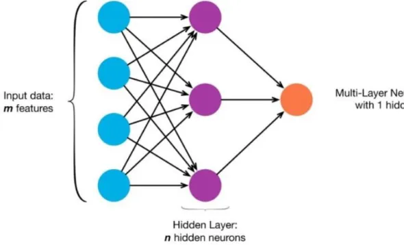
A neural network structure consists of many sub-components such as weights, nodes, layers and activation functions. There are mainly three layers named input layer (includes independent variables values), hidden layer (includes a certain number of processing units, nodes) and the output layer (gives the estimated values of the dependent variable). Weights are generally randomly choosen from a distribution between a determined range values such as [-1,1]. The remain component, activation function produces values by using total net as defined the sum of weighted inputs and the bias values.. All of these components are interconnected with one another. It takes same independent variables as inputs and dependent variable as an output with classical regression models. ANN basically learns by observing the data set itself and updates weights to reduce the error between actual dependent values and estimated ones.
Figure 1. A sample structure of a multilayers neural network (towardsdatascience.com)
The relationship between input and hidden layer can be expressed in linear form and defined as follows:
ht(x) = g (w0+ ∑ xi
P
i=1
wit) (5)
where 𝑔(. ) is the activation function, 𝑤𝑖𝑡 is the weight and 𝑤0 is the bias value between each variable
choosing the number of hidden nodes in hidden layer, the outcome value can be similarly defined as linear combination of this nodes as follows (Kuhn and Johnson, 2013):
f(x) = η0+ ∑ ηt M
t=1
ht (6)
Here 𝑓(𝑥) corresponds to the estimated outcome values. In aANN model, the parameters are updated to minimize or reduce the sum of the squared residuals. This updating process is carried out by using different learning algorithms such as widely used backpropagation algorithm proposed by Rumelhart et al. (1986). It should be noted that there is no guarantee to reach the global optimum solution (Kuhn and Johnson, 2013).
ESTIMATION RESULTS
Data Set, Source and Preprocessing
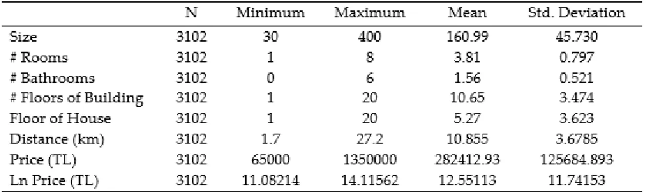
The main data has been retrieved from a well-known real estate website in January and February 2018. It contains 3114 units and 11 variables which are given with some descriptive statistics in Table 2. The data set is belongs to four central districts including Seyhan, Çukurova, Yüreğir and Sarıçam in Adana. The location of house, the age of building, credit availability, size (square meters), the number of rooms, the number of bathrooms, the floor of house, the number of floors of building, the distance to the city central and the heating system of house are used as variables.
Inclusion of outliers may dramatically affect the results. That’s why outlier analysis process is carried out by using some criterias such as studentized residual, leverage values and Cook’s distance. Based on this process, 12 units are omitted from the data set. The results ot outlier analysis is given in Appendix B.
As well as the effect of outliers, multicollinearity is the another important issue because of referring near-linear dependencies between independent variables. The presence of multicollinearity can produce unstable regression coefficients which have large variance/covariances and values in absolute manner (Montgomery et al., 2012). Variance inflation factor and condition index are used to determine whether there is multicollinearity or not. The cutoff values are taken as 10 for Vif and 1000 for CI. There is no multicollinearity between independent variables according to these criterias. The results are given in Appendix C.
The data set is splitted into train and test data. The ratios between them are 70% and 30%, respectively. The models have been fitted by using the training data and tested via testing data. As performance measures RMSE, R squared and MAE have been calculated and given comparatively. The solutions for hedonic regression analysis has been obtained by using IBM Spss and STATA 14.0. The R software has been used for the results of k-nn regression and artificial neural networks.
The descriptive statistics of the data set are given in Table 1 and Table 2. According to descriptive statistics, the majority of the houses are located in Çukurova district. The most of them are at 0-5 years. Combi boilers is the most preferred heating system. The banking credit is available for most houses. There is at a certain amount of dues in almost all houses. The cheapest house price is 65000 (TL) and the maximum price is equal to 1350000 (TL). The mean price is around 282000 (TL)
Table 1. Descriptive statistics (qualitative variables)
Table 2. Descriptive statistics (quantitative variables)
Hedonic Regression Results
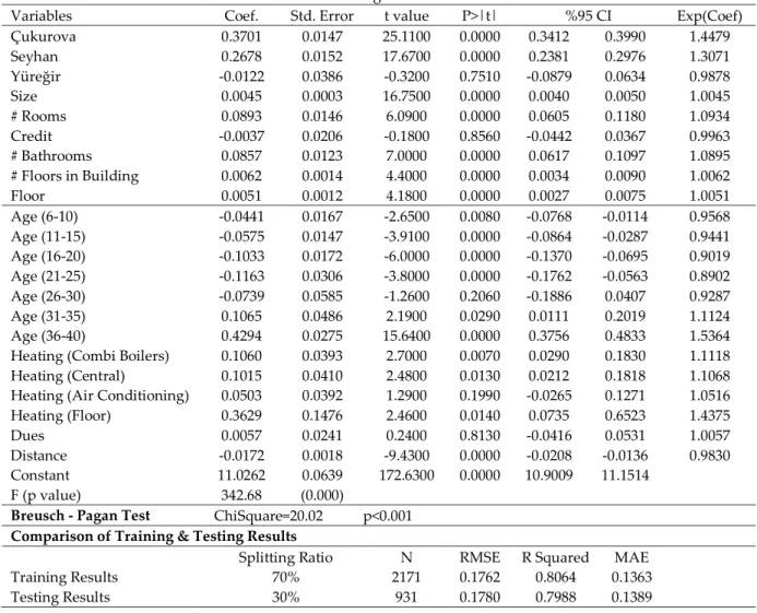
In this section, hedonic regression results are given in Table 3. As mentioned in preprocessing step, there no multicollinearity between independent variables. Another assumption named heteroscedasticity is present when it is checked by Breusch-Pagan test. Robust standart errors for coefficients have been used as a solution to this violation. By doing so, t statistics and p values have been calculated based on these standart errors. The majority of coefficients are significant.
Table 3. Hedonic regression model estimates
Variables Coef. Std. Error t value P>|t| %95 CI Exp(Coef)
Çukurova 0.3701 0.0147 25.1100 0.0000 0.3412 0.3990 1.4479 Seyhan 0.2678 0.0152 17.6700 0.0000 0.2381 0.2976 1.3071 Yüreğir -0.0122 0.0386 -0.3200 0.7510 -0.0879 0.0634 0.9878 Size 0.0045 0.0003 16.7500 0.0000 0.0040 0.0050 1.0045 # Rooms 0.0893 0.0146 6.0900 0.0000 0.0605 0.1180 1.0934 Credit -0.0037 0.0206 -0.1800 0.8560 -0.0442 0.0367 0.9963 # Bathrooms 0.0857 0.0123 7.0000 0.0000 0.0617 0.1097 1.0895 # Floors in Building 0.0062 0.0014 4.4000 0.0000 0.0034 0.0090 1.0062 Floor 0.0051 0.0012 4.1800 0.0000 0.0027 0.0075 1.0051 Age (6-10) -0.0441 0.0167 -2.6500 0.0080 -0.0768 -0.0114 0.9568 Age (11-15) -0.0575 0.0147 -3.9100 0.0000 -0.0864 -0.0287 0.9441 Age (16-20) -0.1033 0.0172 -6.0000 0.0000 -0.1370 -0.0695 0.9019 Age (21-25) -0.1163 0.0306 -3.8000 0.0000 -0.1762 -0.0563 0.8902 Age (26-30) -0.0739 0.0585 -1.2600 0.2060 -0.1886 0.0407 0.9287 Age (31-35) 0.1065 0.0486 2.1900 0.0290 0.0111 0.2019 1.1124 Age (36-40) 0.4294 0.0275 15.6400 0.0000 0.3756 0.4833 1.5364
Heating (Combi Boilers) 0.1060 0.0393 2.7000 0.0070 0.0290 0.1830 1.1118
Heating (Central) 0.1015 0.0410 2.4800 0.0130 0.0212 0.1818 1.1068
Heating (Air Conditioning) 0.0503 0.0392 1.2900 0.1990 -0.0265 0.1271 1.0516
Heating (Floor) 0.3629 0.1476 2.4600 0.0140 0.0735 0.6523 1.4375
Dues 0.0057 0.0241 0.2400 0.8130 -0.0416 0.0531 1.0057
Distance -0.0172 0.0018 -9.4300 0.0000 -0.0208 -0.0136 0.9830
Constant 11.0262 0.0639 172.6300 0.0000 10.9009 11.1514
F (p value) 342.68 (0.000)
Breusch - Pagan Test ChiSquare=20.02 p<0.001
Comparison of Training & Testing Results
Splitting Ratio N RMSE R Squared MAE
Training Results 70% 2171 0.1762 0.8064 0.1363
Testing Results 30% 931 0.1780 0.7988 0.1389
In the last column of hedonic regression results, percent effects (i.e exp(coef)) for each variable are presented. The signs of coefficients and effects are consistent with the literature and expectations. According to these values, the house prices in Çukurova district are higher than Sarıçam (base category) by %44.8. When compared to the prices in Sarıçam, Yüreğir has lower values by %1.2. The results also point out that size, number of rooms, number of bathrooms, number of floors in building have significant and positive effects on the prices.
Age is also an important variable. House prices between 6-10 years are lower than the ones 0-5 years (the based category for age). When age gets older, this difference rises up to 31-35 years. After this age, prices significantly and distinctly increases. This situation ma depend on the places where these houses located. Enviromental and physical conditions may be developed because of being located for a long time. The price of houses having combi boiler as heating system are higher than stove (the base category) by approximately %11. Credit availability, dues, having air conditioning, being 26-30 years and being in Yüreğir district don’t have significant effect on the prices. Observed and predicted house prices for hedonic regression are given in Figure 2.
Figure 2. Observed and predicted house prices by hedonic regression Nearest Neighbors Regression Results
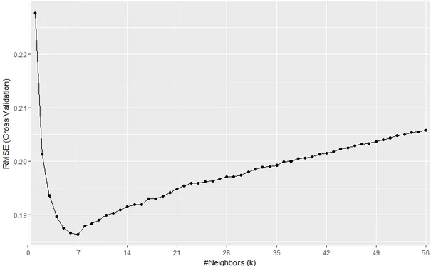
Choosing an optimal k value plays key role on knn regression results. As mentioned before this value should be determined carefully by using some resampling techniques such as cross-validation. In this section, RMSE, Rsquared and MAE performance measures for various k values by using 10 fold - cross validation have been calculated and given in Appendix A. All the results have been carried out by using Gower distance because of having mixed types of measures in our data set. The results can be seen as visually in Figure 3
Both observing Figure 3 and Appendix A, it can be said that as the k value increases, RMSE and MAE values decreases but Rsquared values increases until a certain value. After this value, the change reverses. Herefrom the optimal k value is seen as 7 which is the value providing minimum RMSE, highest Rsquared and reasonable MAE. By using this value, model has been fitted on the whole traning data set. The results for training and testing data are given in Table 4.
Table 4. Nearest neighbors regression results
Splitting Ratio N RMSE Rsquared MAE
Training Results
70% 217
1
0.18481 0.78853 0.13963
Testing Results 30% 931 0.18984 0.77803 0.14505
The results for predicted and observed house prices after fitting k-nn regression is given in Figure 4.
Figure 4. Observed and predicted house prices by k-nn regression Artificial Neural Networks Results
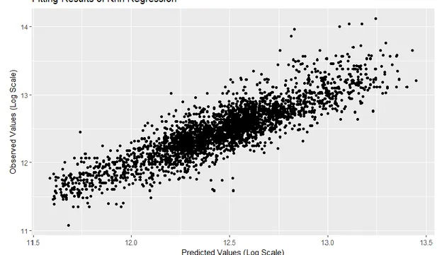
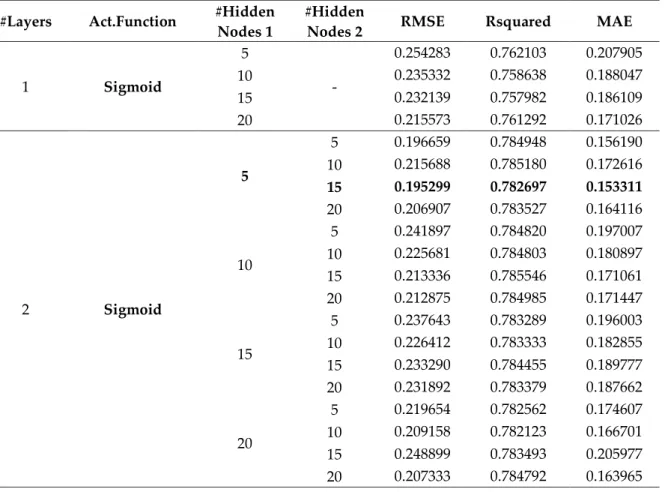
In this study, the number of hidden layers and nodes in each layers are the parameters which must be tuned. Cross validation process has been carried out to determine them effectively. One or two hidden layers options have been considered. As the number of hidden layers nodes {5,10,15,20} values have been tried. Many activation functions have been proposed in the literature. Sigmoid activation function has been most commonly used one and also preferred in this study. RMSE, Rsquared and MAE performance measures have been calculated for every possible combination including one or two hidden layers and four possible number of hidden layer nodes depending on training and testing data sets. According to these results, the best combination has been found when we used sigmoid activation function, five and fifteen hiddens nodes for hidden layer 1 and hidden layer 2, respectively. The minimum testing RMSE value has been calculated for this combination. The results for each combination are given in Table 5. By using these options, the model has been fitted on whole training data set. Testing results have been obtained by using testing data set via this model.
Table 5. Artificial neural networks results #Layers Act.Function #Hidden
Nodes 1
#Hidden
Nodes 2 RMSE Rsquared MAE
1 Sigmoid 5 - 0.254283 0.762103 0.207905 10 0.235332 0.758638 0.188047 15 0.232139 0.757982 0.186109 20 0.215573 0.761292 0.171026 2 Sigmoid 5 5 0.196659 0.784948 0.156190 10 0.215688 0.785180 0.172616 15 0.195299 0.782697 0.153311 20 0.206907 0.783527 0.164116 10 5 0.241897 0.784820 0.197007 10 0.225681 0.784803 0.180897 15 0.213336 0.785546 0.171061 20 0.212875 0.784985 0.171447 15 5 0.237643 0.783289 0.196003 10 0.226412 0.783333 0.182855 15 0.233290 0.784455 0.189777 20 0.231892 0.783379 0.187662 20 5 0.219654 0.782562 0.174607 10 0.209158 0.782123 0.166701 15 0.248899 0.783493 0.205977 20 0.207333 0.784792 0.163965
Table 6. Multilayer perceptron results
Splitting Ratio N RMSE Rsquared MAE
Training Results 70% 2171 0.16605 0.82899 0.13065
Testing Results 30% 931 0.16806 0.83055 0.13037
The results for predicted and observed house prices after fitting multilayer perceptron with two hidden layers and sigmoid activation function are given in Figure 5.
Figure 5. Observed and predicted house prices by multilayer perceptron Comparison of Three Methods
An overall examination of the results is given in Table 7. According to these results, ANN is the best method to predict house prices. It has both the lowest RMSE/MAE values and the highest R squared value. This result suggests that ANN is better tool than Hedonic regression. However, hedonic regression outperforms knn regression in terms of all performance measures. Additionally, the
comparison for prices based on a sample of cases is given in Table 8 and a visual representation of these prices is given in Figure 6.
Table 7. Comparison of test performance of hedonic regression, k-nn regression and ANN Performance Measures Hedonic Regression k-nn
Regression
A NN
Root Mean Squared Error (RMSE) 0.1780 0.1899 0.1
681
R Squared 0.7988 0.7781 0.8
306
Mean Absolute Error (MAE) 0.1389 0.1451 0.1
Table 8. Predicted house prices obtained by hedonic regression, k-nn regression and
ANN
Cases Actual Prices Hedonic Regression Prices k-nn Regression Prices ANN Prices
1 11.65269 11.77351 11.67857 11.64968 2 11.69525 11.78051 11.70286 11.69985 3 11.71994 11.82337 11.94143 11.74309 4 11.60824 11.64289 11.72429 11.58354 5 11.51293 11.56899 11.58000 11.48188 6 11.79056 11.84780 11.74000 11.74497 7 11.63514 11.80945 11.83714 11.69479 8 11.83501 11.79129 11.91286 11.77420 9 11.51293 11.64289 11.72429 11.58354 10 11.50288 11.55723 11.71571 11.42297 11 11.59910 11.48429 11.71286 11.47543 12 11.79810 12.07341 12.07429 11.93719 13 11.38509 11.72688 11.62429 11.64855 14 11.08214 11.50328 11.68000 11.46345 15 12.18075 11.77162 11.79000 11.77241
Figure 6. Actual and predicted prices by hedonic regression, k-nn regression and ANN CONCLUSIONS
In this study, the factors affecting prices of houses which are located in Adana has been investigated by using hedonic regression, nearest neighbors regression and artificial neural networks methods. According to the hedonic regression results, district, age, size, number of rooms, number of bathrooms, type of heating system, floor, number of floors in building, distance to the city center are found as significant variables on the house prices. Because of being flexible and nonlinear alternatives, k nearest neighbourhood and artificial neural networks approaches have been used and compared with hedonic regression. It is shown that the selection of parameters via cross validation in knn regression and ANN is effective on the performance of these methods. Consequently, ANN has been found as the best method
in terms of testing performance on predicting house prices. It can be used as a powerful alternative to ordinary hedonic regression method.
ACKNOWLEDGMENT
The authoris thankful to the associate editor and anonymousreferees for their helpful comments and suggestions during the earlier draft of this paper.
REFERENCES
Abidoye, R. B.,& Chan, A. P., 2017, “Modelling Property Values in Nigeria Using Artificial Neural Network”, Journal of Property Research, 34(1), 36-53.
Bin, O., 2004, “A Prediction Comparison of Housing Sales Prices by Parametric versus Semi-Parametric Regressions”, Journal of Housing Economics, 13(1), 68-84.
Bishop C.,Neural Networks for Pattern Recognition, Oxford University Press, Oxford, 1995.
Borst, R. A., 1991, “Artificial Neural Networks: The Next Modelling/Calibration Technology for the Assessment Community”, Property Tax Journal, 10(1), 69-94.
Box, G.,& Cox, D., 1964, “An Analysis of Transformations”, Journal of the Royal Statistical Society B, 26, 211–252.
Cechin, A., Souto, A. & Gonzalez, M.A., “Real Estate Value at Porto Alegre City Using Ann”, Proceedings 6th Brazilian Symposium On Neural Networks, November, 2000.
Demuth, H. B., Beale, M. H., De Jess, O., & Hagan, M. T., Neural Network Design, Martin Hagan, 2014. Frew, J.,& G. D. Jud., 2003, “Estimating The Value of Apartment Buildings”, The J. Real Estate Res., 25: 77
- 86.
Goodman, A. C., 1998, “Andrew Court and the Invention of Hedonic Price Analysis”, Journal of Urban Economics, 44, 291–298.
Halvorsen, R.,& Palmquist, R., 1980, “The Interpretation of Dummy Variables in Semilogrithmic Regressions”, American Economic Review, 70(June), 474–475.
Iacoviello, M., 2000, “House Prices and the Macroeconomy in Europe: Results from a Structural Var Analysis”, Working Paper Series 0018, European Central Bank.
IBM Corp. Released, 2017, IBM SPSS Statistics for Windows, Version 25.0. Armonk, NY: IBM Corp. James, G., Witten, D., Hastie, T., & Tibshirani, R., 2013, An Introduction to Statistical Learning (Vol. 112).
New York: Springer.
Janssen, C., Söderberg, B., & Zhou, J., 2001, “Robust Estimation of Hedonic Models of Price and Income for Investment Property”, Journal of Property Investment & Finance, 19(4), 342-360.
Khalafallah, A., 2008, “Neural Network Based Model for Predicting Housing Market Performance”, Tsinghua Science & Technology, Vol. 13, Pp. 325-328.
Kontrimas, V.,& Verikas, A., 2011, “The Mass Appraisal of the Real Estate by Computational Intelligence”, Applied Soft Computing, 11(1), 443-448.
Kuhn, M.,& Johnson, K., Applied Predictive Modeling (Vol. 26), New York: Springer, 2013. Lancaster, K. J., 1966, “A new approach to consumer theory”, J .Political Economy, 74:132- 157.
Limsombunchai, V. & Samarasinghe, S., 2004, “House Price Prediction Using Artificial Neural Network: A Comparative Study with Hedonic Price Model”, Applied Economics Journal, Vol. 9-2, Pp. 65-74.
Liu B.,Web Data Mining, Springer, Berlin, Heidelberg, 2017.
Miles, D., 1992, “Housing Markets, Consumption and Financial Liberalisation in the Major Economies”, European Economic Review, 36, 5, 1093- 1127.
Montgomery, D. C., Peck, E. A., & Vining, G. G., Introduction to Linear Regression Analysis (Vol. 821), John Wiley & Sons, 2012.
Mousa, A. A.,& Saadeh, M., 2010, “Automatic Valuation of Jordanian Estates Using A Genetically-Optimised Artificial Neural Network Approach”, WSEAS Transactions on Systems, 9, 905-916. Nguyen, N. & Cripps, A., 2001, “Predicting Housing Value: A Comparison of Multiple Regression
Analysis and Artificial Neural Networks”, The Journal of Real Estate Research, Vol 22 (3): 313-336. Pagourtzi, E., Assimakopoulos, V., Hatzichristos, T., & French, N., 2003, “Real Estate Appraisal: A
Review of Valuation Methods”, Journal of Property Investment & Finance, 21(4), 383-401.
Quigley, J. M., 1992, Housing Markets in J. Eatwell, M. Milgate and P. Newman (eds.), The New Palgrave: A Dictionary of Economics, 3-20, London, Macmillan Press.
R Core Team, 2018, R: A language and environment for statistical computing. R Foundation for Statistical Computing, Vienna, Austria. URL https://www.R-project.org/.
Rosen, S., 1974, “Hedonic Prices and Implicit Markets: Product Differentiation in Pure Competition”, Journal of Political Economy, 82, 34–55.
Rossini, P.A., 1997, “Artificial Neural Networks versus Multiple Regression in the Valuation of Residential Property”, Australian Land Economics Review, November Vol 3(1).
Rumelhart D., Hinton G., & Williams R., Learning Internal Representations by Error Propagation. In Parallel Distributed Processing: Explorations in the Microstructure of Cognition, The MIT Press, 1986. Sampathkumar, V., Santhi, M. H., & Vanjinathan, J., 2015, “Forecasting the Land Price Using Statistical
and Neural Network Software”, Procedia Computer Science, 57, 112-121.
Selim, H., 2009, “Determinants of House Prices in Turkey: Hedonic Regression versus Artificial Neural Network”. Expert Systems with Applications, 36(2), 2843-2852.
StataCorp., 2015, Stata Statistical Software: Release 14, College Station, TX: StataCorp LP. Tay, D. P.,& Ho, D. K., 1992, “Artificial Intelligence and the Mass Appraisal of Residential Apartments”,
Journal of Property Valuation and Investment, 10(2), 525-540.
Worzala, E., Lenk, M., & Silva, A., 1995, “An Exploration of Neural Networks and Its Application to Real Estate Valuation”, Journal of Real Estate Research, 10(2), 185-201.
Zurada, J. M., Levitan, A. S. & Guan, J., 2006, “Non-Conventional Approaches to Property Value Assessment”, Journal of Applied Business Research, Vol. 22(3).
APPENDIX
Appendix A. Performance measures for different k values k RMSE Rsquared MAE k RMSE Rsquared MAE 1 0.22796 0.69301 0.16700 29 0.19714 0.77476 0.14949 2 0.20140 0.74752 0.15054 30 0.19740 0.77483 0.14977 3 0.19353 0.76548 0.14527 31 0.19808 0.77364 0.15035 4 0.18959 0.77448 0.14218 32 0.19850 0.77322 0.15061 5 0.18750 0.78018 0.14109 33 0.19895 0.77303 0.15091 6 0.18659 0.78284 0.14067 34 0.19907 0.77336 0.15100 7 0.18629 0.78420 0.14117 35 0.19924 0.77362 0.15092 8 0.18789 0.78128 0.14263 36 0.19986 0.77254 0.15130 9 0.18833 0.78111 0.14301 37 0.19999 0.77273 0.15143 10 0.18901 0.78026 0.14328 38 0.20045 0.77213 0.15179 11 0.18983 0.77895 0.14364 39 0.20056 0.77253 0.15190 12 0.19028 0.77891 0.14382 40 0.20082 0.77244 0.15222 13 0.19081 0.77845 0.14396 41 0.20132 0.77164 0.15248 14 0.19148 0.77747 0.14419 42 0.20153 0.77143 0.15256 15 0.19188 0.77769 0.14423 43 0.20182 0.77130 0.15283 16 0.19195 0.77843 0.14431 44 0.20228 0.77050 0.15300 17 0.19300 0.77655 0.14506 45 0.20252 0.77039 0.15316 18 0.19307 0.77742 0.14555 46 0.20298 0.76974 0.15348 19 0.19357 0.77694 0.14618 47 0.20323 0.76954 0.15380 20 0.19413 0.77649 0.14652 48 0.20339 0.76957 0.15409 21 0.19472 0.77537 0.14708 49 0.20372 0.76933 0.15429 22 0.19534 0.77468 0.14786 50 0.20406 0.76891 0.15464 23 0.19591 0.77395 0.14826 51 0.20433 0.76880 0.15487 24 0.19593 0.77467 0.14833 52 0.20475 0.76817 0.15521 25 0.19613 0.77455 0.14864 53 0.20502 0.76793 0.15543 26 0.19633 0.77478 0.14878 54 0.20537 0.76729 0.15566 27 0.19665 0.77469 0.14893 55 0.20551 0.76720 0.15580 28 0.19708 0.77429 0.14932 56 0.20580 0.76693 0.15610
Appendix B. The omitted samples and corresponding examination measures Id Rstudent Unadjusted p Value p (Bonferroni) Leverage Values Cook Distance 1 -7,3576 <0.0001 <0.0001 0,152036 0,414871 2 -4,6692 <0.0001 0.00981 0,103549 0,108756 134 -4,4299 <0.0001 0.03031 0,105052 0,099552 358 -4,5360 <0.0001 0.01854 0,062715 0,059481 381 -5,5923 <0.0001 0.00007 0,060364 0,086503 1006 4,3232 <0.0001 0.04926 0,008930 0,007280 1007 7,1096 <0.0001 0.00000 0,022687 0,050210 1137 4,3204 <0.0001 0.04990 0,004876 0,003954 1137 4,3235 <0.0001 0.04918 0,003533 0,002865 1142 4,6071 <0.0001 0.01323 0,009828 0,009101 1548 -4,4388 <0.0001 0.02910 0,010604 0,009126 2299 4,7106 <0.0001 0.00803 0,005806 0,005596 Threshold Values Cook Distance: 4/(𝑛 − 𝑘 − 1) = 0.00129 Leverage: 3𝑝/𝑛 = 0.022158
Studentized Residual:The range of ± 3 Standart Deviation = [−3.00481, 3.00492] Overall Values:
x̅Studentized= 0.000057294
d̅Cook= 0.000453567
xLeverage= 0.00741457
Appendix C. The results of multicollinearity
Variable VIF Dimension Eigenvalues Condition Index
Location 1.333 1 10.540 1.000 Size 5.307 2 0.430 4.949 # of rooms 4.881 3 0.316 5.774 Credit avaliability 1.008 4 0.210 7.076 # of bathrooms 1.500 5 0.172 7.822 # of floors in building 1.280 6 0.110 9.778
The floor of house 1.205 7 0.073 12.057
The age of building 1.605 8 0.057 13.543
Heating system 1.143 9 0.046 15.122
Dues 1.014 10 0.032 18.018