M.Sc. THESIS
December 2018
INTEGRATED NETWORK ROUTING AND SCHEDULING PROBLEM FOR SALT TRUCKS WITH REPLENISHMENT BEFORE SNOWFALL
Thesis Advisor: Assist. Prof. Dr. Gültekin KUYZU
Sorour ZEHTABIYAN
Department of Industrial Engineering
Anabilim Dalı : Herhangi Mühendislik, Bilim Programı : Herhangi Program
ii
Approval of the Graduate School of Science and Technology
……….. Prof. Dr. Osman EROĞUL
Director
I certify that this thesis satisfies all the requirements as a thesis for the degree of Master of Science.
……….
Prof. Dr. Tahir HANALIOĞLU Head of Department
Thesis Advisor : Assist. Prof. Dr. Gültekin KUYZU ... TOBB University of Economics and Technology
Thesis Co-advisor: Assist. Prof. Dr. Eda YÜCEL ... TOBB University of Economics and Technology
Examining Committee Members :
Assist. Prof. Dr Çağrı Koç ... Social Science University of Ankara
The thesis with the title of “Integrated network routing and scheduling problem for salt trucks with replenishment before snowfall” prepared by Sorour Zehtabiyan M.Sc. student of Natural and Applied Sciences institute of TOBB ETU with the student ID 151311010 has been approved on 12.12.2018 by the following examining committee members, after fulfillment of requirements specified by academic regulations.
Assis. Prof. Dr. Ayşegül Altın Kayhan (Chair) ... TOBB University of Economics and Technology
iii
THESIS STATEMENT
Tez içindeki bütün bilgilerin etik davranış ve akademik kurallar çerçevesinde elde edilerek sunulduğunu, alıntı yapılan kaynaklara eksiksiz atıf yapıldığını, referansların tam olarak belirtildiğini ve ayrıca bu tezin TOBB ETÜ Fen Bilimleri Enstitüsü tez yazım kurallarına uygun olarak hazırlandığını bildiririm.
I hereby declare that all the information provided in this thesis was obtained with rules of ethical and academic conduct. I also declare that I have cited all sources used in this document, which is written according to the thesis format of Institute of Natural and Applied Sciences of TOBB ETU.
iv ÖZET
Yüksek Lisans Tezi
KAR YAĞIŞI ÖNCESİNDE TUZ KAMYONLARI İÇİN İKMALLİ ENTEGRE AĞ ROTALAMA VE ÇİZELGELEME PROBLEMİ
Sorour Zehtabiyan
TOBB Ekonomi ve Teknoloji Üniveritesi Fen Bilimleri Enstitüsü
Endüstri Mühendisliği Anabilim Dalı Danışman: Dr.Öğr.Üyesi. Gültekin Kuyzu
Eş Danışman: Dr.Öğr. Eda Yücel Tarih: Aralık 2018
Kar yağışı öncesinde ve sırasında yolların zamanında tuzlanması, trafik güvenliğini iyileştirmek ve trafik sıkışıklığını önlemek için önemli bir önleyici faaliyettir. Bu çalışmada, bir şehir yolu ağındaki tuz kamyonlarının rotalama ve çizelgeleme problemi ele alınmıştır. Ele alınan problem İstanbul Büyükşehir Belediyesinin yoğun kar yağışı durumlarında karşılaştığı bir operasyonel problemdir ve periyodik olarak çözülmelidir. Problemde, araç filosu tuz kapasitesi açısından heterojen araçlardan oluşmaktadır ve birden fazla tuz ikmal noktası bulunmaktadır. Hava şartları gerektirdiğinde, tuzlanması gereken yollar ve bu yollar için öncelik seviyeleri belirlenmektedir. Amaç, ağın farklı noktalarında konumlanmış olan araçların, tuzlanması gereken tüm yolları tuzlayacak şekilde ve yolların ağırlıklı tamamlanma süresini en küçükleyerek rotalanması ve çizelgelenmesidir. Tuza ihtiyacı olan her yol tek bir araç tarafından tuzlanmalıdır. Araçlar tuzlanması gereken bir yolu tuzlama yapmadan sadece geçiş yapmak amacıyla da kullanılabilir. Araçlar, tuzları bittiğinde tuz ikmal noktalarını ziyaret etmelidir. Problemin çözümü için ilk olarak bir karma tam sayılı programlama modeli geliştirilmiştir. Problem büyüklüğü arttıkça modelin performansının hızla düştüğü gözlemlenmiş ve iki aşamalı bir sezgisel yöntem geliştirilmiştir. Sezgiselin ilk aşamasında yapıcı algoritma ile olurlu bir başlangıç çözümü elde edilmektedir, ikinci aşamasında bulunan başlangıç çözümü bir komşuluk arama algoritması ile geliştirilmektedir. Çözüm yaklaşımımızın verimliliği, gerçek hayat yol ağlarını yansıtan rastgele oluşturulmuş örnekler üzerinde analiz edilmiştir. Anahtar Kelimeler: Ayrıt rotalama ve çizelgeleme, Yol tuzlama, Yenileme
v ABSTRACT
Master of Science Thesis
INTEGRATED NETWORK ROUTING AND SCHEDULING PROBLEM FOR
SALT TRUCKS WITH REPLENISHMENT BEFORE SNOWFALL
Sorour Zehtabiyan
TOBB University of Economics and Technology Institute of Natural and Applied Sciences
Department of Industrial Engineering
Advisor: Assist. Prof. Dr. Gültekin Kuyzu
Co-advisor: Assist. Prof. Dr. Eda Yücel
Date: December 2018
Timely salting of roads before the snowfall is an important preventive activity for improving traffic safety and avoiding traffic congestions. We study the problem of routing and scheduling of salt trucks on a city road network. The problem is motivated by the operational problem that the Istanbul Metropolitan Municipality face in case of a heavy snowfall, and thereby should be solved in a periodic manner.In this problem, the vehicle fleet consists of heterogeneous vehicles that differ in salt capacity and there are multiple salt replenishment points. At the beginning of the current planning horizon, given a set of salt needing roads with different urgency levels, the vehicles start from different points of the network (i.e., their final locations at the end of the former planning horizon) and should cover all salt needing roads with the objective of minimizing the total weighted completion time of salting operation of each service needing arc. Each service needing arc should be serviced by exactly one vehicle, however, can be traversed for deadheading by a vehicle as part of its route.Vehicles visit replenishment points when they run out of salt. We first develop a Mixed-Integer Programming model for the problem. Since the performance of the model degrades rapidly as the problem size increases, we propose a simulated annealing metaheuristic, which obtains an initial solution by a constructive heuristic in the first phase, and then improves the solution in the next phase. The efficiency of our solution approach is evaluated on randomly generated instances reflecting real life road networks.
vi
vii
ACKNOWLEDGEMENTS
First I would like to express my sincerest appreciation to my supervisor Dr.Gültekin Kuyzu who made great changes in my academic life by his invaluable insights and supports. I always remind him as the person in the famous proverb who does not give fish to feed people for just one day, he actually teach them how to catch fish and feed them for the life time. He put me in a way that I became convinced about the abilities that I always believed they were impossible for me to do. Besides, by helps of him, I learned outstanding tips in Java which I could not find in any website or course. Second, I acknowledge my co-advisor Dr.Eda Yücel for her nonstop supports and opinions. Her office door was always open for me and I remember the days when she was too busy but she made 3 hours long meeting with me at the middle of her busy day along with her work.
Third, I would like to deeply thank my lovely family members and my boyfriend who always understand me, support me and give me their love without a bit of expectations. Most importantly, I would like to thank my thoughtful brother for always being my supporter and best friend.
Then, I would like to appreciate my jury members that accepted our invitation to attend to my thesis defense and let me know their helpful comments and insights.
I also acknowledge the support of our department’s lovely professors who never let me feel unsupported and disappointed. I especially would like to thank our head of department Dr. Tahir Hanalioğlu who I learned a lot from his science and his life perspective.
Finally I gratefully acknowledge the scholarship received towards my M.Sc. from the TOBB University of Economics and Technology M.Sc. fellowship.
viii
LIST OF FIGURES .... ix
LIST OF TABLES .... x
ABBREVIATIONS .... xi
1. INTRODUCTION .... 1
1.1 Winter Road Maintenance Operations ... 1
1.2 Road Weather Information System ... 2
1.3 Motivation and Contributions ... 3
2. LITERATURE REVIEW .... 5
2.1 Arc routing problems ... 5
2.2 Application of routing problems in WRMO ... 7
3. PROBLEM DESCRIPTION AND MATHEMATICAL MODEL ... 11
3.1 Mathematical formulation ... 14
4. SOLUTION APPROACH .... 19
4.1 Initial solution construction phase ... 19
4.2 Improvement phase: Simulated annealing ... 20
4.3 Parameters of the algorithm ... 21
5. COMPUTATIONAL STUDY .... 23 5.1 Data ... 23 5.2 Scenario Generation ... 26 5.3 Computational Results ... 26 6. CONCLUSION .... 41 REFRENCES .... 42 APPENDIX .... 45 CURRICULUM VITAE ... 50
ix
LIST OF FIGURES
Page Figure 3. 1: Transformation of service needing arcs to service needing nodes ... 14 Figure 3. 2: An illustrative example that demonstrates the transformation of the
original arc routing version of the problem to the node routing version 14 Figure 5. 1 : Districts of Istanbul ... 23
x
LIST OF TABLES
Pages
Table 1.1: Important measurement parameters for weather and route. ... 3
Table 3. 2: Adjacency matrix between all tasks of the network ... 15
Table 5. 1 : Node ID and Population of each district and junction point ... 24
Table 5. 2: Results of MIP and SA for low demands of district (2) ... 29
Table 5. 3: Results of MIP and SA for medium and high demands of district (2) .... 30
Table 5. 4: Results of MIP and SA for low demands of district (3) ... 31
Table 5. 5: Results of MIP and SA for medium and high demands of district (3) .... 32
Table 5. 6: Results of MIP and SA for low demands of district (1-2) ... 33
Table 5. 7: Results of MIP and SA for medium and high demands of district (1-2) . 34 Table 5. 8: Results of MIP and SA for low demands of district (3-6)-a ... 36
Table 5. 9: Results of MIP and SA for low demands of district (3-6)-b ... 37
Table 5. 10: Results of MIP and SA for low demands of district (3-6)-c ... 38 Table 5. 11: Results of MIP and SA for medium and high demands of district (3-6) 39
xi
ABBREVIATIONS
ARP : Arc Routing Problem
CARP : Capacitated Arc Routing Problem
CARPRP : Capacitated Arc routing Problem with Refill Points
CARPRPML : Capacitated Arc routing Problem with Refill Points and Multiple Loads
CCPP : Capacitated Chinese Postman Problem CPP : Chinese Postman Problem
DCC : Disaster Coordination Center DSS : Decision support system GSM : Global System for Mobile
IMM : Istanbul Metropolitan Municipality ILP : Integer Linear Program
ICC : Istanbul Chamber of Commerce MILP : Mixed Integer Linear program RV : Refilling Vehicle
RWIS : Road Weather Information System SA : Simulated Annealing
SV : Service Vehicle
VMS : Variable Message Sign
WRMO : Winter Road Maintenance Operations WRPP : Windy Rural Postman Problem
1 1. INTRODUCTION
The occurrence of extreme weather conditions (rain, fog, or snow) constitute one the most important factors that affects traffic flow in urban areas. Although there might be few heavy precipitations during a year, municipalities should have response plans for severe weather conditions as it has serious effects on human health, social life, and economy.
To the best of our knowledge, there is no recent analysis reporting the economic loss caused by severe weather conditions in Turkey. However, a former research conducted by Istanbul Chamber of Commerce (ICC) in January 2004 estimates that heavy snowfall resulted in an economic loss of approximately 1 billion TL in Istanbul. According to Kadıoğlu et al. (2011), the economic effects of the snowfall can be analyzed under the following main topics:
Disruption in business activities,
Closure of Istanbul Stock Exchange (ISE) and Fluctuation in Monetary transaction,
Loss in foreign trade,
Casualties resulting from traffic accidents, Increase in gasoline consumption,
Tremendous increase in operation cost of, highways, airlines, municipalities.
1.1 Winter Road Maintenance Operations
According to Minsk (1998),the winter road maintenance operations (WRMO) can be categorized as chemical, mechanical, and thermal operations. Chemical operations incorporate solid or liquid freezing point depressant chemicals to melt the ice or prevent its formation. Mechanical approaches such as snow plowing, brooming, and
2
disposing are the operations of collecting loose snow from the surface pavement by pushing it to the sides of the road through blades or collecting and hauling it to the disposal sites if necessary. In the thermal method, heaters are implemented on the surface of the pavement to prevent the formation of bond between the snow and the pavement. The last method is an expensive approach and is mostly used in critical points of big cities such as bridge decks, on and off ramps. These approaches can be used simultaneously in WRMO to increase the efficiency of the operation (Perrier at al. 2007).
According to the starting time of the application of chemicals, the chemical methods are categorized into de-icing and anti-icing approaches. In de-icing methods, the goal is to eliminate the bond of the ice with the pavement surface (after formation of it) and it starts during or after the precipitation by melting snow. On the other hand, in anti-icing methods, the operation is initiated before the formation of bond between the pavement surface and the snow to prevent the formation of the ice. Depending on the condition of road or weather, different chemicals are used in both approaches. Due to its low cost and ease of application, salt is the most prevalent chemical used all around the world. Salt can be combined with abrasives or other solid or liquid chemicals such as calcium chloride in order to enhance its efficacy in temperatures less than -4°C (Boselly et al. 1993). In extreme cold weather situations, there might be some cases when the salt cannot operate properly so pre-wetting is required which is the operation of wetting solid granules before their application in order to increase their effect and prevent them from spreading by the flow of the traffic or wind (Ketcham et al. 1996).
1.2 Road Weather Information System
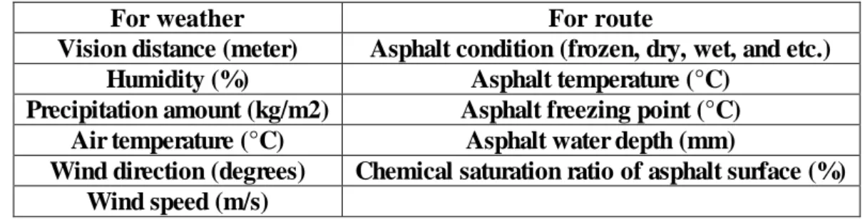
In recent years, by improvements in the technology, Road Weather Information System (RWIS) is used in WRMO. This system is consisting of sensors for forecasting the weather and pavement surface conditions and is installed in critical points of the city. It is designed to help supervisors to take in-time and cost effective decisions by giving information about different weather scenarios. The RWIS in Istanbul cover approximately 5000 kilometers of main routes of the city. The whole system is working unceasingly during 24 hours of a day and it include sensors to get the information about the route and weather conditions of different regions of the city. Its stations are located at 28 different critical locations of the city and cover 4 districts of
3 surface conditions.
Table 1.1: Important measurement parameters for weather and route.
For weather For route
Vision distance (meter) Asphalt condition (frozen, dry, wet, and etc.)
Humidity (%) Asphalt temperature (°C)
Precipitation amount (kg/m2) Asphalt freezing point (°C) Air temperature (°C) Asphalt water depth (mm)
Wind direction (degrees) Chemical saturation ratio of asphalt surface (%) Wind speed (m/s)
The sensors use different energy sources such as solar energy, wind energy, and power energy storage (batteries). They are equipped with GSM technology to send emergency messages to the traffic control center and the disaster control center. In case of emergency, traffic control centers inform motorists through Variable Message Sign (VMS), traffic maps and call centers. Disaster control center take necessary actions to perform winter road maintenance operations. The system includes a decision support system (DSS) to analyze and predict the unfavorable weather conditions as well as the corresponding time and geographical location information. After analyzing data, it will be sent to the relative units of Istanbul Metropolitan Municipality (IMM) in a safe way.
There are totally 1378 vehicles available for winter road maintenance operations. The vehicle fleet used for salt spreading operations consists of trucks, tractors, graders, loaders, Unimogs, and Ategos which have different salt capacities.
To spread salt on the routes, a device should be attached to the tail of the service vehicle. The spread width of the attached device can be adjusted such that a single vehicle with such a device attachment can spread salt up to four lanes width.
1.3 Motivation and Contributions
Motivated by the operational problem that IMM faces with in case of heavy snowfall or cold weather situation, we formulate the problem of routing and scheduling of salting vehicles that are dispatched to service the arcs of the city road network where each arc has a specific urgency level. By getting the advantage of RWIS used in IMM,
4
we suggest a mathematical model and a heuristic approach to determine the routes of salt trucks before an extreme situation. In this approach, by knowing the upcoming weather situation, salting vehicles are dispatched from different points of the network and finish the salting operation within a specific time horizon before the occurrence of extreme situation so there is no need for the extra effort of snow plowing. Furthermore, we propose a heuristic algorithm that outperforms the solution of MIP formulation by solving the problem within few seconds. According to the features of the RWIS that works 24 hours and can send warning messages in every possible time, the proposed approach has a dynamic nature and it can be solved over and over if the urgent situation persists during a day. Furthermore, if the salt amount of the vehicles runs out, they can go to the replenishment points and refill their tanks to continue their service.
There are limited studies in literature considering RWIS in WRMO especially in anti-icing area which aims to use less chemicals in comparison to de-anti-icing method. Therefore, in this study we propose a dynamic approach for routing and scheduling of salting vehicles in anti-icing field.
The remainder of this thesis is organized as follows. In chapter literature review, we review the related works in the literature. In chapter problem description and mathematical model, we define the addressed optimization problem and provide a mathematical formulation for it. In chapter solution approach, we describe the proposed solution approach, which is based on simulated annealing algorithm. In chapter computational study, we present an application of our approach on a set of realistic instances for Istanbul road network. Finally, in chapter conclusion, we summarize our findings.
5 2. LITERATURE REVIEW
In this section we give a brief literature review on Arc Routing Problem (ARP) followed by the implementation of routing problems in the field of WRMO.
2.1 Arc routing problems
ARP, the problem with demands on arcs, is first introduced by Golden et al. (1981) and later different extension problems introduces for it. In ARP if the aim is to find a closed path covering all arcs of the network, the problem becomes Chinese Postman Problem (CPP). However, in some cases, there is no need to cover all arcs of the network; in such cases the problem becomes Rural Postman Problem (RPP) which is the extension of CPP. Furthermore, if a capacity constraint imposed on ARP, it may be referred as Capacitated Arc Routing Problem (CARP). Similarly, Capacitated Chinese Postman Problem (CCPP) is a CPP with capacity constraints.
Amaya et al. (2007) work on the variant of CARP called CARP-RP which considers route markings that should be painted each year and they develop a mathematical model and propose a cutting plane algorithm for it. There are two types of vehicles: service vehicle (SV), that paints the road, and refilling vehicle (RV) which replenish the (SV) when it run out of paint in any point of the network. However, due to the high cost of traversing (RV) on arcs, it is better for (SV) to return to depot when it run out of material. (SV) can paint the central lines of the road segments in both directions however, it should paint the lane separators in the same direction of the corresponding lane. Therefore, the problem is solved on a mixed graph.
Later Amaya et al. (2010) work on the extension of the problem introduced by Amaya et al. (2007) named as capacitated arc routing problem with refill points and multiple loads (CARP-RP-ML). In their procedure, they aim to find a circuit for the (RV) which meets the (SV) multiple times unlike the previous work in which the (RV) should return to depot after each refill process. They aim to simultaneously minimize the total
6
cost of (SV) and (RV) routes and they proposed an Integer Programming formulation and route first and cluster second heuristic procedure for it.
Salazar et al. (2013) give a general formulation for the previous study where the number of servicing vehicles are more than one and they can be refilled either by the refill vehicle or returning to the depot point. They referred to this problem as the synchronized arc and node routing problem problem (SANRP) Which solves two routing problems, multi-vehicle capacitated arc routing problem (for the servicing vehicles), and a node routing problem (for the refilling vehicles). Their objective is to minimize the makespane, i.e., the duration of the longest route and they propose an adaptive large neighborhood search metaheuristic (ALNS) and they test it over a large set of instances.
Laporte et al. (2010) work on a extension of the ARP named as the capacitated arc-routing problem with stochastic demands (CARPSD) for garbage collection problem. They consider the garbage amount on edges of the city network as a decision variable. In the first stage of the problem, they calculate demands by a (ALNS) heuristic. In the next stage they apply the recourse action which is sending vehicles to dump sites when the demand of an arc exceeds the capacity of the vehicle. The ALNS algorithm takes the expected value of the recourse action into account and the objective of the problem is to minimize the total cost of the expected recourse plus the cost of planed solution for the routes of the vehicles which are homogeneous and start from a single depot.
Akbari et al. (2017) study the problem of unblocking the blocked edges after a natural disaster which has made a city network disconnected to fix the network connectivity. They give a Mathematical model and a matheuristic approach for finding the routes and schedule of the vehicles (teams) dispatched to unblock the edges in a synchronized manner in the shortest time. In other words, they consider K-ARCP problems, the combination of arc routing, network design and synchronization concepts in the problems called multi-vehicle synchronized arc routing problem to restore network connectivity.
Nossack et al. (2017) give an extension for windy rural postman problem (WRPP) named as windy rural postman problem with zigzags and time windows (WRPPZTW) and propose two MIP formulation for the problem. They combine two classes of arc routing problems, arc routing problems with time windows, and arc routing problems
7
normal arc routing problems. They also give different number of time windows with different durations in early hours of a day when there is no traffic and show the difficulty level of the WRPPZTM increases dramatically.
2.2 Application of routing problems in WRMO
Similar to problems in other areas of the logistics field, WRMO include decision making in strategic, tactical, operational, and real time levels. Perrier et al. carry out a comprehensive survey on the models and solution approaches of WRMO in all decision levels. In the first part of the survey, they review the problems related to the system design for spreading and snow plowing operations. They also include algorithms and models for partitioning newtork into sectors. In the second part of the survey they involve system design and network partitioning problems for the snow disposal operations. The third part of survey reviews the routing of chemical spreading vehicles and also includes material and vehicle depot location problems. And the forth part covers the routing of snow disposal vehicles beside fleet sizing problems (Perrier et al. 2006, Perrier et al. 2007).
As an early work in CCPP the study of Eglese et al. (1992) is concerned with routing of gritting vehicles by comparing two approaches, normative and prescriptive. The key factor in this study is the concept of routing efficiency which is defined as the proportion of salting distance divided by total distance. In normative approaches, this ratio is a fixed value and is defined based on analysis done on different city road networks. Therefore, normative approach is applied simply to different cases but it has low flexibility in route improvements. However, in the prescriptive approach by solving CCPP for different instances with arbitrary number and location of depots, even the best upper bound solution has less routing efficiency in comparison to normative approach which indicates the important role of network characteristics in the problem which are not taken into account in the normative approach.
Later Li et al (1996) adresses CARP for WRMO. They propose a time constrainted two phase heuristic algorithm for routing of gritting vehicles with additional salt depots under operational constraints of time and capacity to minimize total travelled distance
8
and total number of gritters simultaneously. They impose time constraint by dividing arcs into two categories of precedence. They use the approach of Male et al. (1978) for constructing initial solution by generating a large single tour consisting of arcs which are traversed for deadheading not gritting. Then, during two phases this large tour divided into sub-tours and gritting needing arcs are added to the tours.
Salazar et al. (2018) present a practical study in the field of synchronized snow plowing by proposing a mixed integer formulation and adaptive large neighborhood search heuristic. Synchronization of plowing vehicles that operate on multiple lanes of a same road segment and follow each other is important to prevent the snow mounds at the middle of the routes. To ensure the balance in route duration of vehicles they minimize the makespan of vehicle routes.
Using characteristics of RWIS, Fu et al. (2009) study the problem of real time WRMO and address the dynamic nature of the problem by dividing the time horizon into smaller time intervals and introduce an Integer Linear Program (ILP). Given a certain number of vehicles and a set of pre-specified routes they introduce a decision support model which outputs the schedule of the operation besides what-if analysis for different road weather conditions. Their multi-objective model takes into account service quality and operational costs however, for the sake of simplicity they applied their approach for plowing operation. In our study we try to take the dynamic nature of chemical spreaders into account in anti-icing operation.
Plowing operation initiates when the snow reaches a specific height and might be continued during precipitation. However, in our study thanks to RWIS we assume that the start time of the WRMO is such that the accumulation of the snow on the ground is prevented. Therefore, the gritting operation is carried out without needing for road plowing.
Hajibabai et al. (2014) consider the problem of plowing with priority and salting with replenishment decisions simultaneously. They developed a Mixed Integer Linear program (MILP) with two objective of minimizing total travel time and fuel consumption. Besides, they propose a heuristic algorithm which constructs an initial solution, based on customized 𝐾-mean clustring method and improves it by local perturbations through a customized tabu search approach. Due to the limitation in the maximum road width covered by a snow plower, to model the problem, a road segment
11
3. PROBLEM DESCRIPTION AND MATHEMATICAL MODEL
Similar to the classical CARP, in this problem, we aim to salt a set of streets in a city road network using a fleet of capacity constrained vehicles that should visit replenishment points when their salt tank is empty. Each service needing street can be traversed by more than one vehicle, but only one of these traversals is declared to service the street, all other ones are considered as deadheading. The service needing streets, that is, the streets to be salted, are a small subset of all the streets in the network.
The arc routing problem addressed in this thesis is defined on a directed graph 𝐻 = (𝑉, 𝐸), where the node set 𝑉 = (𝐶 ∪ 𝑅 ∪ 𝐷) is the union of the set of district centers or road junction points (denoted by 𝐶), salt replenishment points (denoted by 𝑅), and depot locations for the vehicles (denoted by 𝐷). The set 𝐸 corresponds to the set of arcs between the nodes in 𝑉. The set 𝑆 𝐸 defines the set of service needing arcs. Each street may have one or more lanes and vehicles can spread salt up to a fixed number of lanes , especially four lanes, on roads during their operational time. The streets with larger number of lanes should be salted more than once or with more than one vehicle depending on the number of lanes. For such streets, the corresponding service needing arc should be copied as much as required to cover the whole number of lanes. Each arc 𝑒 ∈ 𝐸 is associated with a non-negative travelling cost 𝑡𝑒. Each service needing arc 𝑠 ∈ 𝑆 is associated with an urgency level denoted by 𝑤𝑠 and
requires a salt quantity of 𝑞𝑠 and a service time 𝑝𝑠 depending on its number of lanes and length. The service time 𝑝𝑠 of arc 𝑠 ∈ 𝑆 includes the traversal time of the arc, i.e., 𝑝𝑠 ≥ 𝑡𝑠. As salt replenishment requires time, for each node 𝑛 ∈ 𝑅, 𝑝𝑛 denotes the salt
replenishment time, which is assumed to be positive and equal for all vehicles. For any other node 𝑛 ∈ 𝑉 \ 𝑅, the service time is zero, i.e., 𝑝𝑛 = 0.
The heterogeneous vehicle fleet is denoted by the set 𝑀 and each vehicle 𝑣 ∈ 𝑀 has a salt capacity of Qv. At the beginning of the time horizon, which is represented by
(0, 𝑇], vehicle 𝑣 is at depot node 𝑑𝑣 ∈ 𝐷 and is assumed to be full of salt. The ultimate
12
priorities. The service vehicles may run out of salt during the operation, as a result, should visit a replenishment point. A vehicle is allowed to visit a replenishment point although its salt is not completely finished. If a vehicle visits a replenishment point, it is assumed that it leaves the replenishment point full of salt. It is assumed that replenishment points have sufficient amount of chemicals (salt) for any replenishment visit of a vehicle.
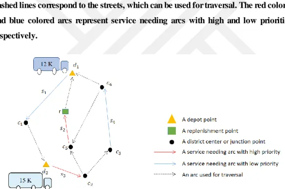
Figure 3. 1illustrates a sample instance of our problem, where 𝑆 is composed of four service needing streets {𝑠1, 𝑠2, 𝑠3, 𝑠4}, 𝐷 is composed of two depots {𝑑1, 𝑑2} for two with salt capacity of 12K and 15K, respectively, 𝑅 is composed of one replenishment point {𝑟}, 𝐶 is composed of 5 district centers or road junction points{𝑐1, 𝑐2, 𝑐3, 𝑐4, 𝑐5}. In the figure, the triangle nodes represent depot points of the vehicles, square nodes represent replenishment points, solid lines represent the service needing streets, and dashed lines correspond to the streets, which can be used for traversal. The red colored and blue colored arcs represent service needing arcs with high and low priorities, respectively.
Figure 3. 1: An illustrative example for the original arc routing version of the problem
Depending on demand locations on the network, there are two main classes in vehicle routing problems, which are node routing and arc routing. In a node routing problem which is first introduced by Dantzig et al. (1959), demands are on nodes of the network whereas demands of an arc routing problem are on arcs. This is commonly used for vehicle scheduling problems in cases such as mail delivery, solid waste, and street
13
demand structure, a common approach in the literature is transforming CARPs to node routing problems (Foulds et al. 2015, Pearn et al. 1987, Tagmouti et al. 2007, Nossack et al. 2017). Below we provide the transformed node routing problem for the original CARP addressed in this study.
The corresponding node routing problem is defined on a complete directed graph 𝐺 = (𝑁, 𝐴) where the node set 𝑁 = (𝑆 ∪ 𝑅 ∪ 𝐷) is the union of the set of service needing arcs (tasks) (𝑆), the set of salt replenishment points (𝑅), and the set of vehicle depot locations (𝐷). The set 𝐴 corresponds to the set of arcs between each pair of nodes in 𝑁. Based on the above notation, each node 𝑖 ∈ 𝑁 is associated with a service time 𝑝𝑖, an urgency level 𝑤𝑖 (where 𝑤𝑖 = 0, for all 𝑖 ∈ (𝑅 ∪ 𝐷), and a demand quantity 𝑞𝑖
(where 𝑞𝑖 = 0, for all 𝑖 ∈ (𝑅 ∪ 𝐷)). The traveling time associated with arc (𝑖, 𝑗) ∈ 𝐴 is denoted by 𝑡𝑖𝑗 and should be calculated as the shortest traveling time from node 𝑖 ∈ (𝑆 ∪ 𝑅 ∪ 𝐷) to node 𝑗 ∈ (𝑆 ∪ 𝑅 ∪ 𝐷) in the original network. As the original arc routing network is connected, the transformed node routing network is complete, i.e., there is a directed arc between each pair of nodes in the network. To find the shortest path between all pairs of nodes, the all pair shortest path algorithm of Floyd-Warshall can be used (Floyd 1962, Warshall 1962).
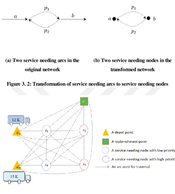
Suppose that there are two service needing arcs 𝑎 and 𝑏 in the original network, and 𝑝1 and 𝑝2 correspond to the shortest paths from the end point of arc 𝑎 to the starting point of arc 𝑏 and from the end point of arc 𝑏 to the starting point of arc 𝑎, with traveling times 𝑡𝑝1 and 𝑡𝑝2, respectively, as shown in Figure 3. 2 (a) After the transformation, the transformed node routing network has two service needing nodes 𝑎 and 𝑏 and two arcs 𝑝1 and 𝑝2 between nodes 𝑎 and 𝑏 with traveling times 𝑡𝑝1 and
𝑡𝑝2, respectively, as shown in Figure 3. 2 (b).
Figure 3. 3 demonstrates the transformed node routing version of the original arc routing version of the problem instance provided in Error! Reference source not found.. In Figure 3. 3 , we have a node for each service needing arc, depot node and replenishment node in Figure 3. 1.
14 (a) Two service needing arcs in the
original network
(b) Two service needing nodes in the transformed network
Figure 3. 2: Transformation of service needing arcs to service needing nodes
Figure 3. 3: The node routing version of the problem instance provided in Figure 3. 1
The notation used throughout the thesis document is provided in Appendix Table 1: Notation.
3.1 Mathematical formulation
For the sake of simplicity in modeling, we generated adjacency sets 𝐼𝑛(𝑖) and 𝑂𝑢𝑡(𝑖) for each node 𝑖 ∈ 𝑁, where 𝐼𝑛(𝑖) denotes the set of all nodes that can be visited just before node 𝑖 ∈ 𝑁 and 𝑂𝑢𝑡(𝑖) denotes the set of all nodes that can be visited just after node 𝑖 ∈ 𝑁.
15
Vehicles are not allowed to go back to their depots or other depots, Vehicles should terminate their routes at a dummy node 𝒆,
Vehicles cannot visit two replenishment nodes consecutively,
Vehicles first might visit replenishment points, just after starting their routes due to the service in the previous time horizon. However, in this thesis we solve the problem for a single time horizon.
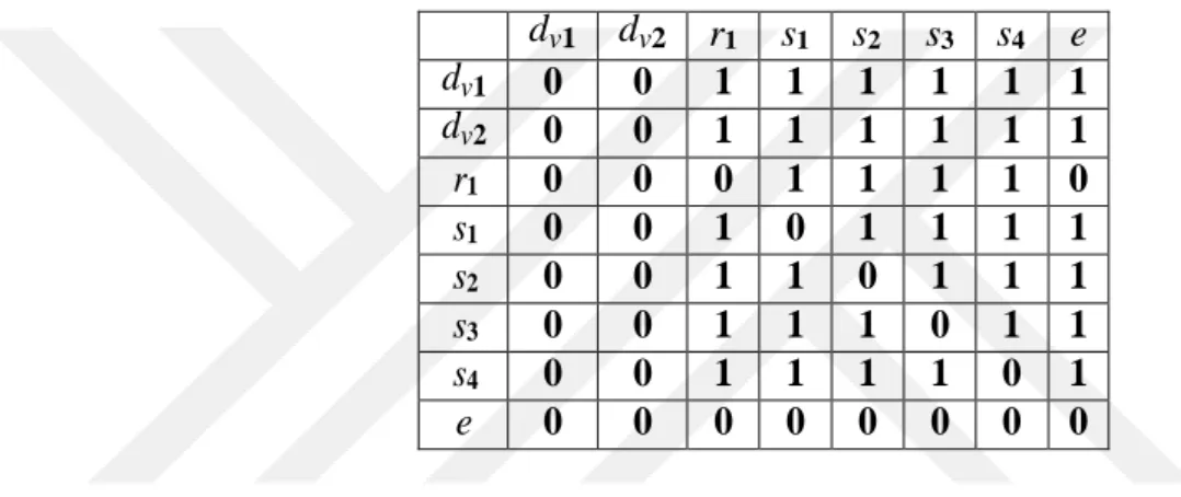
Table 3. 1: Adjacency matrix between all tasks of the network dv1 dv2 r1 s1 s2 s3 s4 e dv1 0 0 1 1 1 1 1 1 dv2 0 0 1 1 1 1 1 1 r1 0 0 0 1 1 1 1 0 s1 0 0 1 0 1 1 1 1 s2 0 0 1 1 0 1 1 1 s3 0 0 1 1 1 0 1 1 s4 0 0 1 1 1 1 0 1 e 0 0 0 0 0 0 0 0
As an illustration Table 3. 1is the adjacency matrix for a network with two depots {𝑑𝑣1, 𝑑𝑣2} (two vehicles), a replenishment point {𝑟1}, and four service needing tasks
{𝑠1, 𝑠2, 𝑠3, 𝑠4}. The corresponding inbound adjacancy set of task 𝑠2 is the set {𝑑𝑣1, 𝑑𝑣2, 𝑟1, 𝑠1, 𝑠3, 𝑠4} and its outbound adjacancy set is the set {𝑟1, 𝑠1, 𝑠3, 𝑠4, 𝑒}. As
shown in the matrix, task 𝑠2 cannot be in the inbound or outbound adjacancy sets of itself and the dummy node e cannot be in the inbound adjacancy set of task 𝑠2.
We can formulate a mixed integer programming model to solve this problem by considering the assumptions listed below:
By solving this problem, the allocation of nodes to the vehicles, sequence of nodes on each vehicle route, and consequently the completion time of each service needing task will be determined. The objective of the problem is to minimize the total weighted completion time of service needing tasks in the time horizon.
We define the decision variables as follows: Let 𝑋𝑖𝑗𝑣 be a binary decision variable, indicating whether vehicle 𝑣 ∈ 𝑀 goes directly from node 𝑖 ∈ 𝑁 to the node 𝑗 ∈ 𝑁 .
16
𝑌𝑖𝑣 is the second binary decision variable, indicating assignment of vehicle 𝑣 ∈ 𝑀 to the node 𝑖 ∈ 𝑁. We define the decision variable ∆𝑖𝑣 for indicating salt level of vehicle 𝑣 ∈ 𝑀 after leaving node 𝑖 ∈ 𝑁. Furthermore, there should be a decision variable for scheduling of vehicles and holding completion time of the tasks; let 𝐶𝑖𝑣 be the completion time of vehicle 𝑣 ∈ 𝑀 after leaving node 𝑖 ∈ 𝑁. We also defined a decision variable for completion time of task 𝑖 ∈ 𝑆 denoted by 𝐵𝑖.
𝑀𝑖𝑛𝑖𝑚𝑖𝑧𝑒 ∑ 𝑊𝑖𝐵𝑖 𝑖∈𝑆 (3.1) Subject to: ∑ 𝑋𝑖𝑗𝑣 𝑗∈𝑂𝑢𝑡(𝑖) = 1 𝑖 = 𝑑𝑣, ∀𝑣 ∈ 𝑀 (3.2) ∑ 𝑋𝑖𝑒𝑣 𝑖∈𝐼𝑛(𝑒) = 1 ∀𝑣 ∈ 𝑀 (3.3) ∑ 𝑋𝑗𝑖𝑣 𝑗∈𝐼𝑛(𝑖) = 𝑌𝑖𝑣 ∀𝑖 ∈ 𝑆 ∪ 𝑅 , ∀𝑣 ∈ 𝑀 (3.4) ∑ 𝑋𝑖ℎ𝑣 𝑖∈𝐼𝑛(ℎ) − ∑ 𝑋ℎ𝑗𝑣 𝑗∈𝑂𝑢𝑡(ℎ) = 0 ∀ℎ ∈ 𝑅 ∪ 𝑆, 𝑣 ∈ 𝑀 (3.5) ∆𝑗𝑣≤ ∆𝑖𝑣− 𝑞𝑗+ 𝑄𝑣(1 − 𝑋𝑖𝑗𝑣) ∆𝑗𝑣≥ ∆𝑖𝑣− 𝑞𝑗− 𝑄𝑣(1 − 𝑋𝑖𝑗𝑣) ∀𝑗 ∈ 𝑆, 𝑖 ∈ 𝐼𝑛(𝑗), 𝑣 ∈ 𝑀 ∀𝑗 ∈ 𝑆, 𝑖 ∈ 𝐼𝑛(𝑗), 𝑣 ∈ 𝑀 (3.6) (3.7) ∆𝑗𝑣= 𝑄𝑣𝑌𝑗𝑣 𝑗 ∈ 𝑅, 𝑣 ∈ 𝑀 (3.8) ∆𝑖𝑣= 𝑄𝑣 𝑖 = 𝑑𝑣 (3.9) 𝐶𝑗𝑣≤ 𝐶𝑖𝑣+ 𝑡𝑖𝑗+ 𝑝𝑗+ 𝐿(1 − 𝑋𝑖𝑗𝑣) 𝐶𝑗𝑣≥ 𝐶𝑖𝑣+ 𝑡𝑖𝑗+ 𝑝𝑗− 𝐿(1 − 𝑋𝑖𝑗𝑣) ∀𝑗 ∈ 𝑆 ∪ 𝑅, 𝑖 ∈ 𝐼𝑛(𝑗), 𝑣 ∈ 𝑀 ∀𝑗 ∈ 𝑆 ∪ 𝑅, 𝑖 ∈ 𝐼𝑛(𝑗), 𝑣 ∈ 𝑀 (3.10) (3.11) 𝐶𝑖𝑣= 0 𝑖 = 𝑑𝑣 , ∀𝑣 ∈ 𝑀 (3.12) 𝐶𝑖𝑣≤ 𝑇 𝑌𝑖𝑣 ∀𝑖 ∈ 𝑆 , ∀𝑣 ∈ 𝑀 (3.13) 𝑍𝑖+ ∑ 𝑌𝑖𝑣 𝑣∈𝑉 = 1 ∀𝑖 ∈ 𝑆 (3.14) 𝐶𝑖𝑣+ 𝜏𝑍𝑖𝑣≤ 𝐵𝑖 ∀𝑖 ∈ 𝑆 , ∀𝑣 ∈ 𝑀 (3.15) 𝑍𝑖, 𝑋𝑖𝑗𝑣, 𝑌𝑖𝑣∈ {0,1} ∀𝑖 ∈ 𝑆 (3.16) ∆𝑖𝑣, 𝐶𝑖𝑣, 𝐵𝑖≥ 0 ∀𝑖 ∈ 𝑁, 𝑣 ∈ 𝑀 (3.17)
In the mathematical formulation, the objective function (3.1) minimizes the total weighted completion time of salting operation of service needing tasks. (3.2) ensures that each vehicle starts it route from their depot. (3.3) ensures that the route of each vehicle terminates at the dummy node 𝑒. (3.4) defines the relation between the decision
17
vehicles from the nodes visited based on the travel times and the time spent at each node, where 𝐿is a sufficiently large number. (3.12) sets the departure time of vehicles from depot to zero. (3.13) ensures that nodes arevisited within the planning horizon. In order to avoid infeasibility, the model allows not to cover some of the service needing tasks within the current planning horizon through (3.13). The estimated completion time of the tasks that are not served with the current planning horizon is set to 𝜏 through (3.15). In our analysis, we set 𝜏 to 3𝑇/2. Constraints (16) and (17) are integrality and non-negativity constraints of the decision variables, respectively.
19 4. SOLUTION APPROACH
The experiments on the mathematical model show that given a limited time the performance of the model degrades rapidly as the problem size increases. Therefore, we propose a heuristic approach in order to obtain good solutions within a tolerable time. The proposed heuristic has two phases. In the first phase, an initial solution is constructed through a constructive heuristic and in the second phase, the initial solution is improved through a simulated annealing (SA) algorithm.
SA is an iterative approach that starts with an initial solution. At each iteration, SA picks a random neighbor from the neighborhood of the current solution with the aim of escaping from the local optima by accepting bad neighbors with a specific probability. It was first modeled by Metropolis et al. (1953) for simulating the annealing of solids. Later, Kirkpatrick et al. (1983) suggest that it can be used in optimization problems as well and since then, it has been widely used in solving combinatorial optimization problems (Kuo et al. 2010, Damodaran et al. 2012, Baños et al. 2013). The name of the algorithm comes from the analogy of its procedure with the annealing process in metallurgy. In process of annealing, the metal with a random crystal structure is heated to the melting temperature and cooled gradually to reach its ground state with minimum thermodynamic free energy. Therefore, in addition to constructing an initial solution, there are four main algorithm-specific decisions to be taken in developing a SA algorithm; Choosing an initial temperature to start the algorithm from, having a random neighboring solution generator structure, specifying bad move acceptance criteria and having a proper cooling schedule. The initial solution construction phase of the proposed approach is described in Appendix Algorithm. 1and SA phase with algorithm-specific decisions are provided in Appendix Algorithm. 2.
4.1 Initial solution construction phase
We construct an initial solution through a two-step greedy approach. In the first step, the service needing tasks are sorted in non-increasing order of their weights multiplied
20
by their processing times, i.e., 𝑤𝑖 𝑝𝑖. In the second step, starting from the first task in the sorted list, the tasks are inserted at the end of the route of the best matching vehicle. For a service needing task 𝑠 ∈ 𝑆, the best matching vehicle, say 𝑣𝑠, is selected among
the set of potential vehicles say 𝑀𝑠, as follows. All vehicles which can serve the task at the end of their current route within the planning horizon, form the set of potential vehicles 𝑀𝑠. The completion time of the task if it were inserted at the end of the current route of each potential vehicle, i.e. 𝐶𝑠𝑣, is calculated, ensuring that the nearest
replenishment point is inserted at the end of the route of the vehicle just before the task if the vehicle does not have enough salt to serve the task. The best matching vehicle, say 𝑣𝑠∗, for the service needing task 𝑠 is a potential vehicle that would complete the
task the earliest, i.e., 𝑣𝑠∗ = argmin
𝑣∈𝑀𝑠{𝐶𝑠
𝑣}.
4.2 Improvement phase: Simulated annealing
In SA, the probability of accepting improving neighbors equals to one whereas the probability of accepting a non-improving neighbor solution 𝑛 of the current solution 𝑐 is denoted by 𝑃(𝑛, 𝑐) and 𝑃(𝑛, 𝑐) is calculated based on Boltzmann distribution provided in 4.1 , where 𝑇 is the temperature of the current state, ∆𝐸 corresponds to the change in the objective function (energy level) of the problem by moving from solution 𝑐 to solution 𝑛, and 𝑘 is the Boltzmann constant that relates temperature to energy:
𝑃(𝑛, 𝑐) = 1 − exp (−∆𝐸 𝑘𝑇)
(4.1)
In the proposed approach, a non-improving solution 𝑛 is accepted if the probability 𝑃(𝑛, 𝑐) is greater than a randomly generated number from the standard uniform distribution. According to Equation 4.1 at higher values of 𝑇, the probability of accepting non-improving neighbor solutions increases. As 𝑇 tends to zero, the probability of accepting non-improving neighbor solutions decreases. In a typical SA optimization, 𝑇 starts high and is gradually decreased according to an annealing schedule 𝑟, that is, at the end of each iteration the new temperature 𝑇′ is calculated as 𝑇’ = 𝑟 𝑇. The annealing schedule should be slow enough to let the algorithm explore the neighborhood. At the beginning of the algorithm there might be some random
21
exchange, transfer, and insert. In swap move, two service needing tasks in the route of a randomly selected vehicle are swapped. In exchange move, two randomly selected service needing tasks in the routes of two different vehicles are exchanged. In transfer move, a randomly selected service needing task is removed from its current route and is inserted into a randomly selected position of the route of a randomly selected vehicle. In insert move, a randomly selected unserved service needing task is inserted into a randomly selected position of the route of a randomly selected vehicle.
We apply a three-step fix operation to each neighbor solution. During the fix operation, first, the replenishment point visits are removed from the routes of the vehicles. Second, starting from the first service needing task of each vehicle, the visited tasks of each vehicle are traversed in the visiting order and a replenishment point visit is inserted between two service needing tasks if the vehicle has enough capacity to cover the salt demand of the former task but it cannot cover the salt demand of the latter one. Third, the service needing tasks that are completed at a time later than 𝑇 are removed from the vehicles they are assigned to. The process of feasibility checks on the new task list is elaborated as a flow chart in Appendix flowchart 1.
4.3 Parameters of the algorithm
According to the equation 4.1 by choosing high values for the starting temperature, the probability of accepting bad moves increases. In order to explore the neighborhood thoroughly, we set the initial temperature equal to 1000. After executing four different move types in each iteration, we calculate the objective function for each move, and finally choose the best move type for that iteration. It is worth noting that if the value of objective function remains unchanged for more than 10 consecutive iterations, we allow the algorithm to take a random worse move. We continue this procedure by slowly decreasing the initial temperature according to the cooling schedule 𝑇’ = 𝑟 𝑇, until the stopping criteria is satisfied. The cooling rate 𝑟 is equal to 0.999 and the stopping criteria in our problem is reaching the temperature to 0.01.
23 5. COMPUTATIONAL STUDY
5.1 Data
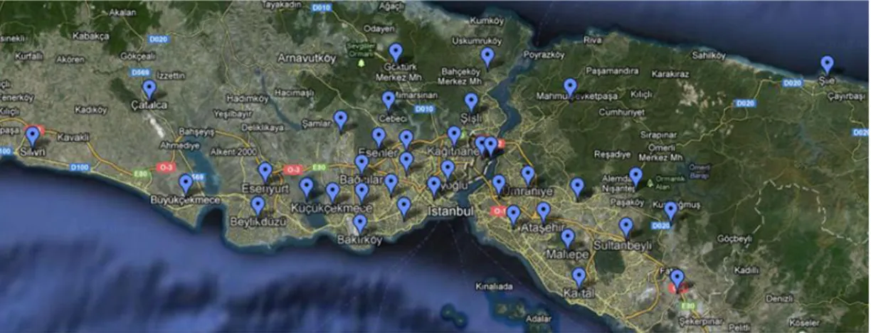
To test the performance of the MIP model and the SA algorithm, we conduct our study on a realistic data set on Istanbul, randomly generated by Yücel et al. (2018). Istanbul is mainly composed of two main motorways in east-west direction and the secondary roads in north-south direction connect these two motorways in junction points in different parts of the city. In order to cover different points of Istanbul, corresponding to each highly populated districts and junction points, nodes are selected. Excluding four low population districts there are 34 nodes for districts and 26 nodes for junction points and we numbers them from 1 to 60. The Figure 5. 1 illustrates the motorways and districts of the Istanbul. As mentioned before, due to the topological features of the network, the path lengths connecting a given node pair (𝑖 and 𝑗) are not the same in both directions of 𝑖 to 𝑗 and 𝑗 to 𝑖. There are 186 arcs connecting 60 nodes directly. According to the location of the nodes, the city is partitioned to 8 regions and for the remainder of this study, we call them districts (which are different from the aformentioned districts of the Istanbul). The Table 5. 1 is the summary of the characteristics of the nodes of the city network nodes.
24
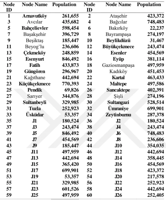
Table 5. 1 : Node ID and Population of each district and junction point
Node ID
Node Name Population Node ID
Node Name Population
1 Arnavutköy 261,655 2 Ataşehir 423,372 3 Avcılar 435,682 4 Bağcılar 748,483 5 Bahçelievler 598,454 6 Bakırköy 22,237 7 Başakşehir 396,729 8 Bayrampaşa 274,197 9 Beşiktaş 185,447 10 Beylikdüzü 31,467 11 Beyog˘lu 236,606 12 Büyükçekmece 243,474 13 Çekmeköy 248,859 14 Esenler 454,569 15 Esenyurt 846,492 16 Eyüp 381,114 17 Fatih 433,873 18 Gaziosmanpaşa 497,959 19 Güngören 296,967 20 Kadıköy 451,453 21 Kağıthane 442,694 22 Kartal 463,433 23 Küçükçekmece 770,393 24 Maltepe 497,586 25 Pendik 69,826 26 Sancaktepe 402,391 27 Sarıyer 344,876 28 Şişli 274,196 29 Sultanbeyli 329,985 30 Sultangazi 528,514 31 Tuzla 252,923 32 Ümraniye 699,901 33 Üsküdar 53,357 34 Zeytinburnu 287,378 35 J1 180,524 36 J2 180,524 37 J3 243,474 38 J4 243,474 39 J5 846,492 40 J6 748,483 41 J7 454,569 42 J8 236,606 43 J9 185,447 44 J10 354,035 45 J11 497,959 46 J12 442,694 47 J13 442,694 48 J14 358,445 49 J15 365,420 50 J16 454,569 51 J17 699,901 52 J18 423,372 53 J19 53,357 54 J20 217,578 55 J21 329,985 56 J22 252,923 57 J23 601,526 58 J24 442,694 59 J25 497,959 60 J26 252,405
Based on the information we obtained from Disaster Coordination Center (DCC), in anti-icing operation, we assume the required amount of salt is equal to 40 𝑔𝑟/𝑚2. To calculate the total demand of an arc, we assume the required salt for gritting is proportional to its length and its number of lanes. We calculate the demand amount of a given arc 𝑖 ∈ 𝑆 by the following formula:
𝑞𝑖 = rate of salt spreading × number of lanes of the route segment ×
25 weight of corresponding salt stored in the tanks.
5𝑚3~12000 kg = 12 tons
7𝑚3~15000 kg = 15 tons
The demand of some arcs of the network might be too high that cannot be serviced completely by a single vehicle with a full tank capacity. In order to overcome this situation, we add dummy nodes at the middle of the arcs with demands greater than the full tank capacity of the smaller vehicle (12 tones).
Based on the surplus demand amount of an arc, we divide it into two or three parts.
In order to give priorities to different service needing arcs of a district, the population of the origin and destination points of the arcs of the district are taken into account.
The weight of a specific service needing arc would be calculated by the following formula:
weight of an arc =population indicator of the service needing arc population indicators of its district
Population indicator of an arc = population of the source
+population of the destination
population indicator of a district =
Sum of population indicators of all arcs of the district (including service needing
arcs and non service needing arcs)
We assume the speed of all vehicles are equal to 70𝑘𝑚
ℎ while they are deadheading on
arcs and we calculate the deadheading time of vehicles by dividing the length of arcs by this speed. We calculate the servicing time of the vehicle (𝑃𝑖) on a given arc 𝑖 ∈ 𝑆
26
40 𝑘𝑚/ℎ. In order to generate all pairs shortest paths matrix between each node pair (𝑖 , 𝑗 ∈ 𝑁), we use traveling time between them (𝑡𝑖𝑗) as the input of Floyd-Warshall algorithm. 𝑃𝑖 = (1 40− 1 70) × arc length 5.2 Scenario Generation
To generate different scenarios, we get the arcs of different districts of the city with different sizes, as to cover different points of the network. Each scenario takes a single district or a combination of two districts into account. In order to get the corresponding arcs of the chosen districts, we look for the arcs with both of their origin and destination points locating in the chosen district. Besides, there might be some arcs, which one of their ends is located in the chosen district but the other end is located in another district, different from the selected one. For the sake of simplicity in our calculations, we do not consider these types of arcs. We specify three different demand levels as low, medium and high for each scenario: The values 30%, 50%, and 75% correspond to the percent of service needing arcs of a chosen district. To generate different instances for each scenario, we randomly choose different arcs of the chosen district and assign demand to them. To this end, we solve the problem starting from the small instances with low number of service needing arcs and increase them up to three levels of low, medium, and high.
5.3 Computational Results
The MIP model and the solution approach is coded in JAVA and compiled on a workstation with two Xeon(R) E5645 processors running at 2.00 GHz and 128 GB of memory.
As the MIP problem is a hard problem, by increasing the number of decision variables it might take hours to solve a problem to optimallity. Therefore, in order to obtain an upper bound on a best possible solution for MIP, we specify a fixed execution time (7200 seconds) as a time limit for the problems with greater sizes. For each instance,
27
the instances with the specific number of service needing arcs, we assign different number of vehicles to service them.
"DST(3-4)-V3R2-11" denotes an instance including both districts 3 and 4 with 3 vehicles and 2 replenishment points and 11 service needing arcs.
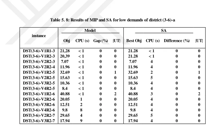
The middle section of each table describes details of the solution obtained from the MIP formulation. The first column of this section is the value of the objective function of the MIP and the second column of the section corresponds to the solution time of the MIP in terms of seconds. The term “Gap” indicates the percentage of the optimality gap of the CPLEX and it is nonzero for the instances, in which the evaluated upperbound and lower bound are not the same value. The notation of “|UT|” in both sections of the table indicates the number of unrouted service needing tasks, the tasks that are not covered in the current time horizon. The columns in the right section of the table correspond to details of the SA algorithm. The “Best Obj” is the best value of the SA algorithm among 15 runs. Similar to the other section, the second column of this section shows the CPU time of the algorithm in terms of seconds. The column under “Difference” heading shows the percentage of the difference between solutions obtained from the MIP and SA algorithm. To illustrate, 0 indicates that the SA algorithm finds the same solution with the MIP’s and a negative value indicates the algorithm finds a better solution.
Table 5. 2 corresponds to the low demand level and Table 5. 3 corresponds to the medium and high demand levels for the service needing arcs of district 2 with total arc number of 14. Similarly, the Table 5. 4corresponds to the low demand level and Table 5. 5 corresponds to the medium and high demand levels of district 3 with total number of 19 arcs. For the low demand levels of the instances that their sum of vehicles, replenishment points and the service needing arcs are less than 9, the MIP solves the problem within 1 second and for the rest of the instances it solves the problem within few seconds. Furthermore, the simulated annealing finds the optimal objective for all of the instances within maximum 5 seconds.
28
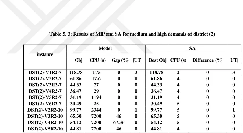
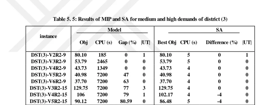
For the medium and high demand levels of the districts, the SA algorithm finds the same solutions found by the MIP formulation within maximum 5 seconds. It is worth noting that in the high demand levels, the MIP formulation cannot solve the problem to optimality within the predefined time limit. However, the SA algorithm finds the MIP’s solution within 5 seconds and in some cases, it gaves better results. (Instances DST(3)-V4R2-15 and DST(3)-V5R2-15 gave better solutions with 4% difference). As shown in the objective values, for all of three demand levels, the instances with unrouted tasks have greater objective values in comparison with the instance, which have the same number of service needing arcs covering all of them. This fact leads us to increase the number of vehicles.
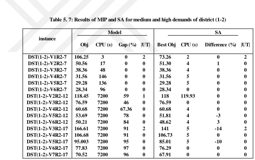
Table 5. 6 and Table 5. 7 correspond to an approximately medium size scenario which is the combination of two districts, 1 and 2 with 24 arcs. Similar to the aforementioned scenarios, the model solves the instances with low and medium demand levels within a short time and the simulated annealing algorithm solves the problem within maximum 4 seconds. Except for one instance of DST(1-2)-V1R1-5 which finds a worse solution with 13.43% difference with the MIP solution, in the rest of instances with medium demand level, the SA finds the same solution with the MIP model. For the high level demands, the MIP finds upperbound solutions with high optimality gaps within 7200 seconds however, the SA algorithm finds the same and in some instance with 14% difference better solutions.
29
instance
Model SA
Obj CPU (s) Gap (%) |UT| Best Obj CPU (s) Difference (%) |UT|
DST(2)-V1R1-3 21.22 < 1 0 0 21.22 2 0 0 DST(2)-V2R1-3 12.39 < 1 0 0 12.39 4 0 0 DST(2)-V3R1-3 11.23 < 1 0 0 11.23 4 0 0 DST(2)-V1R1-4 36.42 < 1 0 1 36.42 2 0 1 DST(2)-V2R1-4 18.52 < 1 0 0 18.52 4 0 0 DST(2)-V3R1-4 14.59 < 1 0 0 14.59 4 0 0 DST(2)-V1R1-5 59.73 < 1 0 1 59.73 2 0 1 DST(2)-V2R2-5 31.50 < 1 0 0 31.80 4 0 0 DST(2)-V3R2-5 24.25 4 0 0 24.25 4 0 0 DST(2)-V4R2-5 20.56 4 0 0 20.56 4 0 0 DST(2)-V1R2-6 91.82 < 1 0 2 91.82 2 0 2 DST(2)-V2R2-6 46.54 4 0 0 46.54 4 0 0 DST(2)-V3R2-6 31.87 9 0 0 31.87 5 0 0 DST(2)-V4R2-6 26.58 16 0 0 26.58 4 0 0 DST(2)-V5R2-6 25.17 39 0 0 25.17 4 0 0
30
Table 5. 3: Results of MIP and SA for medium and high demands of district (2)
instance
Model SA
Obj CPU (s) Gap (%) |UT| Best Obj CPU (s) Difference (%) |UT|
DST(2)-V1R2-7 118.78 1.75 0 3 118.78 2 0 3 DST(2)-V2R2-7 61.86 17.6 0 0 61.86 4 0 0 DST(2)-V3R2-7 44.33 27 0 0 44.33 4 0 0 DST(2)-V4R2-7 36.47 29 0 0 36.47 4 0 0 DST(2)-V5R2-7 31.19 1194 0 0 31.19 4 0 0 DST(2)-V6R2-7 30.49 25 0 0 30.49 5 0 0 DST(2)-V2R2-10 99.77 2344 0 1 99.77 5 0 1 DST(2)-V3R2-10 65.30 7200 46 0 65.30 5 0 0 DST(2)-V4R2-10 54.12 7200 67.36 0 54.12 5 0 0 DST(2)-V5R2-10 44.81 7200 46 0 44.81 4 0 0
31
instance
Model SA
Obj CPU (s) Gap (%) |UT| Best Obj CPU (s) Difference (%) |UT|
DST(3)-V1R1-3 19.86 < 1 0 0 19.86 2 0 0 DST(3)-V2R1-3 13.47 < 1 0 0 13.47 3 0 0 DST(3)-V3R1-3 10.95 < 1 0 0 10.95 3 0 0 DST(3)-V1R1-4 27.82 < 1 0 0 27.82 2 0 0 DST(3)-V2R1-4 16.86 < 1 0 0 16.86 4 0 0 DST(3)-V3R1-4 13.29 < 1 0 0 13.29 2 0 0 DST(3)-V1R1-5 42.77 < 1 0 1 42.77 3 0 1 DST(3)-V2R1-5 20.78 < 1 0 0 20.78 4 0 0 DST(3)-V2R2-5 15.85 3 0 0 15.85 4 0 0 DST(3)-V3R2-5 21.48 3 0 0 21.48 3 0 0 DST(3)-V4R2-5 14.28 2 0 0 14.28 4 0 0 DST(3)-V1R2-6 66.44 < 1 0 1 66.44 2 0 1 DST(3)-V2R2-6 30.70 4 0 0 30.70 4 0 0 DST(3)-V3R2-6 23.59 6 0 0 23.59 4 0 0 DST(3)-V4R2-6 22.03 14 0 0 22.03 4 0 0
32
Table 5. 5: Results of MIP and SA for medium and high demands of district (3)
instance
Model SA
Obj CPU (s) Gap (%) |UT| Best Obj CPU (s) Difference (%) |UT|
DST(3)-V2R2-9 80.10 185 0 1 80.10 5 0 1 DST(3)-V3R2-9 53.79 2465 0 0 53.79 5 0 0 DST(3)-V4R2-9 43.73 1349 0 0 43.73 4 0 0 DST(3)-V5R2-9 40.98 7200 47 0 40.98 4 0 0 DST(3)-V6R2-9 37.70 7200 63 0 37.70 4 0 0 DST(3)-V3R2-15 129.75 7200 77 3 129.75 4 0 0 DST(3)-V4R2-15 106 7200 79 1 102.17 4 -4 0 DST(3)-V5R2-15 90.12 7200 80.59 0 86.48 5 -4 0
33
instance
Obj CPU (s) Gap (%) |UT| Best Obj CPU (s) Difference (%) |UT|
DST(1-2)-V1R1-3 21.5 < 1 0 0 21.5 2 0 0 DST(1-2)-V2R1-3 8.68 < 1 0 0 8.68 3 0 0 DST(1-2)-V3R1-3 7.74 < 1 0 0 7.74 4 0 0 DST(1-2)-V1R1-4 46.04 < 1 0 0 46.04 2 0 0 DST(1-2)-V2R1-4 16.30 < 1 0 0 16.30 4 0 0 DST(1-2)-V3R1-4 15.26 < 1 0 0 15.26 2 0 0 DST(1-2)-V1R1-5 59.9 < 1 0 1 67.95 3 13.43 2 DST(1-2)-V2R1-5 25.7 < 1 0 0 25.7 2 0 0 DST(1-2)-V2R2-5 24.61 < 1 0 0 24.61 4 0 0 DST(1-2)-V3R2-5 21.48 3 0 0 21.48 3 0 0 DST(1-2)-V4R2-5 18.22 5 0 0 18.22 4 0 0 DST(1-2)-V1R2-6 73.26 < 1 0 1 73.26 2 0 1 DST(1-2)-V2R2-6 32.03 4 0 0 32.03 4 0 0 DST(1-2)-V3R2-6 24.49 8 0 0 24.49 4 0 0 DST(1-2)-V4R2-6 20.99 6.73 0 0 20.99 4 0 0 DST(1-2)-V5R2-6 20.28 2 31 0 20.28 4 0 0
34
Table 5. 7: Results of MIP and SA for medium and high demands of district (1-2)
instance
Model SA
Obj CPU (s) Gap (%) |UT| Best Obj CPU (s) Difference (%) |UT|
DST(1-2)-V1R2-7 106.25 3 0 2 73.26 2 0 2 DST(1-2)-V2R2-7 50.56 17 0 0 51.30 4 1 0 DST(1-2)-V3R2-7 38.36 48 0 0 38.36 4 0 0 DST(1-2)-V4R2-7 31.56 146 0 0 31.56 5 0 0 DST(1-2)-V5R2-7 29.28 136 0 0 29.28 5 0 0 DST(1-2)-V6R2-7 28.34 96 0 0 28.34 0 0 0 DST(1-2)-V2R2-12 118.45 7200 59 1 118 119.93 0 0 DST(1-2)-V3R2-12 76.59 7200 46 0 76.59 0 0 0 DST(1-2)-V4R2-12 60.68 7200 67.36 0 60.68 4 0 0 DST(1-2)-V5R2-12 53.69 7200 78 0 51.81 4 -3 0 DST(1-2)-V6R2-12 50.21 7200 84 0 48.62 4 3 0 DST(1-2)-V3R2-17 166.61 7200 91 2 141 5 -14 2 DST(1-2)-V4R2-17 106.68 7200 91 0 106.73 5 0 0 DST(1-2)-V5R2-17 95.003 7200 95 0 85.01 5 -10 0 DST(1-2)-V6R2-17 77.83 7200 97 0 76.29 0 0 0 DST(1-2)-V7R2-17 70.52 7200 96 0 67.91 0 0 0
35
problem and the model and the SA algorithm try to find the nearest replenishment point in case a vehicle runs out of salt.
The tasks orders of vehicles in the solution found by MIP model which finds a suboptimal solution of 166.15 within 7200 seconds is shown below:
{93 , 10 , R1 , 16 , 6 , 26 } {5 , 88 , 14 , 27 , R2 , 15 , 25} {3 , 94 , 11 , 89 , R2 , 17}
Completion time of vehicle 1: 2.60 Completion time of vehicle 2: 2.86 Completion time of vehicle 3: 2.77
According to the first route, the salt level of the first vehicle after servicing two tasks 93 and 10 decreases such that it cannot service the task 16, so it chose the nearest replenishment point (R1) to its current position (task10) and it proceeds toward R1 to refill its tank and after refilling, it continues to service till it does not pass the time horizon. The second and third vehicles similarly run out of salt during their service, but they choose R2 as a nearest replenishment point to go. However, the solution found by SA algorithm which gives lower objective value (141.27) has different task orders for vehicles as demonstrated below.
{93 , 10 , 94 , R1 , 11 , 15} {14 , 27 , 26 , R2 , 17}
{88 , 5 , 16 , R2 , 89 , 6 , 91}
Completion time of vehicle 1: 2.46 Completion time of vehicle 2: 2.11 Completion time of vehicle 3: 2.88
36
Table 5. 8: Results of MIP and SA for low demands of district (3-6)-a
instance
Model SA
Obj CPU (s) Gap (%) |UT| Best Obj CPU (s) Difference (%) |UT|
DST(3-6)-V1R1-3 21,28 < 1 0 0 21.28 < 1 0 0 DST(3-6)-V1R2-3 20,39 < 1 0 0 21.28 < 1 0 0 DST(3-6)-V2R2-3 7.07 < 1 0 0 7.07 4 0 0 DST(3-6)-V2R2-4 11.96 < 1 0 0 11.96 4 0 0 DST(3-6)-V1R2-5 32.69 < 1 0 1 32.69 2 0 1 DST(3-6)-V2R2-5 15.63 < 1 0 0 15.63 5 0 0 DST(3-6)-V3R2-5 10.36 < 1 0 0 10.36 4 0 0 DST(3-6)-V4R2-5 8.4 < 1 0 0 8.4 4 0 0 DST(3-6)-V1R2-6 40.88 < 1 0 2 40.88 3 0 2 DST(3-6)-V2R2-6 20.05 1 0 0 20.05 4 0 0 DST(3-6)-V3R2-6 12.51 2 0 0 12.51 4 0 0 DST(3-6)-V4R2-6 9.8 8 0 0 9.8 4 0 0 DST(3-6)-V2R2-7 29.65 4 0 0 29.65 5 0 0 DST(3-6)-V3R2-7 17.94 9 0 0 17.94 4 0 0
37
instance
Model SA
Obj CPU (s) Gap (%) |UT| Best Obj CPU (s) Difference (%) |UT|
DST(3-6)-V3R2-7 38.36 48 0 0 38.36 4 0 0 DST(3-6)-V4R2-7 14.05 16.34 0 0 14.05 5 0 0 DST(3-6)-V2R2-8 42.02 7 0 1 42.02 5 0 0 DST(3-6)-V3R2-8 24.52 35.77 0 0 24.52 4 0 0 DST(3-6)-V4R2-8 18.83 28 0 0 18.83 4 0 0 DST(3-6)-V5R2-8 16.99 49.59 0 0 18.83 4 10 0 DST(3-6)-V2R2-9 48.16 21 0 1 48.16 6 0 1 DST(3-6)-V3R2-9 28.87 84 0 0 28.87 5 0 0 DST(3-6)-V4R2-9 23.19 75 0 0 23.19 5 0 0 DST(3-6)-V5R2-9 21.34 120 0 0 21.34 5 0 0
38
Table 5. 10: Results of MIP and SA for low demands of district (3-6)-c
instance
Model SA
Obj CPU (s) Gap (%) |UT| Best Obj CPU (s) Difference (%) |UT|
DST(3-6)-V2R2-10 58.34 72 0 1 58.34 5 0 1 DST(3-6)-V3R2-10 33.93 434 0 0 33.93 5 0 0 DST(3-6)-V4R2-10 26.68 708 0 0 26.68 5 0 0 DST(3-6)-V5R2-10 24.84 7200 42 0 24.98 7 0.5 0 DST(3-6)-V2R2-11 64.94 147 0 2 64.94 6 0 2 DST(3-6)-V3R2-11 38.52 1430 0 0 38.52 5 0 0 DST(3-6)-V4R2-11 30.64 2855 0 0 30.64 5 0 0 DST(3-6)-V5R2-11 27.89 7200 65 0 27.88 5 0 0
39
instance
Model SA
Obj CPU (s) Gap (%) |UT| Best Obj CPU (s) Difference (%) |UT|
DST(3-6)-V5R3-18 56.38 7200 88.45 0 54.44 6 -3.4 0 DST(3-6)-V6R3-18 48.45 7200 91 0 46.99 5 -3.01 0 DST(3-6)-V7R3-18 44.26 7200 92 0 43.86 6 -0.9 0 DST(3-6)-V9R3-25 89.65 7200 99 1 72.14 6 -19.53 1 DST(3-6)-V10R3-25 77.91 7200 99 0 68.54 6 -12.02 0 DST(3-6)-V11R3-25 75.34 7200 99 0 63.77 6 -15.35 0 DST(3-6)-V12R3-25 65.70 7200 98 0 61.47 6 -6.43 0