T.R.
SELCUK UNIVERSITY
THE GRADUATE SCHOOL OF NATURAL AND APPLIED SCIENCE
ACCURACY COMPARISON BETWEEN GPS ONLY AND GPS PLUS GLONASS IN RTK AND STATIC
METHODS
Rozh Ismael Abdulmajed ABDULMAJED MASTER THESIS
Department of Geomatics Engineering
December-2017 KONYA All Rights Reserved
iv ABSTRACT MS THESIS
ACCURACY COMPARISON BETWEEN GPS ONLY AND GPS PLUS GLONASS IN RTK AND STATIC
METHODS
Rozh Ismael Abdulmajed ABDULMAJED
THE GRADUATE SCHOOL OF NATURAL AND APPLIED SCIENCE OF SELCUK UNIVERSITY
THE DEGREE OF MASTER, GEOMATICS ENGINEERING
Advisor: Assoc. Prof. Dr. Ramazan Alpay ABBAK 2017, 45 Pages
Jury
Advisor Assoc. Prof. Dr. Ramazan Alpay ABBAK Prof. Dr. Muzaffer KAHVECİ
Assist. Prof. Dr. Hüseyin Zahit SELVİ
Today, with the quick development and changing of the space geodesy and satellite techniques, opportunities for choosing and using GNSS increased, many satellite systems are available and ready to use. Nowadays the direction goes towards combining signals from multiple GNSSs to maintain greater availability, higher performance, especially in the engineering sector while using DGNSS (differential GNSS) for land surveying or mapping like data collection in the field, establishing reference points. At present using DGNSS for different purposes are so common and attracts many users, especially for surveying and mapping applications. Therefore, comparing the use of GPS only and GPS + GLONASS for RTK and static in terms of the position quality is important.
In this study, a detailed information was given about GNSS positioning and its error sources, GPS system and GLONASS system. Differences between GPS and GLONASS systems in terms of their segments, signals, and accuracy were discussed. Then GPS only and GPS+GLONASS in RTK and static methods were compared in both obstructed and unobstructed areas. For this purpose, a field work was performed with 14 test points using RTK method and 3 test points using rapid static method. Measurements were performed for both cases of GPS only and combined GPS + GLONASS. Finally, the position qualities were compared. Leica Geo office software was used for data processing, and Leica Viva GS15 was used as an instrument. Also the benefits and challenges of GPS + GLONASS system for post-processed static and RTK methods were identified.
Additional GNSS constellation allowed for more reliable and precise surveying, particularly in urban areas and areas with heavy tree cover, ravines, open pit mines and usually when various obstacles block the satellite signals. The addition of GLONASS observations could speed up the solution convergence time and improving the accuracy and precision of the position estimates. Moreover, for daily static, the benefits of integrating GLONASS to the current GPS provided a better quality in position, and a better satellite geometry by increasing the number of satellites.
v ÖZET
YÜKSEK LİSANS TEZİ
RTK ve STATİK YÖNTEMLERDE GPS VE GPS + GLONASS ARASINDAKİ DOĞRULUK KARŞILAŞTIRMASI
Rozh Ismael Abdulmajed ABDULMAJED Selçuk Üniversitesi Fen Bilimleri Enstitüsü
Harita Mühendisliği Anabilim Dalı Danışman: Doç. Dr. Ramazan Alpay ABBAK
2017, 45 Sayfa Jüri
Danışman Doç. Dr. Ramazan Alpay ABBAK Prof. Dr. Muzaffer KAHVECİ
Yrd. Doç. Dr. Hüseyin Zahit SELVİ
Günümüzde uzay jeodezisi ve uydu tekniklerinin hızlı gelişim ve değişimi ile birlikte, GNSS seçme ve kullanma imkanları artmış, birçok uydu sistemi mevcut ve kullanıma hazırdır. Arazi ölçümü, veri toplama gibi haritalama işlemleri için DGNSS (diferansiyel GNSS) kullanırken, özellikle mühendislik ölçmelerinde referans noktaları oluştururken, daha fazla ulaşılabilirlik, daha yüksek performans için çağımız birden çok GNSS'den gelen sinyalleri birleştirmeye doğru gitmektedir. Halihazırda DGNSS'yi farklı amaçlar için kullanmak çok yaygındır ve özellikle harita uygulamaları için birçok kullanıcıyı cezbetmektedir. Bu nedenle GPS ve GPS+GLONASS verilerini RTK ve statik yöntemlerde kullanımını karşılaştırmak önemlidir.
Bu çalışmada, GNSS konumlandırması ve hata kaynakları, GPS sistemi ve GLONASS sistemi hakkında ayrıntılı bilgi verilmiştir. GPS ile GLONASS sistemleri arasındaki bölümler, sinyaller ve doğruluk bakımından farklılıklar tartışılmıştır. Daha sonra, yalnızca GPS ve GPS + GLONASS RTK ve statik yöntemlerde hem engellenmiş ve engellenmemiş alanlarda karşılaştırılmıştır. Bu amaçla RTK yöntemi ile 14 test noktası, ve hızlı statik yöntem ile 3 test noktası kurulmuş ve arazi çalışması gerçekleştirilmiştir. Ölçüler her iki yöntemle GPS ve GPS + GLONASS için gerçekleştirilmiştir. Son olarak, nokta konum duyarlıkları karşılaştırılmıştır. Veri işleme için Leica Geo ofis yazılımı ve Leica Viva GS15 aleti kullanılmıştır. Ayrıca, işlenmiş statik ve RTK yöntemleri için kombine bir GPS ve GLONASS sisteminin yararları ve zorlukları belirlenmıştır.
Böylece, ilave GNSS uydu dağılımı, özellikle kentsel, yoğun ağaçlık, açık işletmeler gibi engellerin uydu sinyallerini bloke eden yerlerde daha güvenilir ve hassas ölçüye olanak sağlamıştır. GLONASS gözlemlerinin eklenmesi, çözüm yakınsama süresini hızlandırmış ve konum doğruluğunu iyileştirmiştir. Ayrıca günlük statik gözlemler için, GLONASS'ı GPS'ye entegre etmenin faydası konumlarda daha iyi bir kalite ve uyduların sayısını arttırarak daha iyi bir uydu geometrisi sağlamıştır.
vi
ACKNOWLEDGEMENTS
I would like to thank my advisor, Assoc. Prof. Dr. Ramazan Alpay ABBAK for guiding and supporting me over two years. You have set an example of excellence as a researcher, mentor, instructor, and role model. I never forget the valuable days that I spend with you. Also I would like to thank my friend Surveying Team Leader Mr. Peshawa
MUHAMMED and all other great friends who helped me with the practical works.
I would especially like to thank my amazing family for the love, support, and constant encouragement I have gotten over the years. In particular, I would like to thank my parents, my mother Sawsan ABDULLAH, and my Father Ismael ISMAEL. You are the best, and I undoubtedly could not have done this without you.
Finally, I would like to thank my undergraduate lecturer, Asst. Prof. Qubad Zeki
HENARI, it was you who originally generated my love for Geomatics Engineering and
showed me the way by understanding me how much it is important and useful. Although it has been years since you have passed, I still take your lessons with me, every day.
Rozh Ismael Abdulmajed ABDULMAJED
vii
TABLE OF CONTENTS
DECLARATION PAGE ... iii
ABSTRACT ... iv
ÖZET ... v
ACKNOWLEDGEMENTS ... vi
TABLE OF CONTENTS ... vii
ABBREVIATIONS ... ix 1. INTRODUCTION ... 1 2. GNSS SYSTEMS ... 3 2.1. Basic GNSS Concepts ... 4 3. GNSS POSITIONING ... 6 3.1. GNSS Error Sources ... 7 3.1.1. Satellite Clocks ... 8 3.1.2. Orbit Errors ... 8 3.1.3. Ionospheric Delay ... 9 3.1.4. Tropospheric Delay... 9 3.1.5. Receiver Noise ... 10 3.1.6. Multipath ... 10 3.2. Satellite Geometry ... 11 3.3. Resolving Errors ... 12 3.3.1. Static Method ... 12 3.3.1.1. Methodology ... 12 3.3.2. Fast-Static ... 13
3.3.3. Times and Baseline Lengths ... 13
3.4. Kinematic GPS Surveys... 15
3.4.1. Methodology ... 15
3.4.2. RTK Survey Procedure and Its Accuracy ... 16
4. GPS (GLOBAL POSITIONING SYSTEM) ... 17
4.1. Space Segment ... 17
4.2. Control Segment ... 19
4.3. GPS Signals ... 20
4.4. GPS Modernization ... 21
5. GLONASS (GLOBAL NAVIGATION SATELLITE SYSTEM) ... 23
5.1. Space Segment ... 23
5.2. Control Segment ... 24
5.3. GLONASS Signals ... 24
viii
6. COMPARISON BETWEEN GPS AND GLONASS ... 27
6.1. Constellation Comparison between GPS and GLONASS: ... 27
6.2. Comparison of signal characteristics between GPS and GLONASS ... 28
6.3. Comparing GPS Only and GPS + GLONASS ... 29
7. NUMERICAL APPLICATION ... 31 7.1. Test Description ... 31 7.2. Test Results ... 35 8. CONCLUSION ... 42 REFERENCES ... 43 CURRICULUM VITAE... 45
ix
ABBREVIATIONS
AFSCN :Air Force Satellite Control Network
AFSPC :Air Force Space Command
C/A code :Coarse/Acquisition Code CDMA :Code Division Multiple Access
DGNSS :Differential Global Navigation Satellite System DOP :Dilution of Precision
FDMA :Frequency Division Multiple Access GDOP :Geometric Dilution of Precision GLONASS :Global Navigation Satellite System GNSS :Global Navigation Satellite System GPS :Global Positioning System
GSA :GNSS Supervisory Authority HDOP :Horizontal Dilution of Precision
IRNSS :Indian Regional Navigation Satellite System L1C :Fourth Civilian GPS Signal
L2C :Second Civilian Code on the L2 Signal
MEO :Medium Earth Orbit
MHz :Megahertz
NAVSTAR :Navigation by Satellite Ranging and Timing NGA :National Geospatial Intelligence Agency P code :Precise Code
PDOP :Position Dilution of Precision PPP :Precise Point Positioning PRN :Pseudorandom Noise Code QZSS :Quasi-Zenith Satellite System RTK :Real Time Kinematic
SBAS :Spaced Based Augmentation System SGS85 :Soviet Geodetic System 1985
SOP :Standard Operating Procedures
SV :Space Vehicle
SVN :Space Vehicle Number TDOP :Time Dilution of Precision
UTC (SU) :Universal Time Coordinated of Russia
UTC (USNO) :Universal Time Coordinated (United States Naval Observatory) VDOP :Vertical Dilution of Precision
WGS84 :World Geodetic System 1984
cm :Centimeter
km :Kilometer
m :Meter
1. INTRODUCTION
GNSS is a common term that defines a satellite system that provides independent geo-spatial positioning with a worldwide coverage. At present, there are two popular operational GNSSs: GPS and GLONASS. GPS which is developed by the United States of America (USA), and the first satellite in the system was launched in February 22, 1978. GPS was available only for military, but later in 1983 a decision made for extending GPS to civilian, and GPS is presently operating at full capability, with 31 satellites operational in orbits compare to GLONASS which reached full coverage in Russian territory by 2010, and in 2011 reached full operational capability with the full orbital constellation of 24 satellites (Anonymous11, 2017; Teunissen and Montenbruck, 2017). Over the past years, different countries in different continents have been developing other GNSSs. Some of these GNSS are already in service, but some of them still under development. Developing these systems will soon make users overwhelmed by lists of concepts, features, and idioms, which are announced by different competing systems, all this system are designed for position determination, but still many errors are available like satellite clock errors, orbit errors, ionospheric delay, tropospheric delay, multipath, receiver noise. Many methods are available to overcome those errors, and one of the most common solutions is DGNSS, which is a differential correction technique that enhances the quality of location data, gathered utilizing GNSS receivers. Differential correction can be performed in real time, or post-processing data directly to the site or office. Both methods, based on the same principles, each access different data sources and reach different degrees of accuracy. DGNSS is a great technology which gives a high accuracy with millimeters especially while using GPS + GLONASS signals, also it is so common in engineering sector while using RTK and static techniques for surveying and data collection, establishing new reference points, mapping, or any other measurement process if required (Morag Chivers, 2017).
Many groups and researchers tested and showed the benefits of combining GPS + GLONASS as for PPP technique, RTK method, navigation, like Choy et al (2013), Alkan et al (2015), and Pirti et al (2013). And here in this study, the main objective is to assess the differences in position quality for both static GPS and static GPS + GLONASS, RTK GPS and RTK GPS + GLONASS particularly when the area is obstructed due to signal blockage with trees or buildings.
While using RTK and static, the availability of GLONASS satellites when combined with GPS, should bring two significant advantages. First, there is an increase in the number of available satellites (and measurements) at any time in comparison to a single system, so it can provide better satellite geometry and redundant information allowing users to compute more accurate and precise positions, especially in cases of obstructed areas. Secondly, the solution from GLONASS could be used as an independent verification of the GPS solution, thus improving quality control (Choy et al, 2013). Combining GPS + GLONASS has a better performance in terms, accuracy, satellite availability and reliability, avoiding signal loss (Choy et al, 2013; Pirti et al, 2013; Alkan et al, 2015).
This thesis starts with an efficient summary about GPS positioning, and its error sources, fundamental of RTK and static surveying techniques, GPS and GLONASS systems, comparing the accuracy and performance between them, differences between them in RTK and static methods, and mentioning the advantages of using combining GPS + GLONASS generally and especially in engineering surveying. Subsequently performing numerical tests that comparing and evaluating RTK method and static method in both cases of GPS only and GPS + GLONASS. Finally, the results are discussed.
2. GNSS SYSTEMS
The term “GNSS” (Global Navigation Satellite System) may not be known or even heard by many people, which is used to illustrate the collection of satellite positioning systems while GPS which may already be very common among people and it is one of the GNSS systems. Jeffrey (2015) and Teunissen and Montenbruck (2017) explains the main GNSS systems as follow:
GPS: Late in 1970s, the United States Department of Defense launched the first GNSS system which was GPS (Global Positioning System) which gives a global coverage, includes a constellation of 27 satellites which are currently operated.
GLONASS: The Russian government operates GLONASS which includes a constellation of 24 satellites and provides global coverage.
Galileo: The European Agency for Global Navigation Satellite Systems (GSA) operates Galileo, a civilian GNSS system. Galileo plans to distribute the full constellation in 2020 Full Operation Capacity (FOC), which will be launched in 2014 with the first Full Working Capacity to use 27 satellites.
BeiDou: BeiDou is another type of navigation satellite system which was projected by the Chinese. The satellites of this system are 35 satellites. In December of 2012, a local service became operational and to provide global coverage, it will be extended by the end of 2020.
IRNSS: The Indian Regional Navigation Satellite System (IRNSS) provides service to India and the surrounding area. The full constellation of seven satellites is planned to be deployed by 2015.
QZSS: QZSS is a regional navigation satellite system that serves Japan and the Asia-Oceania region. The QZSS system is planned to be established by 2018. When the GNSS constellation and satellites are added, we will be able to calculate the position more accurately and in more places.
2.1. Basic GNSS Concepts
GNSS is not as complicated as it may appear like magic to many people. It`s so simple and elegant when we study and learn about it. The basic GNSS concept are shown in Figure 2.1 in which the steps which are concerned with using GNSS to determine time and position through to the end user applicationillustrated, see the following steps which simply explains the main steps from satellites to the user (Jeffrey, 2015):
Satellites: GNSS satellites are orbiting the earth with knowing their orbit ephemerides (the parameters that describe their orbit) and the time very, very accurately. Ground-based control stations correct the satellites’ ephemerides and time, when necessary.
Propagation: GNSS satellites frequently show their ephemerides and time, as well as their position. GNSS radio signals pass through layers of the atmosphere to the user equipment.
Reception: Most of the GNSS user instruments accepts the signals from different GNSS satellite systems then, for each satellite, after that develop the transmitted information for each satellite and determine the propagation time; it is the passing time from these satellites to the receiver.
Computation: For determining time and position, GNSS user equipment uses the recovered data.
Application: The computed position and time are provided by GNSS user equipment to the end user application, for example, navigation, surveying or mapping.
3. GNSS POSITIONING
Here GPS positioning will be discussed as an example. According to Dawoud (2012) GPS positioning is dependent on a method called trilateration, which can be defined as; a mathematical calculation to discover the location of something through knowing its space from a several known points (Figure 3.1). In reality three dimensional spaces needs to determine a position, therefore 3D trilateration involves to know 3 points located on the surfaces of three spheres to determine the position, which coordinates (X, Y, Z). In GPS systems, the receiver has to determine four ranges (surface of sphere) of four satellites, three for estimating the position in 3D and the fourth one for time synchronization to rectify receiver clock error.
The initial step to be taken into account by the receiver in order to report its exact position is to find out which satellites will be used to give measurements. These measurements are based on: First, every satellite as well as the receiver including the geometry that lies in between them. Second, the state and health of satellite signal, to establish the validity of the navigation data. The receiver is required to choose not less than four satellites. Three of the satellites are essential to calculate 3-Dimensional parameters (X, Y, Z), and the 4th satellite is required to calculate the 4th parameter, △t that controls the synchronization problem caused by the receiver clock error. The receiver is then required to determine each satellite’s pseudo range. The pseudo range which is 𝑝𝑖 is different from the real range which is 𝑟𝑖. This error is a result of ionosphere refraction, multipath propagation and that of receiver clock error. Furthermore, the other satellites enable one to work out the position in 3-Dimensional, i.e. (X, Y, Z). The receiver always utilizes the correction formula that is sent from each satellite in order to overcome some of these errors and use measured ranges so as to yield accurate results (Teunissen and Montenbruck, 2017; Dawoud, 2012):
Figure 3.1. Circular literation
After the determining satellites ranges, then the receiver is required to identify every satellites’ known position vector i since 𝑟𝑖 = [𝑋𝑖, 𝑌𝑖, 𝑍𝑖]T utilizing the orbit
parameters derived from the navigation messages received, as well as work out the position vector of the unknown receiver 𝑟𝑢 = [𝑥 𝑦 𝑧]T utilizing the corrected pseudo range,
pi as well as the computed Cartesian coordinates (𝑋𝑖, 𝑌𝑖, 𝑍𝑖) for each of the satellites i in the second equation, where △t denotes time offset between the GPS time and that of the receiver clock, and c, represents velocity of light .
𝑝𝑖 =√((𝑋𝑖 − 𝑥)2+ (𝑌𝑖 − 𝑦)2+ (𝑍𝑖 − 𝑧)2) + 𝑐. ∆𝑡 (2)
From the second equation, the position of the receiver is specified in the Cartesian coordinates. These Cartesian coordinates can be converted to become geodetic coordinates; geodetic systems show the exact position on the surface of the earth by its longitude, latitude and height. Currently the geodetic system used by GPS is referred to as WGS84. According to Dawoud (2012), WGS84 is a model of ellipsoid representing the earth that is used by receivers in transforming the Cartesian coordinates between the satellite locations to the geodetic coordinates.
3.1. GNSS Error Sources
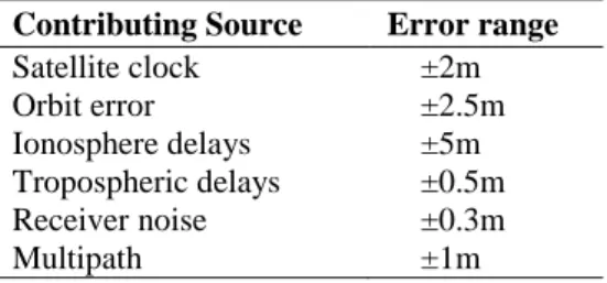
GNSS error sources and satellite geometry are the main factors that responsible for location accuracy of the required position. The main GNSS error sources are shown in the Table 3.1 (Jeffrey, 2015):
Table 3.1. GNSS error sources
3.1.1. Satellite Clocks
The atomic clocks drifts in the GNSS satellites with a small amount, in the same time they are very accurate. Unfortunately, a tiny imprecision in the satellite clock causes a big inaccuracy in the position which is calculated by the receiver. The GNSS ground control system monitors and compares the clock on the satellite to the even more accurate clock which is used in the ground control system. In the downlink data, the satellite supplies the user with an estimate of its clock offset. Typically, although the accuracy is able to make differentiate between different GNSS systems, the estimate has an accuracy of about 2 m. The GNSS receiver needs to recompense for the clock error to get higher position accuracy. Downloading precise satellite clock information from a SBAS or PPP service provider is a way to compensate for clock error. The precise satellite clock information includes corrections for the clock errors that were calculated by the SBAS or PPP system. Another way to compensate for clock error is to use a Differential GNSS or RTK receiver configuration. Later differential GNSS and RTK will be explained in detail (Jeffrey, 2015; Teunissen and Montenbruck, 2017).
3.1.2. Orbit Errors
GNSS satellites revolve around accurate and extremely distinguished orbits. However, when the satellite clock drifts by small variation in the orbit, it causes a great error to the calculated position. GNSS ground controlling system constantly monitors the satellites orbit. These ground control systems constantly send corrections to the satellites whenever there are changes in the satellites’ orbits. Therefore, the satellite ephemeris gets updated. There are small errors that still exist in the orbit resulting in up to around 2.5 m of the position error irrespective of the fact that ground systems constantly send corrections. Satellite orbit error can be minimizing in two ways. First, it is by downloading precise ephemeris information from a PPP service provider or an SBAS system. Secondly, it is using a RTK or Differential GNSS receiver configuration. Detailed
Contributing Source Error range
Satellite clock ±2m Orbit error ±2.5m Ionosphere delays ±5m Tropospheric delays ±0.5m Receiver noise ±0.3m Multipath ±1m
information on RTK, Differential GNSS and static will be discussed later (Jeffrey, 2015; Teunissen and Montenbruck, 2017).
3.1.3. Ionospheric Delay
The Ionosphere lies between 80 and 600 kilometres above the earth. This layer comprises of electrically charged particles that form ions. These ions pose a problem of delaying signals from the satellite thus resulting in a satellite position error of averagely 5 m, but these errors can increase especially when ionospheric activity is high. Ionospheric delay is not the same as solar activity time of season, year, location and day. Therefore, it is very difficult to predict the extent to which ionospheric delay impacts the calculated position. Also, radio frequencies of signals that pass through the ionosphere directly affect the ionospheric delay. For instance, GNSS receivers that receive more than one signal (L1 and L2) can exploit this attribute to their advantage.
The receiver can determine and remove this ionospheric delay from the position calculated. This is achieved by comparing L1 measurements to that of L2. For those receivers that can track only one GNSS frequency, ionospheric models are often used to reduce ionospheric delay errors. Unlike the use of various frequencies, models are not more effective at eliminating ionospheric delay. This is due to the changeable nature exhibited by ionospheric delay. In fact, ionospheric conditions are similar within any local area, and the rover receivers and base stations experience equal delays. This permits RTK systems and DGNSS to compensate any ionospheric delays. Ionospheric and tropospheric delay represented in Figure 3.2 (Jeffrey, 2015; Teunissen and Montenbruck, 2017).
3.1.4. Tropospheric Delay
The troposphere is the layer of atmosphere closest to the surface of the Earth. The changing humidity, temperature and atmospheric pressure in the troposphere can cause dissimilarities in tropospheric delay. Since tropospheric conditions are so alike within a local area, the base station and rover receivers experience almost the same tropospheric delay which allows DGNSS and RTK systems to recompense for tropospheric delay. To predict the amount of error caused by tropospheric delay, tropospheric models are used by GNSS receivers. Figure 3.2 shows the ionospheric and tropospheric delay (Jeffrey, 2015; Teunissen and Montenbruck, 2017):
Figure 3.2. Ionospheric and tropospheric delay
3.1.5. Receiver Noise
The position error that caused by the GNSS receiver hardware and software are referred by receiver noise. High end GNSS receivers are likely to have less receiver noise than lower cost GNSS receivers.
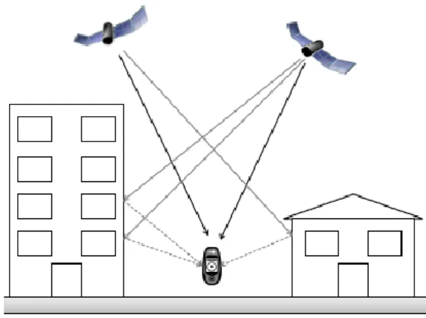
3.1.6. Multipath
The time of occurring multipath is when an object, such as the wall of a building reflects a GNSS signal to the GNSS antenna (Figure 3.3). As the reflected signal moves farther to arrive at the antenna, the reflected signal reaches the receiver a little late which can cause the receiver to estimate an inaccurate position. Placing a GNSS antenna in a location that is not close to the reflective surface is the simplest way to decrease multipath errors. The time that this process is not possible, the multipath signals must be dealt by GNSS receiver and antenna. The GNSS receiver typically handles the long delay multipath errors while short delay multipath errors are handled by the GNSS antenna. Due to the additional technology required to deal with multipath signals, high end GNSS receivers and antennas are likely better at rejecting multipath errors (Jeffrey, 2015; Teunissen and Montenbruck, 2017). Generally multipath can make an error in position of about (1—100) m or even more, depending on the multipath geometry.
Figure 3.3. Multipath error
3.2. Satellite Geometry
Satellites geometry is one of the major factors that affect the accuracy of a location. Often, when satellites sited close to one another, there are high chances that their signals will overlap thus reducing location accuracy. The broader the area of signal overlap, the larger the area of uncertainty. Figure 3.4 illustrates the three cases: The first, shows that the satellites are close to one another, this promotes poor GDOP. The second illustration shows a case where the satellites are located far from one another, and in this case good GDOP is experienced. In the third case, the satellites sited very far from each other, this results to good GDOP with a bad visibility. The effect caused by satellites geometry is often denoted by GDOP factor. The DOP is basically the ratio of positioning accuracy to that of the measurement accuracy. The DOP is greater than a unit, but if a number of satellites are observed (not less than 8) then value of DOP becomes less than unit. Depending on the factors that are utilized to calculate the DOP values, various variants are distinguished:
GDOP: overall accuracy; 3D-coordinates and time. PDOP: position accuracy; 3D-coordinates.
HDOP: horizontal accuracy; 2D-coordinates. VDOP: vertical accuracy; height.
TDOP: time accuracy; time in the case of GPS point positioning, which requires the estimation of 3-D position and receiver clock error, the most appropriate DOP factor is GDOP (Dawoud, 2012; Teunissen and Montenbruck, 2017).
Figure 3.4. Dilution of precision
3.3. Resolving Errors
Many techniques are available for resolving errors and obtaining required accuracy, the popular techniques are RTK, and static methods.
3.3.1. Static Method
Static GNSS survey procedures significantly assist in solving a number of systematic errors whenever high accuracy positioning is essential. The rationale of using Static GNSS procedures involves the need to make baselines among stationary GNSS units. This can be achieved by recording data continuously for a long period of time with respect to changes in the satellite geometry. This technique utilizes the constant data logs generated by various receivers at each point for a pre-planned period of time (Mwangi, 2009; Anonymous8, 2011; Anonymous4, 2012).
3.3.1.1. Methodology
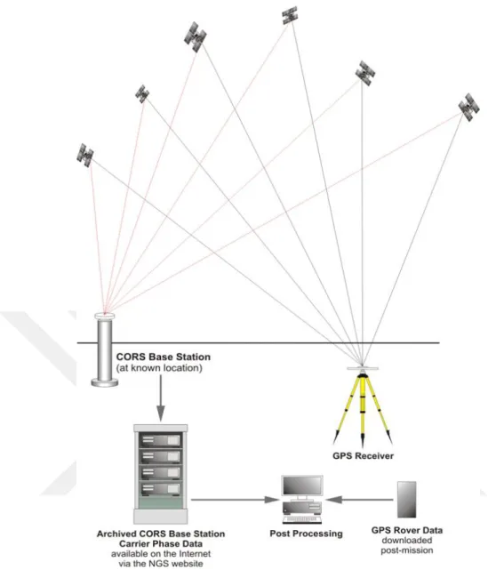
Pairs of GNSS receivers are set up in both known and unknown position stations. In most cases, one of the GNSS receivers is positioned over a location whose coordinates are well known (have been carried forward as on a traverse). The second receiver can also be positioned over a location whose specific coordinates are unknown. This technique desires to know the coordinates of the second receiver. Depending on the precision and conditions of observation required, it is mandatory for the two GNSS receivers to receive signals from the four or more similar satellites for a specific length of time. This period ranges from a few minutes to many hours. CORS stations are mostly regarded as the best base station since they are able to continuously make observations (Mwangi, 2009; Anonymous8, 2011), but in cases where the CORS stations are completely unavailable,
a specific point will make a suitable base station (Figure 3.5). The static method using CORS station shown in Figure 3.6.
During the observation window, all stations considered for survey are required to have a clear view of the sky, of not less than 15° above the horizon. An observation window represents a period of time during which the sky has all the observable satellites, thus allowing a successful survey to be carried out (Anonymous8, 2011).
On completion of the observation session, the GNSS signals received from both receivers undergo computer processing in order to determine the 3-Dimensional baseline vector components linking the points under observation. Both geodetic and local coordinates can be computed or adjusted using the vector distances (Anonymous8, 2011).
3.3.2. Fast-Static
Static GNSS surveys and Fast-Static GNSS surveys are the same except that their observation periods are shorter (approximately five to ten minutes). Unlike static GNSS method, Fast-static GNSS survey requires data reduction techniques and advanced equipment procedures. Anonymous6 (2000) points out that fast-static GNSS surveys should not be applied for surveys that require a horizontal accuracy which is greater than first order.
3.3.3. Times and Baseline Lengths
As accuracy and observation time are the main functions of a baseline length. Therefore, it is recommended to keep to a minimum all baseline lengths. Depending on the number of points and the area to be assessed by GNSS, it is advisable to consider setting up one or more reference stations. Radiating baselines from the temporary reference station spreads to several kilometres away. However, it is significant to reduce baseline lengths (Anonymous6, 2000).
In terms of accuracy and productivity, measuring short baselines (example 5 km) from various temporary references is more advantageous compared to measuring long baselines (example 15 km) from a specific central point.
Baseline Lengths Observation and Times are dependent on: Number of satellites
Ionosphere Baseline length Satellite geometry
Disturbance of ionospheric varies with day/night, time, year, month and earth's surface position at that particular period.
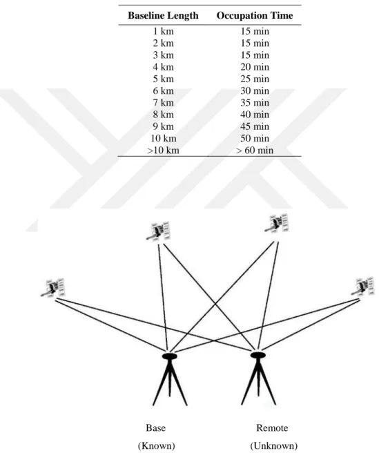
According to (Anonymous12) a good rule of thumb is 5 minutes per kilometer of baseline length with a minimum of 15 minutes. Table 3.2 shows a guide to observation times and baseline lengths.
Table 3.2. Relation between baseline length and approximate time observation required
Base Remote (Known) (Unknown)
Figure 3.5. Static method using a known point as a base station Baseline Length Occupation Time
1 km 15 min 2 km 15 min 3 km 15 min 4 km 20 min 5 km 25 min 6 km 30 min 7 km 35 min 8 km 40 min 9 km 45 min 10 km 50 min >10 km > 60 min
Figure 3.6. Static method using CORS base station (Anonymous3, 2017)
3.4. Kinematic GPS Surveys
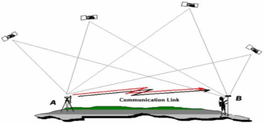
According to Mwangi (2009) and Anonymous8 (2011) RTK is a stop-and-go methodology that coordinates points which are accessible in real time. In RTK, a radio link is upheld between the rover and the base receiver. In this case, the base receiver provides the rover with pseudo-range, as well as carrier phase measurements that calculates its position and shows the coordinates which are updated regularly by the rover as it moves provided the satellites’ lock is maintained as shown in Figure 3.7.
3.4.1. Methodology
Basically two or more GNSS units are used for Kinematic GNSS surveys. At least one GNSS unit is installed and fixed over a known (reference) station. The other (rover)
GNSS units can shift from station to station. The entire baselines are produced from the GNSS unit which is occupying a reference station to the rover units. Kinematic GNSS surveys are consisted into two groups which are either continuous or “stop and go”. The duration of stop and go station observation periods are short, which is about two minutes. Dual-frequency LI and L2 GNSS observations techniques which are able to handle loss of satellite lock are used by RTK surveying (Anonymous8, 2011; Anonymous4, 2012).
The RTK technology allows the rover receiver so that the number of ambiguities can be started and resolved without a period of static initialization. With RTK, initialization can take place while it’s in a movement process if satellite lock happens to loss. Depending on the distance from the base station, the integers can be resolved at the rover in a period of 5—10 seconds (Anonymous8, 2011).
3.4.2. RTK Survey Procedure and Its Accuracy
Dual frequency LI and L2 GNSS receivers are essential to RTK surveying. The GNSS receivers are free to move from point to point except one of them which are installed over a known point. A radio connection and a processor or data collector are required when performing the survey in real time. The radio link is used to transport the raw data from the reference station to the rover (Anonymous8, 2011). In RTK the Achievable accuracies typically equal or exceed 10 mm (Manual, 2003).
Distances between the reference receiver and the rover are quite short which is ideally less than 3 km. Baselines above 5 km should be avoided if possible. And satellite geometry should be strong it means minimum 5 satellites should be available if possible 6 or more satellites (Anonymous5, 1999).
4. GPS (GLOBAL POSITIONING SYSTEM)
The first GNSS system was GPS. 1978s the American launched the first GPS (or NAVSTAR, as it is officially called) satellites for the US Department of Defense, and after that several generations (referred to as “Blocks”) of GPS satellites have been launched. At first, GPS was not available for civilian use; it was only available for military use, after that in 1983 it was decided to extend it to civilian use as well (Leick et al, 2015). A GPS satellite is shown in Figure 4.1.
Figure 4.1. GPS satellite
4.1. Space Segment
The time taken by each satellite to complete a full orbit is approximately 12 hours. Therefore, every GPS receiver is supplied with a minimum of 6 satellites in an open-sky from anywhere on Earth. Table 4.1 summarizes the Global Positioning System space segment. The satellites have been spaced in orbits so as to ensure the receiver view has a minimum of 6 satellites at any given point of time. The GPS satellites often broadcast their ranging signals, identification, satellite status and orbit parameters (corrected ephemerides).
The satellites can be recognized in two ways, either by their SVN or their PRN code. The GPS system space segment as a standard configuration includes 24 active satellites placed in MEO. The distance between the satellites and Earth is 20.200 km. The
US Air force has now lunched 27 operational GPS satellites in space plus 3 to 4 inactive satellites that can be reactivated when it is required. Each satellite transmits radio signals that travel at the speed of light to broadcast the navigation massages (Wiederholt and Kaplan, 1996; Leick et al, 2015; Anonymous2, 2017; Teunissen and Montenbruck, 2017).
Table 4.1. GPS space segment
In June 2011, the constellation has been overpopulated with up to 31 operational satellites. The first 3 satellites beyond 24 are placed into expandable slots within the baseline 24-satellite constellation. Each of the three slots B1, D2, and F2 may be split into two slots to accommodate up to 27 total satellites in the constellation (Table 4.2). Surplus satellites (operational satellites beyond the 27th) are typically placed in locations adjacent to satellites that are expected to require replacement the soonest (Teunissen and Montenbruck, 2017).
Affairs (2011) states that the constellation of GPS involves twenty-four operational slots located in the 6 equally-spaced orbital planes that surround the planet. Slot/plane scheme and the super positioning of satellite helps in making sure that the GPS users get the most precise navigation data whenever they want and at any place across the globe.
The 6 satellites in the existing GPS constellation were repositioned following a directed initiative by Expandable 24 (United States Strategic Command commander) and implemented by 2 SOPS. Based on the number of satellites and strength of the contemporary constellation, the revolutionary strategy was specially enacted by Air Force Space Command in order to benefit all the users in the planet. The ability of AFSPC to carry out this task was aimed at increasing the sturdiness of availability of satellite as well as the overall space signal performance through the expansion of three baseline twenty-four constellation slots (Affairs, 2011).
Table 4.2. GPS expandable slot designations (Anonymous9, 2017)
B D F
B5=B1F D5=D2F F5=F2F
B1=B1A D2=D2A F2=F2A
27 Plus 4 Spare Satellites 6 Orbital plans 55 degrees Orbital Inclination 20,200 km Orbit Radius
Anonymous2 (2017) report indicates that there were 31 operational satellites in GPS constellation as of 17th October 2017.
4.2. Control Segment
The Global Positioning System control segment comprises of one master control station, monitor stations, remote tracking stations and ground antennas as illustrated in Figure 4.2. There are sixteen monitor stations located across the world. Out of these, 6 are from the United States Air Force while 10 are from NGA.
Transmit signals from monitor stations are used to track the satellites. Monitor stations contain clock data, ranging signals, satellite ephemeris data, as well as almanac data. The master control station is served with the signals for recalculation of ephemerides after which the data uploading stations are used to transmit back the calculated ephemerides. Using the ground antennas located next to monitor stations, the Master Control Station controls and communicates with GPS satellites. AFSCN provides the master control station with additional information through remote tracking stations so as to improve tracking, telemetry and control. The control segment comprises of a group of monitoring stations which monitors, tracks, and maintains satellites. The master control station that is positioned in Colorado obtains data from all the monitoring stations then distributes them across the globe. It is also upon the monitoring stations to determine which information to be uploaded and which ground station to broadcast the control data straight to the respective satellites (Jeffrey, 2015; Teunissen and Montenbruck, 2017):
4.3. GPS Signals
Signals are received by the user segment at frequencies of L1 = 1575:42 M Hz, and L2 = 1227:60 MHz. The two carriers (L1 and L2) were selected so as to ensure that the signal is maximally strong against the effects of the ionosphere as well as weather conditions. These signals are produced in multiples of critical satellite clock frequencies i.e. fo= 10:23 MHz. L1 and L2 signals that have already been fed with processed data on their positions and their clock times from various satellites are received by the user. The American military and civilians are free to access L1. However, L2 can only be accessed by the military and US government since it carries signals that have been encrypted. These encrypted signals can only be decrypted by receivers belonging to the US government and their military. The carrier signals have 2 types of codes. One of the codes is known as Coarse Acquisition abbreviated as C/A while the other one is known as precise code abbreviated as P.
The L1 carrier is modulated with the C/A code and can be transmitted at 1:023 chips. The transmission of the code sequence is repeated after every 1 millisecond with an essential bandwidth of 1 MHz. This rate of chipping implies that one chip is 300 m long while the whole C/A code replicates itself after every 300 km during transmission. The Coarse Acquisition code encompasses information about time in relation to the satellite atomic clock during transmission of the signal. However, different satellites have different Coarse Acquisition codes and contain information about time in relation to the satellite atomic clock during the transmission of codes for their unique identification.
On the other hand, both L1 and L2 carriers are modulated with the P code. The difference between C/A and P codes is that P has the highest level of accuracy than the other. Precise code consists of approximately 1014 chips thus making it very long. This type of code is capable of getting transmitted by both L1 and L2 carriers at a chip rate of about 10.23 MHz meaning that P code’s resolution is ten times more than that of the C/A code. The P code sequence is repeated in every 38 weeks (Eissfeller et al, 2007; Leick et al, 2015; Teunissen and Montenbruck, 2017). GPS signal characteristics are shown in Table 4.3.
Table 4.3. GPS signal characteristics
4.4. GPS Modernization
Global Positioning System reached a fully operational capability in the year 1995 but a project was instigated in the year 2000 in an attempt to modernize the ground segments and Global Positioning System space. This would help in making use of new technologies, as well as user requirements. Creation of new signals and improvement of satellite signal strength and atomic clock accuracy are part of Space segment modernization. Moreover, modernization of the space segment includes addition of monitoring stations, improvement of in-orbit accuracy, as well as modelling the troposphere and ionosphere. As a result, the user equipment has realistically developed. Here the modernized signals are explained shortly (Jeffrey, 2015; Teunissen and Montenbruck, 2017):
L2C: The modernized Global Positioning System satellites broadcasts the designated L2C (a civilian signal) in order to ensure that the two civilian codes are accessible. The user can easily segment L2C for purposes of tracking it as it accurately delivers better navigation. Furthermore, L2C capable of directly measuring and removing ionosphere delay errors in a particular satellite by use of civilian signals in L1 and L2. It has been projected that 24 satellites will contain L2C signal by 2018.
L5: L5 is the 3rd civil Global Positioning System frequency that has already been
implemented by the United States at 1176.45 MHz. The GPS frequency is also
Designation Frequency Description
L1 1575.42 MHz
L1 is a modulated by the C/A code
(Coarse/Acquisition) which is available for all users and the P code precision which is encrypted for military and other authorized users.
L2 1227.60 MHz
L2 is a modulated by a P-code and, beginning with the block IIR-M Satellites and (L2C) civilian code. L2C has begun broadcasting civil navigation CNAV messages and discussed in (GPS modernization).
L5 1176.45 MHz
L5, available beginning with block IIF satellites, has begun broadcasting CNAV messages. The L5 signal is discussed in (GPS Modernization)
transmitted by modernized GPS satellites (higher than Block II-F). The frequency is beneficial in a number of ways including the ability to meet critical safety-of-life application requirements. Other benefits include provision of:
a. Signal redundancy
b. Better ionospheric correction c. Improved interference rejection d. Improved accuracy of signals
the L5 signal is anticipated to be transmitted from 24 satellites by the year 2021.
L1C: L1C has been designed to be the 4th civilian Global Positioning System
signal in the GPS satellites’ next generation (Block III). In its operational effect, L1C will be backwardly compatible with L1. It will also be greatly interoperable with Galileo. Additionally, the Indian IRNSS, Japanese QZSS, and Chinese BeiDou are planning to make L1C a paradigm for international interoperability as well as broadcast it. Implementation of L1C is seen as a new modulation scheme to make better the reception of GPS in major cities among other challenging environments. the 1st Block III satellites had been projected to be launched in 2016
5. GLONASS (GLOBAL NAVIGATION SATELLITE SYSTEM)
During the 1970s, the Soviet Union developed GLONASS as an experimental military communications system. After the end of the cold war, GLONASS was recognized by the Soviet Union to have commercial applications, through the system’s ability to transmit weather broadcasts, communications, navigation and reconnaissance data. The first GLONASS satellite was launched in 1982, and in 1993 it was declared that the system was fully operational. After declining the performance of GLONASS for a period of time, Russia committed to develop the system to the required minimum of 18 active satellites.
Now, GLONASS has a full deployment of 24 satellites in the constellation. GLONASS satellites have developed since the first ones were launched (Kleusberg, 1990; Langley, 1997; Teunissen and Montenbruck, 2017). The latest generation, GLONASS-M being readied for launch (Figure 5.1).
Figure 5.1. GLONASS-M satellite in final manufacturing
5.1. Space Segment
GLONASS Space Segment is made up of 24 satellites found in three orbital planes. Out of the 24, 21 are active while the rest are used as spares. This constellation confirms that the number of satellites available for broadcasting at any corner of the earth does not drop below 5. Dawoud (2012) says that a constellation of 21 satellites provides a simultaneous and continuous visibility of not less than 4 satellites over 97 percent of
the earth’s surface. He adds that a constellation of 24 satellites gives a simultaneous and continuous visibility of no less than 5 satellites over 99 percent of the earth’s surface.
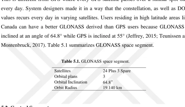
There are 24 satellites in a complete operational GLONASS constellation. The satellites are positioned in 3 orbital planes with an orbital radius of 19.140 km with 11 hours and 15 minutes’ orbital period. The main characteristic of a GLONASS constellation is that a given satellite passes over a similar earth’s spot after every 8 days. This is different from GPS where every GPS satellite passes over a similar spot once every day. System designers made it in a way that the constellation, as well as DOP-values recurs every day in varying satellites. Users residing in high latitude areas like Canada can have a better GLONASS derived than GPS users because GLONASS is inclined at an angle of 64.8° while GPS is inclined at 55° (Jeffrey, 2015; Teunissen and Montenbruck, 2017). Table 5.1 summarizes GLONASS space segment.
Table 5.1. GLONASS space segment.
5.2. Control Segment
System control centre is part of the Control Segment. The centre is situated in Krasnoznamensk Space Centre, about 40 km to the Southwest of Moscow. There are eight tracking stations that are connected and spread across Russia. The tracking stations monitor and track the status of satellites in the orbits. They also determine satellite clock offsets and ephemerides in relation to GLONASS time. Lastly, the stations use radio link to share the information with system control centre once every hour (Teunissen and Montenbruck, 2017).
5.3. GLONASS Signals
Similar codes can be transmitted by GLONASS satellites at varying frequencies. This kind of technique is referred to as FDMA. It is important to note that this technique is not the same as the one used by GPS. However, GLONASS and GPS signals have similar polarization (electromagnetic waves orientation), and signal power. The GLONASS system is anchored in 24 satellites with 12 frequencies which can be shared by transmitting the same frequency through antipodal satellites since the receivers on the
24 Plus 3 Spare Satellites 3 Orbital plans 64.8° Orbital Inclination 19.140 km Orbit Radius
ground show different times (Jeffrey, 2015). The satellites are positioned in an equal orbital plane separated by 180° as illustrated in Figure 5.2.
High and standard accuracy signals are provided by GLONASS, signals with high accuracy (modulated by P code on L1 and L2) are used by the military while the standard accuracy signals (modulated by C/A code on L1) are used by the civilians. The P code signal has no encryption. Table 5.2 shows the summarized GLONASS signals. Illegal use for P code is not recommended by the Russian Defence Ministry because it can easily be changed even without notice. February 2011 marked the successful launch of the new generation GLONASS-K satellite. Apart from L1 and L2 carriers, L3 carrier can be used by satellites to transmit signals in a frequency of 1204:704 MHz thus increasing accuracy and reliability where developers said that it may be used for life safety applications (Dawoud, 2012; Teunissen and Montenbruck, 2017).
Table 5.2. GLONASS signal characteristics
Figure 5.2. GLONASS antipodal satellites Designation Frequency Description
L1 1598.0625-
1609.3125 MHz
L1 is a modulated by the HP (High precision) and the SP (Standard precision) signals.
L2 1242.9375-
1251.6875 MHz
L2 is a modulated by the HP and SP signals. The SP code is identical to the transmitted on L1.
Both satellites are transmitting on the same frequency
5.4. GLONASS Modernization
When the service life of the current GLONASS-M satellites ends, they will be replaced with next generation GLONASS-K satellites that will provide the GLONASS system with new GNSS signals (Jeffrey, 2015; Teunissen and Montenbruck, 2017):
L3: A new civil signal designated L3 which is centered at 1202.025 MHz will be transmitted by the first block of GLONASS-K satellites (GLONASS-K1). L3, unlike the existing GLONASS signals, is based on CDMA which will make interoperability easy with GPS and Galileo. The first GLONASS-K1 satellite was launched in February 2011.
L1 and L2 CDMA: Two more CDMA based signals broadcast at the L1 and L2 frequencies are added by the second block of GLONASS-K satellites (GLONASS-K2). The FDMA L1 and L2 signals which are exiting now will be maintained transmitting and supporting legacy receivers. The first launch of GLONASS-K2 satellites was in 2016, A complete update of the full orbiting constellation will conclude in 2021.
L5: The third block of GLONASS-K satellites (GLONASS-KM) will add an L5 signal to the GLONASS system.
6. COMPARISON BETWEEN GPS AND GLONASS
Although GPS is more common as it provides higher accuracy signals compare to the other two in a wide range of the world, but for some reasons the Russian GLONASS system seems to operate more efficiently at northern latitudes as the purpose of GLONASS was to operate in Russia, home to some of the highest latitudes on the planet (Anonymous1, 2017).
The way of communication with receivers is believed to be the biggest difference between GPS and GLONASS. With GPS, the same radio frequencies are used by satellites but have different codes for communication. With GLONASS, satellites have the same codes but use unique frequencies. This allows satellites to communicate with one another despite being in the same orbital plane, while this is not a big problem with GPS. GPS and GLONASS are different in coordinate and time systems, it means the computed receiver position with GPS satellites is referenced to the coordinate system WGS84, and the computed receiver time is referenced to UTC (USNO). With GLONASS satellites alone the computed receiver position is referenced to SGS85, and the receiver time is UTC (SU) (Kleusberg, 1990; Bolduc, 2015).
GLONASS had reached its aim by the end of 2011, it had met the accuracy level in the absolute best environment (no cloud coverage, tall buildings or radio interference), to 2.8 meters. Although it made it a little less accurate than GPS, but for most military and commercial use cases it was completely acceptable (Bolduc, 2015).
6.1. Constellation Comparison between GPS and GLONASS:
GPS satellite constellation has 27 satellites in 6 orbital planes inclined at an angle of 55°, relative to the equator. Additionally, there are three backup satellites in the constellation. Orbits are virtually spherical with less than 0.02 eccentricity and 26 560 km semi-major axis altitude of 20 200 km. At this height, orbits are called MEO. Satellites move at a speed of 3.9 km/second and approximately 12 hours’ nominal period with the geometry repeating each sidereal day. GPS space vehicles are arranged on six planes each containing a minimum of four slots. The current configuration enables users to simultaneously observe a minimum of four satellites in view globally, with a 15° masking angle of elevation (Anonymous10, 2017).
There are nominally 24 operational satellites in a standard GLONASS constellation and 3 satellites as a spare. The satellites are distributed across 3 orbital
planes with a difference of 120° longitudinal ascending node from one plane to the other. Each plane has 8 satellites separated in 45° argument of latitude. Moreover, 2 different orbital planes of satellites in equal slots have an argument of latitude difference of 15°. Every satellite has a unique slot number which is used to show its location in the plane and define the orbital plane (Anonymous11, 2017).
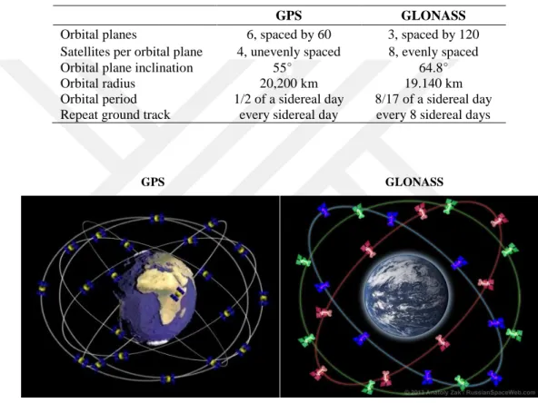
The difference between GPS and GLONASS orbitals shown in Table 6.1. And Figure 6.1 shows the orbits of GPS and GLONASS.
Table 6.1. Orbital comparison (Kleusberg, 1990)
GPS GLONASS
Figure 6.1. Orbital comparison
6.2. Comparison of signal characteristics between GPS and GLONASS
Signal characteristics have been explained before, here a brief comparison shown between GPS and GLONASS signals (Table 6.2.).
GPS GLONASS
Orbital planes 6, spaced by 60 3, spaced by 120
Satellites per orbital plane 4, unevenly spaced 8, evenly spaced
Orbital plane inclination 55° 64.8°
Orbital radius 20,200 km 19.140 km
Orbital period 1/2 of a sidereal day 8/17 of a sidereal day
Table 6.2. The nominal satellite signal characteristics (Kleusberg, 1990) GLONASS GPS L1: (1,602 + k × 9/16) MHz L2: (1,246 + k×7/17) MHz K=channel Number L1: 1,575.42 MHz L2: 1,227.60 MHz Carrier signals
Same for all satellites C/A code on L1 P-code on L1 and L2
Different for each satellite C/A-code on L1, P-code on L1 and L2 Codes C/A-code:0.511 MHz P-code: 5.11 MHz C/A-code: 1.023 MHz P-code: 10.23 MHz Code frequency
Clock and frequency offset Clock offset, frequency
Offset, frequency rate Clock data
Satellite position, velocity and acceleration every half hour Modified keplerian orbital
elements every hour Orbital data
6.3. Comparing GPS Only and GPS + GLONASS
Combining GPS and GLONASS means primarily the building of receiver that can simultaneously track GPS and GLONASS signals. Ranges measured on these signals must be combined with GPS and GLONASS clock and orbital data to compute the receiver’s position.
The most obvious advantage of a combined system is the availability of twice as many satellites of the total of 48 satellites, at least 12 will be visible anywhere at any time.
In land navigation, it’s not as high a priority as in civil aviation navigation, vehicles sometimes have to be navigated in some places under severe shadowing conditions, mostly in the cities and mountainous areas. In these cases, GPS or GLONASS alone cannot supply sufficient coverage for position solution. Studies have shown that a combined system will yield a robust navigation solution even if the satellite visibility is more or less completely blocked on one side of the sky.
The last predictable advantage in the survey is economical in nature. In order to find out the three-dimensional baseline vector between survey markers with centimeter accuracy, surveyors use GPS carrier phase measurements in a differential static mode of operation. This accuracy is available if measurements are accumulated over several tens of minutes. If the number of satellites is doubled through a joint system, a huge reduction of the essential measurement time may occur (Kleusberg, 1990).
In DGNSS, using GPS only if comparing with GPS + GLONASS for RTK and static methods, obtains a lower number of satellite availability, lower accuracy in
centimeters, lower position quality, and in obstructed areas also losing signals will be so common. But while performing RTK and static methods with DGNSS in GPS + GLONASS provided a better quality, accuracy, increasing satellite. In Numerical Application part, more details about the advantages and performance of combined GPS + GLONASS for RTK and static methods will be discussed, theoretically and numerically.
7. NUMERICAL APPLICATION
7.1. Test Description
For testing RTK and static GPS, RTK and static GPS + GLONASS a field work was performed in April 2017, in Erbil city of Iraq, which locates at lat. 36.191113 degree, long. 44.00916 degree. The study area is near Shanadar Park in the city center of Erbil. This area is selected because in spite of open sky, also obstructed sky were available because of trees and buildings(Figure 7.1 and Figure 7.2).
The Leica viva GS15 GNSS receiver was used, that it has 120 channels and this dual frequency receiver is capable of receiving GPS and GLONASS signals (Anonymous7, 2012). Some of the technical specifications of the Leica viva GNSS receiver are shown in Tables 7.1, 7.2, and 7.3.
In this project the reference point ER01, which is an official reference point in the country, used as a base station for both RTK and static. The point was established on WGS84 datum.
For RTK, 14 points were established and measured in the area (Figure 7.1 and Figure 7.3). Occupation times for each point was 5 seconds and simple rate or epoch was 1 second, and elevation cut-off angle was 15° for normal RTK process, WGS84 was used as a datum, and L1 and L2 signals were received. Each point measured two times; First, points were measured with GPS + GLONASS mode which the receiver will receive signals from GPS and GLONASS satellites together. Second, measuring the same points using GPS only mode that the receiver will only receive signals from GPS satellites.
In the same area, also a rapid static method was performed and 3 points (BM1, BM2, BM3) were established with GPS + GLONASS in open sky, 15 minutes’ observation accepted for each point, because of having short baselines of about 100 m. The relation between baseline length and approximate time observation was explained before. Then data processing started using Leica Geo office software for the RINEX data, which contains GPS + GLONASS signals. Later by using the Leica Geo Office software the GPS signals was exported from the combined RINEX, a new RINEX file made that contains GPS only signals. After data processing for the GPS only RINEX file also, the coordinates and standard deviations of points were obtained. Since the baseline is too small in rapid static, so observations will be in the same ionospheric condition. WGS84 used as a datum, after that the data is projected to UTM at zone 38 of north. Table 7.4 shows the selected processing parameters for post processing.
Tests under an obstructed sky were not performed for static, because in static method we are about establishing control points, which always requires the maximum accuracy possible, and always better satellite availability and more suitable locations will be more preferred. It doesn’t make sense to put control points under an obstructed area, in case if you have another choice, because when an accuracy with millimeters is requires, choosing the best location for receiving signals and satellite availability needs to be chosen first, and also points must be well located which provide a good visibility for the project. So in case of performing a test like static in obstructed area, the results will not be that useful for the users, because normally users should not put it under the closed sky.
Figure 7.1. Satellite images of working area (Erbil City, Iraq) Working Area
Figure 7.2. Working area.
Table 7.1. Satellite signal tracking (Anonymous7, 2012)
Table 7.2. Accuracy (rms) with RTK (Anonymous7, 2012)
Standard of compliance Compliance with ISO17123-8
Single Baseline (<30 km) Horizontal: 8 mm + 1 ppm (rms) Vertical: 15 mm + 1 ppm (rms)
Network RTK Horizontal: 8 mm + 0.5 ppm (rms) Vertical: 15 mm
+ 0.5 ppm (rms)
Table 7.3. Accuracy (rms) with post processing (Anonymous7, 2012) Static (phase) with long
observations
Horizontal: 3 mm + 0.1 ppm (rms) Vertical: 3.5 mm + 0.4 ppm (rms)
Static and rapid static (phase) Horizontal: 3 mm + 0.5 ppm (rms) Vertical: 5 mm + 0.5 ppm (rms)
Kinematic (phase) Horizontal: 8 mm + 1 ppm (rms) Vertical: 15 mm +
1 ppm (rms)
Obstructed Area Open Sky
Features GPS: L1, L2, L2C, L5 GLONASS: L1, L2
Galileo (Test): GIOVE-A, GIOVE-B Galileo: E1, E5a, E5b, Alt-BOC BeiDou: B1, B2
Table 7.4. Selected processing parameters for post processing
From the elements of the variance-covariance matrix of the horizontal coordinates and elevations of any point, standard deviations and position qualities of easting, northing, elevation, can be determined.
Variance-covariance matrix,
𝐶 = [
𝑄11 𝑄12 𝑄13
𝑄21 𝑄22 𝑄23
𝑄31 𝑄32 𝑄33] (1)
Standard deviation of easting,
𝜎𝐸= 𝑚0√𝑄11 (2)
Standard deviation of northing,
𝜎𝑁= 𝑚0√𝑄22 (3)
Standard deviation of elevation,
𝜎𝑧= 𝑚0√𝑄33 (4)
Position quality of coordinates, 𝜎𝑝 = √𝜎𝐸2+ 𝜎𝑁 2 + 𝜎𝑍 2
Parameters Selected
Cut-off angle: 15°
Ephemeris type: Precise
Solution type: Automatic
GNSS type: GPS + GLONASS
Frequency: L1 + L2
Fix ambiguities up to: 80 km
Min. duration for float solution (static): 5' 00"
Sampling rate: Use all
Tropospheric model: Hopfield
Ionospheric model: Automatic
Use stochastic modelling: Yes
Min. distance: 8 km
7.2. Test Results
The results show that for RTK method the position quality or accuracy was about 1 cm when using GPS + GLONASS, and near 1 cm better than using GPS only in unobstructed area, including points 1—10 (Figure 7.3). However, in obstructed area the position quality was about 2—3 cm for GPS + GLONASS and near 3 cm better than GPS only, as it can be notice from points 11—14 which locates in the obstructed area (Figure 7.3). The coordinate differences, standard deviations and position qualities of the points are shown in Tables 7.5, 7.6, and also see Figures 7.4, 7.5, 7.6, and 7.7.
Generally, in RTK method the combining system showed a better accuracy, better position quality and provided a better satellite availability. With cut of angle 15°, the maximum 8 satellites were available when using GPS only in unobstructed area, and in obstructed areas the satellite number for GPS only was about only 4—5 satellites, while more than 14 satellites were available when using GPS + GLONASS in unobstructed area and at least 8 satellites were available in obstructed area. Combined GPS + GLONASS reduced the chances of signal loss and multipath, and less observation time was required by providing a better satellite geometry because of increasing the number satellite availability.
Table 7.5. Coordinate differences between GPS + GLONASS and GPS only in RTK method [m]
Table 7.6. Standard deviations and position qualities of points in RTK method [m]
Figure 7.4. Standard deviations of easting in RTK method [m] 0 0.005 0.01 0.015 0.02 0.025 0.03 0.035 0.04 0.045 1 2 3 4 5 6 7 8 9 10 11 12 13 14 Stan d ar d Dev iatio n ( E asti n g ) Points GPS + GLONASS GPS only Points ∆X ∆Y ∆Z 1 0.0099 0.007 -0.0156 2 0.0036 0.004 -0.012 3 0.0013 0.006 -0.0185 4 0.0048 0.006 0.0034 5 0.0042 -0.001 -0.008 6 0.0043 0.001 -0.0047 7 -0.0006 0.004 -0.0072 8 0.0009 0.004 -0.0056 9 0.0024 0.006 0.0312 10 -0.0034 0.008 0.0393 11 -0.016 0.02 0.016 12 -0.043 0.01 0.029 13 -0.137 0.106 0.078 14 -0.011 -0.024 0.005 GPS + GLONASS GPS only Points 𝝈𝑬 𝝈𝑵 𝝈𝒁 P.Q 𝝈𝑬 𝝈𝑵 𝝈𝒁 P.Q 1 0.00568 0.00514 0.00765 0.0108 0.00661 0.00619 0.00821 0.0122 2 0.00637 0.00523 0.00845 0.0118 0.00712 0.00831 0.0124 0.0165 3 0.00581 0.00622 0.00819 0.0118 0.00716 0.00821 0.0128 0.0168 4 0.00562 0.00674 0.00793 0.0135 0.00842 0.00879 0.00983 0.0156 5 0.00495 0.00484 0.00846 0.0109 0.00814 0.00829 0.0112 0.0161 6 0.00539 0.00547 0.00734 0.0106 0.00842 0.00876 0.0131 0.0179 7 0.00653 0.00679 0.00967 0.0135 0.00751 0.00814 0.0143 0.0180 8 0.00586 0.00593 0.00869 0.0120 0.00803 0.00812 0.0152 0.0191 9 0.00541 0.00568 0.00828 0.0114 0.00915 0.00946 0.0123 0.0180 10 0.00684 0.00695 0.00978 0.0138 0.00821 0.00907 0.0131 0.0179 11 0.01324 0.01385 0.01623 0.0251 0.02046 0.01915 0.02413 0.0370 12 0.01638 0.01454 0.01751 0.0280 0.02358 0.02658 0.02974 0.0463 13 0.01127 0.01236 0.01623 0.0233 0.03943 0.03841 0.04982 0.0742 14 0.01473 0.01396 0.01659 0.0262 0.03297 0.03284 0.04023 0.0615
Figure 7.5. Standard deviations of northing in RTK method [m]
Figure 7.6. Standard deviations of elevation in RTK method [m]
Figure 7.7. Position qualities of points in RTK method [m] 0 0.005 0.01 0.015 0.02 0.025 0.03 0.035 0.04 0.045 1 2 3 4 5 6 7 8 9 10 11 12 13 14 Stan d ar d Dev iatio n ( No rth in g ) Points GPS + GLONASS GPS only 0 0.01 0.02 0.03 0.04 0.05 0.06 1 2 3 4 5 6 7 8 9 10 11 12 13 14 Stan d ar d Dev iatio n ( E lev atio n ) Points GPS + GLONASS GPS only 0 0.02 0.04 0.06 0.08 0.1 0.12 0.14 0.16 0.18 0.2 1 2 3 4 5 6 7 8 9 10 11 12 13 14 P osi ti on Q ual it y POINTS GPS + GLONASS GPS only