QA
7 · £ · 6 4 ·
DESIGN AND SOFTWARE IMPLEMENTATION OF
LIBRARY FUNCTIONS FOR ELECTRONIC
CIRCUIT SIMULATION
A THESIS
SUBMITTED TO THE DEPARTMENT OF ELECTRICAL AND ELECTRONICS ENGINEERING
AND THE INSTITUTE OF ENGINEERING AND SCIENCES OF BILKENT UNIVERSITY
IN PARTIAL FULFILLMENT OF THE REQUIREMENTS FOR THE DEGREE OF
MASTER OF SCIENCE
By
Mustafa Nazim Yazgan
1994
Θ,Α
6
(-f
‘ V 35
I certify that I have read this thesis and that in my opinion it is fully adequate, in scope and in quality, as a thesis for the degree of Master of Science.
ÂÂ q
\
aa/\
a iİ
îA ^
Assoc, rrof. Dr. M. Ali Tan (Sup^rvisor)
I certify that I have reeid this thesis and that in my opinion it is fully adequate, in scope and in quality, as a thesis for the degree o f M<ister of Science.
Prof. Dr. /Abdullah Atalar (Co-Supervisor)
I certify that I have read this thesis and that in my opinion it is fully adequate, in scope and in quality, as a thesis for the degree o f Master of Science.
Assoc. Prof. Dr. Omer Morgiil
I certify that I have retid this thesis and that in my opinion it is fully adequate.
Approved for the Institute of Engineering and Sciences:
A M
Y
Prof.^ Dr. Mehmet B a r a y ^
ABSTRACT
DESIGN AND SOFTWARE IMPLEMENTATION OF
LIBRARY FUNCTIONS FOR ELECTRONIC CIRCUIT
SIMULATION
Mustafa Nazim Yazgan
M.S. in Electrical and Electronics Engineering
Supervisor: Assoc. Prof. Dr. M. Ali Tan
Co-Supervisor: Prof. Dr. Abdullah Atalar
1994
In this thesis, the software implementation of “SIMLIB” , a library of elec tronic circuit simulation, is described. The building blocks of a circuit sim ulator, namely, input parser, types of analyses, methods and matrix solvers are discussed. The algorithms and some special techniques employed in this library, as well as ways of modifying the program are explained. SIMLIB has become a good environment for the researchers to try гınd develop new ideas on circuit simulation.
Keywords :
Computer-Aided Design, Electronic circuit simulation, SPICE, AWE, AC ainalysis, DC analysis, Transient analysis, Newton-Raphson itera tion, Trapezoidal approximation, Matrices, C-f-+ programming language.ÖZET
ELEKTRONİK DEVRE SİMÜLASYONU İÇİN YAZILIM
TASARIMI VE GERÇEKLENMESİ
Mustafa Nazım Yazgan
Elektrik ve Elektronik Mühendisliği Bölümü Yüksek Lisans
Tez Yöneticileri: Doç Dr. M. Ali Tan
Prof. Dr. AbdullaJı Atcdar
1994
Bu tezde, bilgisayar destekli tasarım yardııruylageliştirilen, “SIMLIB” adını verdiğimiz bir elektronik devre simûlasyon paketi anlatılmıştır. Öncelikle dev re simûlasyonunun temel parçaları olem girdi okunuşu, analiz türleri, metodlar ve matris çözücüler hakkında kısa bilgiler verilmiş, ardından hazırlanan bu pakette kullanılan algoritmalar, özel teknikler açıklanmıştır. Bu paket prog rama eklemelerin ve yeniliklerin nasıl yapılacağı belirtilmiştir. SIMLIB, devre simülasyonu ile ilgelenen ariiştımacıların yeni fikirlerini denemeleri ve uygula maları için oldukça faydalı bir ortam oluşturmuştur.
Anahtar kelimeler :
Bilgisayar destekli tasarım. Elektronik devre simülasyonu, SPICE, AWE, AC analiz, DC analiz. Geçici durum analizi, Newton-Raphson iterasyonu, Trapezoid yгıklaşım, Matrisler, C-f-f- program lama dili.ACKNOWLEDGEMENT
I would like to express my deepest gratitude to Dr. M. Ali Тал aлd Dr. Abdullah Atalar for their supervision, guidance, suggestions and encour agement throughout the development of this thesis.
I would like to thank Ogem Ocah for his collaboration and invaluable help on the implementation o f this work. I would also like to thank Satılmış Topçu aлd Mustafa Çelik, members o f the CAD group at Bilkent University, and all of my friends for their moral support.
TABLE OF CO N TEN TS
1 INTROD UCTION 1
2 BASIC CONCEPTS OF A SIM ULATOR 5
2.1 Input P arser... 5
2.2 Types o f Analyses... 7
2.3 Matrix S e t u p ... 15
2.3.1 Matrix Solvers... 18
3 ALGORITH M S AN D IMPLEM ENTATION 19 3.1 Algorithm of Input P a r s e r ... 19
3.2 Algorithms of A nalyses... 20
3.3 Algorithm o f AWE Method ... 22
3.4 Im plem entation... 26
3.5 M o d ific a tio n ... 27
3.5.1 Adding a New D e v i c e ... 27
3.5.2 Adding a New A n a ly s is ... 32
A SIMLIB M A N U A L 38 A .l E le m e n ts ... 38 A .2 AneJyses... 4Q A . 3 Output fo r m a t t in g ... 40 B DATABASE 41 B . l Global Declarations... 41 B.1.1 C ir c u it... 41 B.1.2 Devices ... 41 B.2 J o b s ... 43 B.3 S u b circu it... 44 B.4 M a tr ix ... 44 C STENCILS 45 D M A T R IX and TABLE PACKAGES 53 D .l Matrix pcickages... 53
D. 2 Table Package... 54
E LISTINGS 56 E . l Simiib Directory S tru ctu re... 56
E.2 Global variables and fu n ction s... 59
E.3 Two terminal device c l a s s e s ... 60
E.4 Four terminal device c la s s e s ... 64
E.5 Moment c l a s s ... 66
E. 7 MNA setup fu n ction s... 67
F EXAM PLES 68
F . l DC sweep analysis of a BJT in v e r t e r ... 68 F.2 AC analysis of a transmission line c ir c u it ... 70 F.3 Transient analysis o f a nonlinear dynamic circuit... 72
LIST OF FIGURES
2.1 Input Parser Flow C h tir t... 6
2.2 A Simple RC C ir c u i t ... 7
2.3 AC Equivalent of RC C ircuit... 8
2.4 C a p a c it o r ... 9
2.5 Norton equivalent o f a capacitor using Trapezoidal Approximation 10 2.6 Simple Diode C ir c u it ... 10
2.7 Linearization of D i o d e ... 11
2.8 Newton-Raphson Algorithm Flow D iagram ... 12
2.9 Diode M od el... 13 2.10 Nonlinear DC A n a ly sis... 13 2.11 DC Sweep A n a lysis... 14 2.12 AC A nalysis... 14 2.13 Transient Analysis ... 15 2.14 Stencil o f a Resistor... 17
3.1 Diagram of the Polynomial Root Finder ... 25
3.2 Flow diagram of Moment M a tch in g ... 25
3.3 Analysis vs. Elements ... 26
C .l A Transmission L i n e ... 49
C.2 A T w o - p o r t ... 51
F .l Three stage BJT inverter... 69
F.2 Output waveforms of the BJT in v e r t e r ... 70
F.3 Example circuit for AC an alysis... 71
F.4 Frequency response of the transmission line circu it... 71
F.5 Example circuit for tr<insient analysis... 72
Chapter 1
INTRODUCTION
In 1958, the fabrication of integrated circuits (IC’s) containing transistors and their interconnections on a single substrate was realized. The adv<tnces in IC technology are still continuing from that time on. By time, the capacity of IC’s has increased to contain millions of triinsistors on a very small area of silicon.
The fabrication process o f IC’s is гm expensive procedure. Therefore, the analysis of the designed IC before its implementation plays an import£uit role. If the an£ilysis step is not taken into «iccount, some fatal bugs and errors in the design stage will end up with a costly, but useless chip.
The traditional way of analyzing simple circuits is the hand calculation. However, the complexity of the integrated circuits has reached such a level that the hand calculation of the entire circuit is almost impossible. A detadled verification by hand calculations of even a small part o f a complex IC design takes an excessive amount o f time. An economic solution to this problem is computer-iiided analysis. At this step, the concept of “simulation” of electronic circuits on computers arises.
Circuit simulation provides veirious eidvantages. Circuit modifications and corrections can be made before implementation. Eliminating such errors in an early design stage may lead to considerable savings in design cost and time. The second important point is that, extensive simulation capabilities gives the designer a deeper insight into the circuit behavior.
The circuit simulation techniques introduced in 1950s were used to ana lyze circuits with tens of transistors. Today, even though basically the same
techniques are used, the capacity o f the simulators have increased to simu late circuits with tens of thousands of transistors. The advances in desktop workstations and parallel machines have forced researchers to adapt circuit simulators to the latest hardware developments. Nevertheless, accuracy and speed are two opposing f<ictors in circuit simulation. Therefore, the need for novel approaches and new methods continues.
An industry standtird for electronic circuit simulation is SPICE [1]. SPICE combines Modified Nodal Analysis (M NA) [2] with TVapezoidal Integration (in its time domain transient mode) and Newton-Raphson (NR) iteration [3], [4]. The combination of algorithms that forms the core o f SPICE has been in use, with minor modifications, since mid-1960s. There have been meuiy attempts to improve upon SPICE, but no simulator has managed to replace its industry standard status.
Need For New Circuit Simulators
Everyday, new ideas and new methods are introduced to analyze circuits and systems. Also, the technological developments force simulators to cover new devices and simulate larger circuits. The point is to make simulators work faster, more efficiently, ciccurately and adaptively.
Some of the new methods used in the griiduate studies at Bilkent University can be given as follows:
Asymptotic Waveform Evaluation (AW E) technique Wcis introduced by Lawrence Pillage and Ronald Rohrer from Ceirnegie Mellon University, [5] to analyze the transient response of RLC circuits, by matching the initial boimd- ary conditions and a number of moments o f the actual circuit to that o f a reduced order of poles. Some of the simulation studies in Bilkent have been based on this concept.
Piece-wise Linear Asymptotic Waveform Evaluation (PLAW E) is a simulator package that employs AWE method, and uses piece-wise linear models of non linear circuit elements. [6] The former implementation was realized by a group of graduate students at Bilkent University. That has been followed by a de tailed research on PLAWE by Satılmış Topçu, as a Ph.D. study at the same university [7].
Nonlinear AWE (NOW E) method is proposed by Ogan OcaJi, as a nonlinear version of AWE method, that covers tmalysis of circuits having nonlinear ele ments [8].
Generalized AWE (GAW E) is amother extension o f AWE method which uses multi point moment matching. This is the Ph.D. subject of Mustafa Çelik (9].
The method is especially employed for AC analysis of electronic circuit at high frequencies.
As it is seen that there has been a number of new studies on circuit simu lation at Bilkent University, which have to be investigated immediately to see whether they are worth studying or not. This is the point that has become the motivation of this work. Therefore, it is decided to implement a new circuit simulation tool.
The main goal is to create an eeisy-to-modify and extendible library which can be used to develop new circuit simulators. The program which is imple mented in this Master’s Thesis, consists a library of circuit analysis, that is called as
SIMLIB.
Furthermore, any type o f devices, analyses, methods can easily be abided to this library. The style o f programming is also a concept that has to be taken into account, so that further work on the program could be carried out easily.As the result o f this study, a complete set of library is implemented. A simulator based on these modules is written. The modules are, input parser, sparse matrix setup and solver, Newton-Raphson iteration, DC circuit solver, DC sweep aniJysis, AC analysis, transient analysis and some circuit element libraries, which will be explained in the following chapters.
The program is implemented in C-f-h [10] on Sim * * Workstations running under UNIX ^ operating system.
C -f-f is a version of C, a very common programming language. It is designed to
- be a better C
- support data abstraction
- support object-oriented programming (OOP).
The styles of programming typically used in C are “procedural programming” and “modular programming” . C-f-l- is a “better C” , because C -f-f provides better support for these styles o f programming than C does, while C+-|- does not lose any generality and efficiency and remciins almost completely a superset of C.
It is apparent that OOP will be the programming style of the future because of its advzmtages over most of the classical languages. Therefore, it has been decided to implement the libraries in C+-1-.
‘ SUN is a trademark o f Sun Microsystems. *UNIX is a trademark o f A T& T Bell Laboratories.
In Chapter 2, a brief discussion on some basic building blocks of a circuit simulator, that are implemented in SIMLIB is presented to explain what a circuit simulator does conceptually. Moreover, Chapter 3 leads the new pro grammers to the details o f the program. In this chapter, the implementations o f input parser, analyses and AWE method are shown in an algorithmic way. In the same chapter, the implemented parts o f SIMLIB axe listed and adding a new type o f analysis and a new element to this librau-y is given with an exam ple. This part o f the thesis, together with the appendices is prepared to serve as a manual for SIMLIB.
Chapter 2
BASIC CONCEPTS OF A
SIMULATOR
In this chapter, three basic parts o f an electronic circuit simulator are covered briefly. In the first section, the interpretation o f the circuit declaration (in other words Input Parser) is explained. In the second section, some types of гmalysis that are applied to electronic circuits are introduced. Some methods employed in these analyses are also mentioned. In the third section, formulation of the circuit in matrix form is discussed.
2.1
Input Parser
Generally, an electronic circuit is described in text format so that it can be viewed and typed by human beings. However, this style of declaration has to be interpreted by the simulation progrcim to carry out the operations faster and easily using its internal database, this jo b is done by the
parser
. Furthermore, the input parser has to make error detection and correction to prevent from the erroneous results, and warn the user for wrong declarations.Inputs and Outputs
The input that is eiccepted by SIMLIB is a SPICEl-like circuit definition as a text file. The style of the definitions are explained in Appendix A, SIMLIB Manual. The output is the global variable “circuits” , which is an interntJ struc ture consisting the circuit definition, devices, models, anedyses to be performed,
output formats, etc. (see Appendix B)
Two main functions of the input parser are:
First Pass Counts the number o f each device, puts the node names in the node table, puts the voltage source names (or current-controlled elements) in the voltage source table (table structure is explained in Appendix D), checks the number of parameters of the device declarations and reports errors.
Second Pass Converts the node names and voltage source names into index numbers using the tables, checks the parameters, initirdizes the values of some devices. The index numbers will be used as pointers to the elements of matrix that will be formed during the analysis parts.
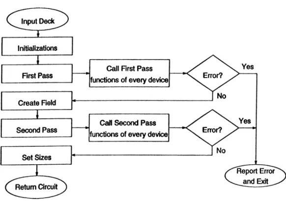
The program flow chart o f the input parser is shown in Fig. 2.1.
Figure 2.1: Input Parser Flow Chart
M od u la rity o f the in p u t parser
Every device is responsible for checking errors and setting up its field in the memory. Therefore, if addition of a new device or a new type of option card is required, its new first pass, second pass, and field creation functions should be created. Adding a new device and type of anaJysis aure explained in Chapter 3, Section 5 in detail.
E rrors h an dled
Undefined cards and devices are reported. Specific input errors belonging to a device are htindled in its corresponding functions, such as, unexpected number of pzu-ameters and typing errors of numbers.
2.2
Types of Analyses
The main part of a simulator is the analysis part. The operations that will be performed on the circuit is defined in this ptirt. There are a number of ainalysis types that are mainly applied to electronic circuits. Also, the new methods have been introduced in some of these aneilyses. However, since the aim in this work is not to cover all the existing analyses and methods, it is tried to build an extendible library, which can be used to develop any kind o f analyses. Nevertheless, most common ones cure implemented. They are considered in this section.
The types o f analyses are explained in brief, on the following simple exam ple. The manual method is employed for this section.
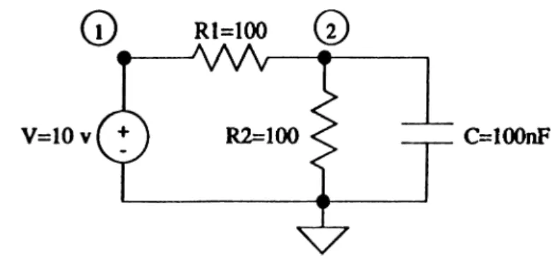
DC Analysis
C=100nF
Figure 2.2: A Simple RC Circuit
The circuit in Fig. 2.2 consists only two resistors, a capeicitor and a voltage source. Therefore, it is a linear, dynamic circuit. First of all, consider the DC operating point. The capaicitor can be discarded in this case and writing down the KCL and KVL equations, the unknowns — current through the voltage source, and the node voltages— are found as follows:
tV - *m = 0
Vr i = Cl — cj = İr \ · jRl ^R2
=
= XR2· B2
tV = 50mA, Cl = lOV, cj =
bV
This is the DC operating point solution of the linear circuit.
A C Analysis
AC analysis can also be called as the frequency response o f the circuit. This time, the capacitor is replaced by a frequency dependent complex valued resistor. And the value of the voltage source is replaced by 1 (that is, the magnitude). The equivalent circuit is shown in Fig. 2.3. At this step, the same type of operations as in the DC anaJysis part will be carried out on the given range of frequencies. These operations are complex due to the value of the capacitor-and in general, dynamic elements. Then the AC analysis of the circuit is completed.
j(oC
Transient Analysis
In this type of amalysis, the response o f the circuit is examined as the function of time. In this case, the dynamic elements, energy storage elements have to be taken into account. This analysis is generally used to compute the delay o f the circuits, and how they respond to different inputs (impulse, step, ramp, pulse).
The transient behavior of the above example is calculated exactly as follows (initial voltage on capax:itor is assumed to be zero):
Vc{t) = Vv
R2
Ri
+Ri
where
Vy
is the value of the voltage source.-However, the solution is not that easy for larger circuits. The exact solution can not be formulated in most o f the cases. Then, some approximations, which are used to linearize the circuit, have to be done. In this work, the trapezoidcil approximation is used.
TVapezoidal Approximation
In the transient analysis o f the dynamic devices, like capacitors and induc tors, integration approximations have to be used to express them as a set o f linear equations.
Consider a capacitor as an example: O + ·
i = C
T
dv
dt
Figure 2.4: CapacitorThe capacitor voltage in terms of the integral of the capacitor current is:
1
1
v{t + Ai) = v(t) -I- - jf
t(r)d-One can consider approximating the integral equation in three possible ways:
f(t+^0
jf
t(r)dr
At · t(i)
At · i(t + At)
Forwau-d Euler (FE) Backward Euler (BE) 2 [*(0 + *(^ + ^ 0 ] Trapezoidal (T R )
In this work, the trapezoidal approximation method is used to update ca pacitor voltages eind inductor currents. And the equations for the capacitor forms to be:
v(l + Ai) « v(l) + ^ i ( t ) + ^ i ( l + At)
This equation shows that a capacitor at any instant can be repl2iced with its Thevenin or Norton equivalent. In SIMLIB, Norton EquivгJent is preferred as depicted in Fig. 2.5.
k-Cz-tA
t)
+ i(i+át)í >
•T
/=i(0 + — v(0
A i iR = —
e<I C
J
Figure 2.5: Norton equivalent of a capacitor using Trapezoidal Approximation
Note that, the three types of approximations are one step integration ap proximations. Moreover, higher order integration can also be considered, which employs several preceding time-points to predict the value at the next step bet ter. These complex methods consume excess amount of time, hence they are not used in most of the circuit simulators.
R
A A A ^
Ó
V
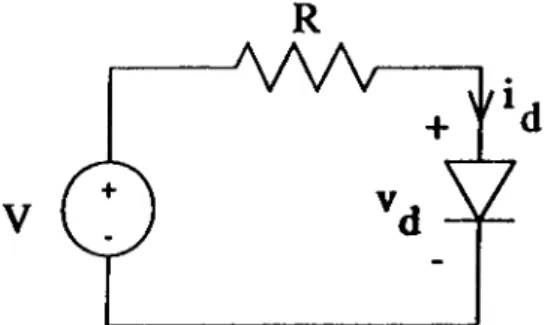
Figure 2.6: Simple Diode Circuit
Nonlinear Case
Consider the diode circuit example as shown in Fig. 2.6, a manual approach to find the current through the diode would be as follows:
td
=V - v ¿
R
id
= -1
)Graphically, it is seen that the solution can be found by load line method [11]. Computationally, some iterations have to be made to reach the solution. An iteration simply consists of assigning a guess for the solution, initieJly. Then solving the equations above, the error — the difference between the guess and the result— is obtained. According to the error, the guess is revised. Same steps are repeated until the error is sufficiently small. One common way to realize this type of iteration is the Newton-Raphson algorithm which will be pointed out later in this section.
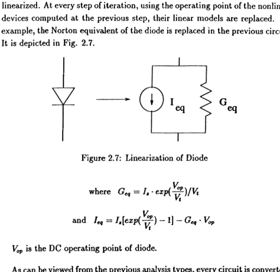
To handle these operations on the computer, nonlinecir devices have to be linearized. At every step of iteration, using the operating point of the nonlinear devices computed at the previous step, their linear models are replaced. For example, the Norton equivcdent o f the diode is replaced in the previous circuit. It is depicted in Fig. 2.7.
G
eq
Figure 2.7: Linearization of Diode
where Ge, =
I, ■ exp{-^)IVt
and / ^ = / . [ e x p ( - ^ ) - l ] - G „ - V ;op
Vop
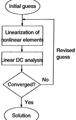
is the DC operating point o f diode.As can be viewed from the previous analysis types, every circuit is converted to its equivalent linear form. Therefore, the solution is obtained by performing linear DC analysis. All ainalyses can be based on the solution o f the linear equivalent of the circuit.
N e w to n -R a p h s o n A lg o r ith m
Newton-Raphson iteration is the most importamt part o f DC cind IVansient analyses. The Newton-Raphson algorithm seeks to solve the nonlinear equation
f { x )
= 0iteratively by successive solution o f a set of linearized approximations to this equation.
The flow diagram o f the Newton-Raphson (NR) algorithm is shown in Fig. 2.8. Every nonlinear device is searched in every step of NR iteration, and linearized гw:cording to the solution coming from the last step. As an example, linearization of diode is described in the previous part and shown in Fig. 2.7.
Figure 2.8: Newton-Raphson Algorithm Flow Diagram
Then, the equations are formed according to the new circuit — which is linear— , and solved until two successive solutions are sufficiently close.
Newton-Raphson iteration may not always converge. Accordingly, there heis been various modifications on the pure form to help convergence. One way that is tried at Bilkent University is using piece-wise linear (PWL) models [12]. The NR algorithm may fail if it caji not visit the right set of lineM regions o f the elements that the real solution lies. In PLAWE, a possibility of changing region randomly is included, to assure convergence. Eventually, the right set of regions where the solution lies will be found, even if there is a chain of wrong solutions.
A special treatment about diodes is taken into consideration to help conver gence in this work. Diode model is modified as depicted in Fig. 2.9. To avoid numerical errors and lots of iterations — which au-e a result of the exponential behavior— , the function is considered as a line that is tangent to the ideal one at the point where uj = 1.0 , for
vj >
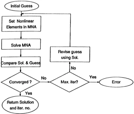
1.0. It is shown as a dotted line in Fig. 2.9. Such modifications on the models of some nonlinear devices must be done to help Newton-Raphson algorithm to find the solution easier.The flow diagram of nonlinear version of DC Analysis is shown in Fig. 2.10. The loop is adso called Newton-Raphson iteration.
o
+ ' ' 'd
V
Figure 2.9: Diode Model
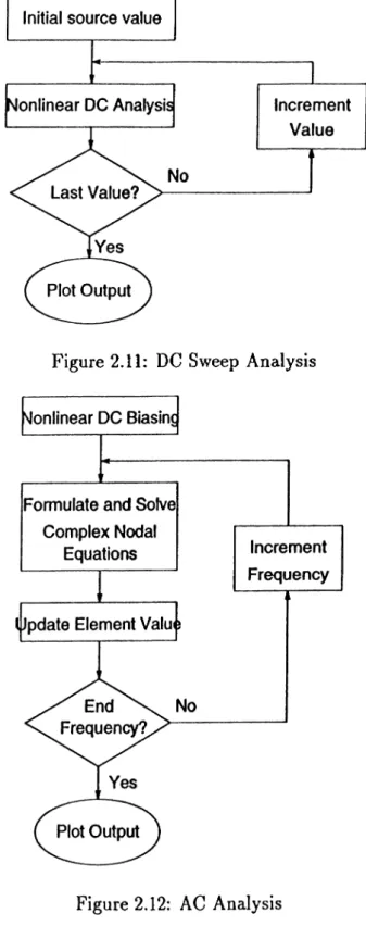
Another type of analysis is DC sweep analysis. It is performed to examine the effect of a source. The value o f an independent source is swept in a range, then the solution is found as a function of this varying input. This calls DC analysis part with the new value o f the input at every step. The flow diagram is shown in Fig. 2.11.
The flow diagrams of AC ancdysis and nonlinear version of TViinsient anal ysis are shown in Figs. 2.12 and 2.13, respectively.
Revised guess
The method Asymptotic Waveform Evaluation (AWE) can be employed in AC and Transient analyses. This is an approximation o f response of linear circuits by a reduced order of polynonaial rational. It will be mentioned in Chapter 3, in detail.
2.3
Matrix Setup
As it has already been remarked in the previous section, every type o f analysis can be handled by replacing the circuit with its DC equivalent and performing linear DC analysis. That is, the core of the simulator is the solution of set of linear equations. This approach leads us to matrix concept, as linear equations can have a matrix form.
The equations of the sample circuit in Fig. 2.2 can be rewritten in terms of the unknowns, ei,C2 and
iy
as follows:Gl · Cl + —G\ · + ~Gl' Cl T {G\ T G2) · C2 Cl
- t v =
0
0
V
It is apparent that these equations can be formed as a matrix equation Gl - G l -1 - G l {Gl + G2) 0
1
0
0
Cl ‘ 0 ‘ C2 0 «VV
Solving this matrix equation yields the results.
Now concentrate on how a matrix belonging to a certain analysis is created.
Types of matrix formulation
There axe two common formulations. One is Nodal Analysis and the other is
Sparse Tableau Analysis
(STA). [11] There is cdso Loop Analysis, which is not generally used in circuit simulators. Most common usage of Nod£il Analysis is its modified version, which will be referred as Modified Nodal Analysis (MNA).[2]
In PLAWE [6], STA formulation is used. STA is easier to setup, but it produces larger sized matrices and requires more memory space than MNA, which also decreases the efficiency of the solvers, esjjecially for circuits having lots of elements.
Modified Nodal Analysis
Modified Nodal Analysis is used to formulate a circuit as a form of matrix equation. As the name suggests, it is the generalization of NodaJ Analysis, which can only cope with voltage controlled elements. MNA was introduced to deal with problems «issociated with any other type of elements, such as voltage sources and current-controlled circuit elements. It includes KCL and Brajich Constitutive Relations. So far, many types of matrix formulations are used in the circuit simulators, but MNA has become the most widely used one. An industry standard, SPICE also uses MNA.
The matrix equation formed by using MNA can be partitioned as:
> n
E '
e
’ j
F
D
i
.K
where K is the nodal admittance matrix, the contribution of each element is inserted into this matrix, as long as currents can be expressed as explicit functions of voltages.
E
is the incidence matrix of the voltage sources and current-controlled elements of the circuit.F
andD
(can be called as Branch Constitutive Rela tions) contain the contributions of the circuit elements which are not voltage controlled.The vectors
J
andK
represent the contributions of the excitation sources, i.e., independent current and voltage sources.Setting up M N A Matrix
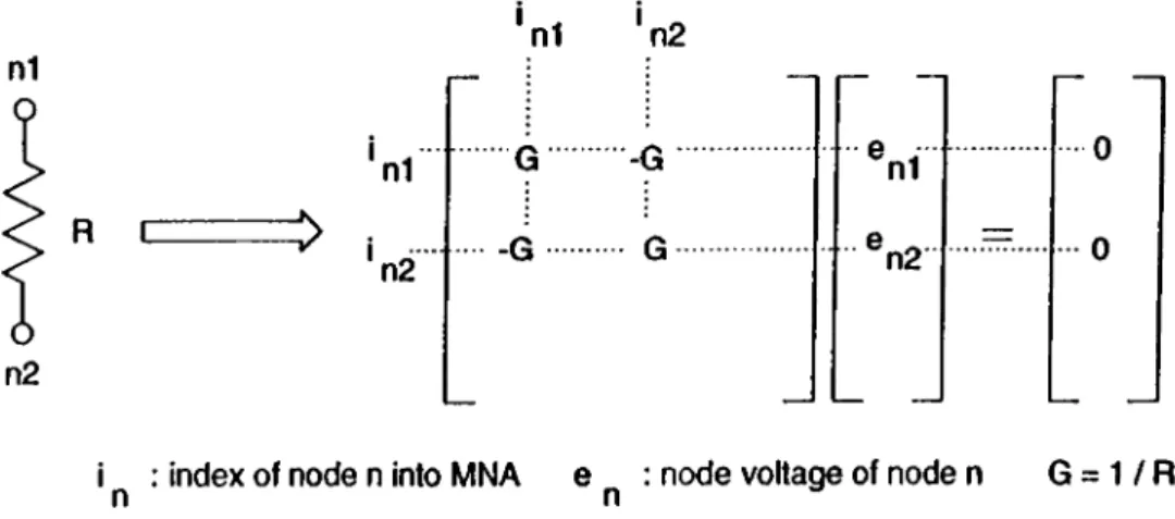
The main advantage of dealing with matrix type of equations is that the contributions of all the individual elements can be inserted directly at appro priate places in the matrix. Therefore, setup functions of every device can be written independently. These setup functions of the elements and devices are called “stencils” . In Fig. 2.14, the contribution of a resistor in MNA matrix is depicted. The stencils implemented in this work are given in Appendix C.
In every step, setting up MNA and destroying it after finding the solution takes a lot o f time. Keeping the old MNA and adding it only the differences in the values of the devices saves time. Therefore, every device has an initial setup part that forms the MNA at the first step and next-step parts that introduces the changes in their values. For example, the resistors are only visited at the first step, since their values do not change throughout the analysis. However, this method of matrix setup may cause numerical errors if the entries of matrix are near zero or the matrix is ill-conditioned.
R C n1 ' n1 ' n2 i> , ... n2 G -G G G 'n i ... e n2 0 0
i : index of node n into MNA e : node voltage of node n G = 1 / R
n n
Figure 2.14: Stencil of a Resistor
Since every analysis introduces a different method, different functions are written to handle them. Therefore, an analysis should visit appropriate setup functions to build up the MNA matrix. However, for example, in the DC sweep analysis, since capacitors have no effect on the result, no function is
implemented in DC, for capacitors. Adding a new analysis means writing these functions (stencils) for every device and calling them according to the method employed. Addition o f a new analysis type is described in Chapter 3, Section 5.
2.3.1
M a trix S olvers
In SIMLIB, real and complex matrix solvers are used. Using the complex library of C + + , converting a real matrix package into a complex package is very simple, therefore doing operations on complex numbers is the same as the real numbers, which is an adveintage of C + + . First a sparse matrix package and a non-sparse matrix package is written and then their complex versions are created.
Sparse Matrices
The resulting matrix o f a Nodal Equation set of an electronic circuit, has in general lots of zero-valued elements, because every node is not connected to every other node. Such matrices are called Sparse Matrices. Moreover, for much larger circuits, the MNA or STA matrices are much more sparse. Even the percentage of the zero-valued elements reaches to 99%. Sparse Matrix Packages take advantage o f this property; reduce storage requirements; and reduce the number o f floating point operations entmled for LU-factorization and FBS. [3]
Non-sparse Matrix Solvers
In the moment analysis part,(explained in Chapter 3, AWE method) non- sparse matrices are used. Since the matrices are non-sparse, using sparse tech niques introduces lots of overheads. Therefore, creating all the elements of the matrix and performing operations on it is a better way. It doesn’t have to use indexing methods, managing memory is simpler.
All the matrix packages used for this work are explained in detail in Ap pendix D.
Chapter 3
ALGORITHMS AND
IMPLEMENTATION
In this chapter, the <ilgorithms of the input parser, analyses and AWE technique are listed and explained so as to introduce how the program works. In the fourth section, the implemented parts are mentioned. Finally, modification of the existing library is explained with two examples in the last section.
3.1
Algorithm of Input Parser
1 Initialize the “circuit” * structure. That is, open field, set the variables to their initial values.
2 Start with the first line of the input file consisting the circuit definition for performing the following step.
3 Check the first character on the current line. If it is valid, call the “first-pass” function of the corresponding class, else print the error mes sage and exit.
Note :
These functions are written according to the style of definition of each device. The node names are inserted into node tables, (table structure is explained in Appendix D) to be able to convert them into index numbers in the step. And errors in the declarations are reported. *The reader may look at the Appendices B and C for the database and matrix setup functions to check the quoted words.4 Read the next line and repeat step 3 until end of file is reached.
5 Create field in the memory for the devices declared by calling “cre- ate-field” functions of them. The size, that is the number of the devices are counted in step 3.
6 Go back to the first line of the input deck.
7 Check the first character on the current line. If it is valid, call the “sec ond-pass” function of the corresponding class, else print the error message and exit. In these functions the parameters are reaxl and inserted into their corresponding fields.
8 Compute the size of circuit and matrix according to the analysis type to be applied. The size is the sum of number of nodes, voltage sources and current-controlled elements.
9 Return the “circuit” structure which contains device classes and the op tion cards and type of analysis that will be performed.
3.2
Algorithms of Analyses
Assuming that the input parser is called, the data is ready in the “circuits” structure.
DC sweep analysis
1 The source -whose DC value will be swept in a range- is set to the initial value.
2 The solution array is initialized to zero. The solution array is the vector of unknowns of the MNA function.
3 Call “set-MNA” functions^ (stencils) of each device, except capacitors and nonlinear devices.
4 Call Newton-Raphson iteration function, which is outlined as follows: 4.1 Add the linearized models of the nonlinear devices into MNA by
calling “set-MNA” functions of them. (These functions require op erating point, which is extracted from the solution array.)
4.2 Solve the resulting matrix equation.
4.3 Compare the old solution array with the new result. If the difference is not sufficiently small, then assign solution array the new result and goto step 4.1.
5 Print out the desired entries of the solution array. This is defined in the .print card of the input deck (See Appendix A ), and the “circuits” structure consists this information.
6 Increment the source value. If last value is not reached, then goto step 4. 7 Print out the statistics. (Solution time, number of iterations, etc.)
AC Analysis
In AC analysis, the Matrices are complex, so the functions for this analysis uses complex sparse matrix package.
1 Set frequency to the start value.
2 Call “set_CMNA Jncond” functions of each device. The complex MNA matrix will be formed.
3 Solve the complex matrix equation.
4 Print out the desired entries of the solution array, in the given format (magnitude, phase, real or complex part).
5 Increment frequency. If it is the last value, then stop. 6 Call “set_CMNA” functions of each device. Goto step 3. 7 Print out the statistics.
Transient Analysis
1 Specify whether the circuit contains nonlinear elements or not. 2 Call “set-MNA jn con d ” functions of each device.
3 If the circuit is linear, solve MNA equations, else call Newton-Raphson to get the solution. This yields the initial condition.
5 Destroy MNA, ajid call “set.MNA” functions of each device, except dy namic elements. MNA is created again since the size is changed because of the initial conditions of capacitors and inductors has introduced a larger circuit at the second step. This time the circuit is smaller.
6 Increment time.
7 Call “set_MNA” functions of dynamic elements. Norton equivalents of capacitors and inductors are inserted according to the trapezoidal ap proximation.
8 If the circuit is linear, solve MNA equations, else call Newton-Raphson to get the solution.
9 Print out the desired entries of the solution array.
10 If the end of analysis time isn’t reached, then goto step 6. 11 Print out the statistics.
Some example circuits and print-outs are given in Appendix F.
3.3 Algorithm of AW E Method
AWE (Asymptotic Waveform Evaluation) technique is a new approach which is used in timing analysis of RLC interconnect trees. It approximates time response of a state variable by less number o f exponentials, and frequency response by a lower order polynomicd rational. This method finds moments of the actual circuit (integral or derivative) and matches them to the polynomial. New revised versions of AWE are used to find nonlinear circuit solutions, and it is adapted to frequency analysis.
For the theoretical details of AWE see the references [5], [13], [14], [15],[16], [17],[18],[19],[8]. Now, concentrate on the computational algorithm to simulate a circuit using AWE :
1 2q-l moments axe needed. These could be integral moments, derivative moments or a combination of them.
Integral momenta :
First, find the DC operating point of the circuit (open circuit capacitors, short circuit inductors). Call the capacitor volt ages and inductor currents ml*j moments. (A superscript C is used for capacitor moments and L is used for inductor moments.) Then1. Set independent sources to zero.
2. Replace capacitors with current sources of value
C · m f
3. Replace inductors with voltage sources of value
L
· m f4. Compute the resulting circuit. The voltages across capacitors are m[^j, and the currents through the inductors are m,^j.
5. Return to step 2., and find the next moment until / reaches the last index of integral moments to be calculated.
Denvative moments
: This time replace capacitors and inductors with voltage and current sources respectively. The values are set to their initial conditions. Call the solution (capacitor currents and inductor voltages)moment.
1. Set independent sources to zero.
2. Replace capacitors with voltage sources of value
m^/C
3. Replace inductors with current sources of value
mj^/L
4.
Compute the resulting circuit. The currents through capacitors are m^_j, and the voltages across the inductors гu·e5. Return to step 2., and find the next moment until
k
reaches the last index of derivative moments to be calculated.Note that the index of the first integral moment is 0 and the others follows as 1, 2, 3, . . . , the index of the first derivative moment is -2 the others follows as -3, -4, -5, . . . . m _i is the DC solution of the circuit. So it is neither called integral nor derivative moment.
2 Using these moments form the matrix equation as, (supposing there are n integral and m derivative moments, (m + n + 1) should be even)
-m -n-3
-m -n-3 (*)m (,_i) (*)m , (*)m (,+i) (*)m ,mm-i
Oq (*)m , (*)"*(7+l) 02 (*)m(,+2) m + n - f l j / \where
q
= ---and (*) — 1i f index < —I
1otherwise
The solution is the coefficients of polynomial,
C"(A) = qq T fliA T Q 2 ^ ■{■··· T Qj-iA^ ^ T a*
3 The reciprocгıl o f the roots of this polynomial gives us the approximate poles of the state variable
x,
wherex
can be representedas,
x{t)
= X ;Pj
are the poles, andkj
are the corresponding residues.4 Obtaining the Vandermonde matrix we can find the residues of the poles,
i/k = mi ■ A f" A*"" ··· V ■
t/
= Ar"+* \-n+lA2
. . . and m i = -m _ n -2x r
\r^
···x r
.where A,· ’s are the roots of C'(A), and m/ is formed by the first lower-order q moments.
5 The solution of the matrix equation in the fourth step yields the residues. Then the approximation for
x{t)
is found.For this method, a complex polynomial root finder and a moment class is implemented. The flow diagrams are given in Figs. 3.1 and 3.2.
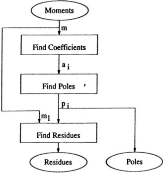
Figure 3.1: Diagram of the Polynomial Root Finder
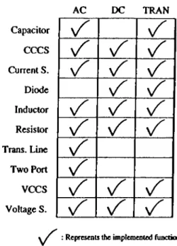
SIMLIB is a collection o f library functions for electronic circuit simulation. As it cam be viewed from the chart in Fig. 3.3, some of the circuit elements and their analysis functions are implemented. One can fill the blcinks or add a new row, which means adding a new device, or add a new column, which means adding a new analysis type. This is explained step by step in the next section.
3.4
Implementation
AC DC TRAN Capacitor CCCS Current S. Diode Inductor Resistor Trans. Line Two Port VCCS Voltage S.: Represeols the implenieoled fuoctiaos
Figure 3.3: Analysis vs. Elements
Besides, some routines that control the flow of the prograun are imple mented. One o f these routines checks the “jobs” structure, which is embedded in “circuits” structure ^ and calls the corresponding functions. That is AC, DC or transient analyses. Then in these analyses the stencils of the devices are called.
Also matrix packages which is used to form a matrix equation and to solve this are implemented. The table package which is used for indexing in the input parser part is written. Both packages are implemented by Ogan Ocah. The usage of them are given in Appendix D.
The remaining functions and their usage are given in Appendix E. And some of the source listings are added.
One of the requirements of this work is to create an easy-to-modify library. This property will be described with an example in this part. Examining Appendix B and E, directory structure and variable declarations will be helpful before going into details of the program.
3.5
Modification
3.5.1
Adding a New Device
In this part, a “capacitor” as an example to a new device is described.
1. Write “capacitor” class.
(a) Write the include file of the class, which declares the variables and the functions related to the element. Add it to the file “simlib- home/include/twoterm.h” . class cap { int anl»*n2» count; doubla aval, ♦ ic, aIeqp,aGeqp; // nod· indic«s
// used as internal pointer // value of the capacitor // initial condition
// equivalent 1,0 at the previous step public:
int capno; // total nuiber of capacitors in the class c a p O ; // construction
‘c a p O ; // destruction void first.passdncirc ecurcirc); // Input void create.fieldO; // Parser void second_pass(incirc ecurcirc); // Functions
void set.NIACdouble esol,double dT); // Transient an. stencil func. void set.CNIA(double freq); // AC analysis stencil func. void list.allO;
>;
(b) Write the class functions in a file “simlibhome/source/devdir/capacitor.C” .
•include "includes.h" /•♦eeee
capacitor class definitions
cap::cap() // initial declaration
{
capno^;
count^O;
>
cap::'cap() // destruction function
{
// cout << "Cap. destroyed!";
>
void cap;:first_pass(incirc acurcirc)
/♦♦*♦
usage : C x x x x u nodel node2 value <ic*noAber> no. of paraneters of capacitor should be at least 4. global variables;
uord.nuM : no of uords on a line, vord_list[i] : the i ’th oord on the line. nodel and node2 are added to the **nodetable*’. capno is increaented at every call.
eeee/ <
if (vord.nua<4) {
sprintf(aess,"Error in capacitor Is !\n"»vord.list[0]); erroraessO ; } else { curcirC'*>nodetable .putsyaCuord.listCl]) ; curcirc->nodetable.putsya(vord.list[2]); capno-M·; > >
void cap: icreate.fieldO
{
nl « nev int[capno]; n2 ■ nev int[capno]; val * nev double [capno] ; ic ■ nev double[capno]; leqp ■ nev double [capno] ; Qeqp » nev double [capno] ;
}
void cap::s6cond.pass(incirc acurcirc)
{
int iBcount;
// using the sya table *^nodetable’* insert values nl,n2.
// nl and n2 are index nuaber vhich vill be used to point to an HIA entry. nl[i] " get.index(curcirc,vord.list[l]);
n2[i] ■ get.index(curcirc,vord.list[2]):
// read.nua returns 0 if there’s an error in typing of the value, // or converts the string into a double.
if(!read.nua(vord.list[3],val[i])) {
>
// if th«r«^8 an error in i.c. value it is taken as 0. ic[i]«0.0;
if (!strc*p(gord.list[4] ,”ic··) fti (vord.list[5] [ 0 ] » ’« >)) if(!read.nuaCvord.list[6],icCi])) ic[i]»0.0; •xit(l); OeqpCi] ■ count++; leqpCi] « 0.0; >
/♦♦♦* This function is used for transient analysis ♦♦♦♦♦/ void cap::set.HIA(double asol»double dT)
<
double Vop»Geq,Ieq,Iadd,Gadd; for (int i=0 ; i<capno; !+♦)
{
Geq « (2.0sval[i])/dT;
0.0) At (leqpCi] ««0.0)) { // At the first step Geq e ic[i] ; // these will be
// evaluated according to the ic value // For the next steps
// leq and Geq will be
It calculated using Vop
ft found at previous step if ((GeqpCi] *»
ladd ■ leq ■ Ieqp[i] Gadd ■ GeqpCi] « Geq ; > also { if (nl[i]>-l) Vop ■ sol[nl[i]]; if (n2[i]>-l) Vop -* sol[n2[i]]; ladd ■ Vopa(Geq+GeqpCi])-2eIeqp[i] ; leqpCi] +■ ladd ;
Gadd ■ Geq - GeqpCi]; GeqpCi] * Geq;
>
if (Gadd!-0.0) { if (nlCi]>-l)
ins.PKH»nl Ci] .ni Ci] .Gadd) ; if (n2Ci]>-l) ins.N(H,n2Ci].n2Ci].Gadd); if ((nlCi]>-l) At (n2Ci]>"l)) { ins.H(H,nlCi].n2Ci].-Gadd); ins.H(H.n2Ci].nlCi].-Gadd); >
// Stencils, see appendix C
i f (nlC i] >-l)
ins.b(b,nlCi].ladd);
i f (n2Ci]>-i)
ins.b(b.n2Ci],-Iadd);
>
/eee«#e XC analysis part ♦·♦♦♦♦♦♦/ void cap::set.CraiA(dooble f)
<
for (int i»0; Kcapno; i’*·'*·) {
Qadd ■ co»plax(0,2*PI*f*val[i]); // AC equivalent inpediance of cap.
inB.H(CH,nl[i],nl[i],Gadd); ins.H(C«.n2[i].n2[i].Qadd); inB.H(CH,nl[i].n2[i].-Oadd); ins.H(CN.n2[i].nl[i].-Qadd):
// Stencil of cap.
/♦♦♦♦♦♦♦ listing of all capacitors in the class ♦*♦♦♦♦*/ void cap::list.all()
{
for (int i»0; Kcapno: i-f-+)
cout«*'cap["«i«··] - ••«nl[i]«".''«n2Ci]«'*.val="«valCi]«"\n” :
>
So the capacitor class implementation is completed.
2. Add the capacitor class to the “circuit” structure, which is explained in Appendix B. It is declared in “simlibhome/include/inp.h” .
typedef struct inckt { char esubna··: res eresistor: vs •Tolt:
cap «capacitor: // should be added.
} incire:
3. The input parser functions should be called from the input parser module. It is the file “simlibhome/source/input/device.C” .
void first_pass(incirc *curcirc) {
curcirc“>capacitor ** new cap; // should be added.
while (parse_file(infile>) { lineno++;
switch (word_list[0][0]) {
case *c* : //
case : //
curcirc->capacitor->first_pass(curcirc); // should bo added,
break; //
void croato_'fioldsO {
temp->capacitor->croato_field(); // should bo added. >
void second_pass(incirc »curcirc) {
while (parso_file(infile)) { linono++;
switch (word_list[0][0]) {
case ^c^ : // should bo added,
case :
cureirc“>capacitor->socond_pass(cureire); break;
4. The transient analysis function is “simlibhome/source/analyses/tran.C” . This module calls “set_MNA_dyn” function, which calls the transient analysis stencil functions of all the dynamic elements. “set_MNA.dyn” is in the file “simlibhome/source/methods/mna.C” . “set_MNA” function o f the class capacitor should be added in here.
void sot.MIA_dyn(double ♦sol)
{
circ->parent“>capacitor->8et_MIA(sol,circ->job.step); // should be added.
5. The AC analysis function is “simlibhome/source/analyses/ac.C” . This module calls “set_CMNAJncond” and “set.CM N A” functions, which are the complex version of set_MNA. These functions are in the file “simlib- home / source/methods/mna. C” .
void set.CMIA.incondO {
circ->paront->capacitor->sot_CHIA(circ->job.start); // should be added. // initial value
>
void set_CMIA(double f)
{
circ->paront->capacitor->sot_CMIA(circ“>job.step); // should bo added. // next step additive value
}
After the completion of the steps above, capcicitor is added to the simulator for transient and AC analyses. Note that it is easier to copy one of the existing device classes and make the changes on this file.
3.5.2
Adding a New Analysis
1. To parse the analysis declaration in the input deck a “read.dc” function is added to the class “jobs” . Include file is “sim libhom e/include/jobs.h” .
class jobs { public:
void read.dcO;
};
And write the function in file “sim libhom e/source/input/jobs.C” .
void jobs::read_dc()
{ /♦♦♦
usage: .dc vs.nane start_value stop.value step.value
***/
if (word_num<5) {
strcpy(mess,"Error in .dc card! (check number of words)\n"); errormessO ;
>
dcok=l; // dcok flag is set TRUE,
// meгLns DC emalysis will be performed strcpy(vsname,vord_list[1] );
if (!(read_num(vord_list[2],start) kk
read_num(vord_list[3],stop) kk
read_num(vord_list[4],step)>) {
strcpy(mess,"Error in .dc card! (check numbers)\n"); errormessO ;
}
Note that vsname, start, stop and step are public variables o f jobs. See Appendix E for details.
2. Reading the analysis card should be added into the “first.pass” function of the input parser .
void first_pass(incirc »curcirc)
{
if ( !strcmp(word.li8t[0],".dc")) { circ“>job.read_dc();
b r e a k ;
3. The MNA setup functions (stencils) should be added to the device classes that are supported in the new analysis. See Appendix C for information about stencils.
For example, “set-M NA” function for a resistor will be written as :
void r e s ::set.NlA()
{
if (resno<l) return; int n i ,nj;
double ival;
for (int i=0; i<resno; i++) { ni = nl[i]; // node indices nj » n2[i] ;
ival » 1 .0/val[i]; // G = 1/R
ins_N(N,ni,ni,ival); // stencil for resistor ins.H(H,nj,nj,ival);
ins.M(N,ni,nj,-ival); ins_H(M,nj,ni,-ival);
4. Write the “set_MNA” function in “sim libhom e/m ethods/m na.C” which calls the stencil functions of the devices.
void s e t . N I A O
{
int size;
size * circ->totalsize; //get the size of the NIA natrix // This size is set in the input parser
N * spmcreateCsize»size); b » neu double[size];
for (int i»0;i<size;i··-··) b[i] * 0.0; circ->parent->reAistor->set_HIA(); circ->parent->volt->set.HIA();
c i r c “ >parent->VCCS->set_MIA();
5. Then write the analysis function which calls these MNA setup functions. Analysis function of DC part is “simlibhome/source/analyses/dc.C”
tinclude “includes.h" tinclude “mna.h"
void do.dcsveepO
{
double ^sol,esoll,*sold,*soli;
int vsindex,iterno=l ,totaliter=0,itershow=circ->job.shouiter; double tim^vval;
// Get the index of the voltage source vhose // value will be swept
if ((vsindex =* circ->parent->vstable(circ->job.v8name))<0) { c e r r « “Error in .dc card vs is not defined ! \n'';
exit(l);
>
sol = new double[circ->totalsize] ; soli “ now double[circ->totalsize] ; sold = new double[circ*->totalsize] ;
for(int j=0;j<circ“>totalsize;j++) 8ol[j]=sold[j]=soli[j]=0.0; // place of vs in NIA is no. of nodes + vsindex
vsindex +“ circ->parent“>nodetablo.nofsymO ;
circ“>job.outnames[strlon(circ->job.outnaines)] * *\0’;
cout«·' VoltageC’«circ->job.vsnamo«'*) *'<<circ->job.outname8; tim = c l o c k O ;
set.NIAO; j=0;
for (vval = circ->job.start; vval <* circ->job.stop;wal += circ“>job.step)
{
b[vsindex] = vval ;
for(j=0;j<circ->totalsize;j++) 8oli[j]=sol[j]; soli > VewtonRaph8on(sol,itemo);
sol » new double[circ->totalsize]; for(j»0; j<circ->totalsize;j+···) { 8ol[j]=8oll[j];
>
totaliter +« iterno; // counts the iter no. output(vval,sol);
if (itershow) cout<<iterno;
c o u t « " \ n " ;
>
cout<<"\n total iteration » "«totaliter; tim » c l o c k O - tim;
c o u t « " \ n d c sweep time="<<tim/1000000<<" sec.\n"
>
“NewtonRaphson” function is implemented in file “simlibhome/methods/nr.C” . This funtion calls “set_MNA_nonlin” function, which calls the MNA setup functions of nonlinear elements. Of course, such special functions should be designed and added by the programmer according to the methods used.
Chapter 4
CONCLUSION
In this thesis, some library functions to develop electronic circuit simulators are implemented. The collection of these functions is called as SIMLIB. The main property o f SIMLIB is that modifications such as addition of new analysis types and methods can be applied easily. Besides, although this implementetion covers only some circuit elements, any device can be added to the simulation library with a little effort. To describe such additions and modifications, an example is given.
SIMLIB consists of an input parser, sparse and non-sparse matrix packages, a symbol table package, AC, DC, transient analyses, moment matching by using the AWE technique and some device classes including most commonly used ones, linear elements, capacitor, inductor, diode, transmission line, etc.
The programs are written in C + + , which is an object-oriented program ming language. The object-oriented feature has provided to write the program in a modular way. This modularity enables other programmers to get familiar with the program easily.
Since the aim was to build a development tool rather than to write a very fast or exteremely accurate simulator, simple models of the existing devices have been used, and the implementation has been restricted to a limited set of devices. As a result, the library can be easily modified and extended to include other devices.
The future work should concentrate on constructing new simulators in which some novel methods are examined. Applying new methods and ex tending the types of analyses, including new devices to SIMLIB, modifying the modules to make the program work faster and more accurately are some of the issues left to be investigated.
Appendix A
SIMLIB M AN U AL
It is almost the same as SPICE input deck. There are some differences which the users should be careful about. All the nodes can be either numeric or alphanumeric. There’s no value checks for the time being.
A .l
Elements
In the following, the formats of declaration of elements are listed.
1. Resistors
Rxxxxxx [nodel] [node2] [value] 2. Voltage Sources
Vxxxxxx [node+] [node-] [value] 3. Current Sources
Ixxxxxx [node-f] [node-] [value] 4. Capacitors
Cxxxxxx [node-f] [node-] [value] 5. Inductors
Lxxxxxx [node-b] [node-] [value] 6. Voltage Controlled Current Sources
7. Voltage Controlled Voltage Sources
Exxxxxx [node+] [node-] [controlling_node-|-] [controlling_node-f] [value] 8. Current Controlled Current Sources
Fxxxxxx [node-f] [node-] [Vjiame] [value] 9. Current Controlled Voltage Sources
Hxxxxxx [node-f-] [node-] [V_name] [value] 10. Diodes
Dxxxxxx [node-f] [node-] <is=[is_value]> <vt=[vt.value]> 11. Transmission lines
Txxxxxx [nodel] [node2] [node3] [node4] Z0=[value] F=[value] NL=[vaJue] or
Txxxxxx [nodel] [node2] [node3] [node4] C=[value] D=[value] L=[value] 12. Two-ports
Yxxxxxx [nodel] [node2] [node3] [node4] ( y l l ) (yl2 ) (y21) (y22) Where yxx are the elements of admittance matrix ;
r =
y ll yl2
y21 y22
In two port representation (yxx) will be written as
((Po Pi
P2-Pn){qo qi i2-9m))where
yxx =
_ (po + Pi ■ W + P2 · + ... + Pn · w")(qo + qi ■ tv + g2 · + — + 9n ·
(Note that a ’-H’ sign at the beginning will add the current line to the previous line.)
A . 2
Analyses
1. DC analysisUsage : .dc [V-name] [start-value] [stop-value] [step-value] 2. Transient analysis
Usage : .tran [step-time] [stop-time] 3. AC analysis
Usage : .ac [start Jreq] [stopJreqJ [step_freq]
A .3
Output formatting
1. Printing :
Usage : .print v(node) i(V_name)
( if only V or i is written magnitudes of the values axe printed. other options :
vm,im : magnitude ; vp,ip : pha^e ; vr,ir : real part ;
vi,ii : imagimary part .) 2. Options :
Usage : .options <optionJist>
( list : lists the circuit (to see how the input deck is parsed),
printmb : prints the MNA matrix and the source vector in every step for tracing what happens during the analyses (not recommended for large circuits.
Appendix B
DATABASE
B .l
Global Declarations
The most important global variables are the circuit structure and the matrix structure. See Appendix E, Section 2 for a detailed list.
B.1.1
Circuit
The circuit structure contains
• Device classes (includes every data and function related to) • Lookup Tables (which are defined as classes) for indexing • Models for the devices
• Jobs to be performed, style of the output • Subcircuits
B .l .2
Devices
Devices are implemented as classes having required variables and functions. A device typically contains :
Device #1 Device #2 ■ • ■ Device #n Device Pointers Node Table — > other Tables s. Lookup Tables Next INCIRC Variables INCIRC Structure * N INCIRC Jobs Models Indexes Variables CIRCUITS Structure
• Its occurance number in the subcircuit
• Node numbers used as the indexes into the MNA matrix • Device values (e.g. resistence value for a resistor)
• Construction and destruction functions
• Functions for input parsing and circuit creation
• Stencils for MNA formulation (for each type of analysis) • A listing function
Examples for two-termincJ devices:
• Capacitor • Diode • VCCS • CCCS • Inductor • Voltage Source • Current Source • Resistor
Examples for four-terminal devices :
• Transmission Line • Two port
B.2
Jobs
Jobs is the class responsible for reading the cards of an input deck. It sets the variables indicating whether a DC, AC or Transient analysis will be performed. It reads the model cards and also the option cards. It contains the format of the output style.
B .3
Subcircuit
This is held by the recursive structure of the "circuit” . In every cir c variable there’s a field of pointer pointing to another cir c structure.
B .4
Matrix
There iire four Matrix Packages used in this program:
• Real Sparse Matrix Package • Complex Sparse Matrix Package • Real Non-Sparse Matrix Package • Complex Non-Sparse Matrix Package
All o f them are implemented as classes in C+-|-. In Appendix D the usage and the properties are explained.
Appendix C
STENCILS
In this part, the stencil functions of the elem
ents are listed.
Representation:
The following matrix equation is tried to be constructed.
Mx = b
where M is an
n x nmatrix and x and b are vectors of length n.
n, is the index of node i of the element for the M
NA matrix.
M[n,, nj]+ =
v a lu em
eans adding
v a l u einto the entry of matrix M.
=
v a l u em
eans adding
v a lu einto the n,·,
n jentry of matrix M.
1