THE FUNDAMENTAL GROUP OF A GENERALIZED TRIGONAL CURVE
Alex Degtyarev
Abstract. We develop a modification of the Zariski–van Kampen approach for the computation of the fundamental group of a trigonal curve with improper fibers. As an application, we list the deformation families and compute the fundamental groups of all irreducible maximizing simple sextics with a type D singular point.
1. Introduction
1.1. Principal results. We attempt to develop a modification of the classical Zariski–van Kampen approach [18] suitable to compute the fundamental group of a generalized trigonal curve, i.e., a trigonal curve with improper fibers, at which the curve meets the exceptional section. A similar question was addressed in [11], where the only improper fiber was ‘hidden’ at infinity. Here, we consider the case of arbitrarily many improper fibers (up to two in the applications).
The basic tool used in Zariski–van Kampen’s method is the braid monodromy related to an appropriate pencil. This concept was introduced by O. Chisini [4], [5], O. Zariski [27], and E. R. van Kampen [18], and the term itself is probably due to B. Moishezon [22], who has also introduced explicitly such notions as the monodromy at infinity, braid monodromy factorization, and Hurwitz equivalence. For more details on the braid monodromy techniques in general and its usage in the computation of the fundamental group and other related invariants, as well as for the recent developments in the subject, we refer to the excellent recent surveys by Vik. S. Kulikov [20] and A. Libgober [21]. Note though that in this paper we are not concerned with the Hurwitz equivalence and merely use a certain modification (see next paragraph) of the braid monodromy as a computational tool. The Hurwitz equivalence of braid monodromy factorizations of a given element, even B3-valued
and even those of algebro-geometric origin, seems to be a rather delicate subject; for some new results and further references, see [16].
In order to keep the braid monodromy well defined, B3-valued, and easily
com-putable via skeletons (see Subsection 3.6), we pass to the associated genuine trigo-nal curve and introduce the concept of slopes, which compensate for the improper fibers. We compute local slopes (Subsection 3.5), study their properties, and discuss the modifications that should be made to the braid relations (3.4.4) and relation at infinity (3.4.6) in the Zariski–van Kampen presentation of the fundamental group, see Corollary 3.4.7.
2000 Mathematics Subject Classification. Primary: 14H45; Secondary: 14H30, 14H50.
Key words and phrases. Plane sextic, fundamental group, trigonal curve, dessin d’enfant.
Typeset by AMS-TEX 1
As a simple application, in Subsection 3.7 we recompute the fundamental groups of irreducible plane quintics with a double point. (These groups were originally found in [7] and [2], but the computation via trigonal curves is much simpler and more straightforward; it could easily be computerized.)
1.2. Plane sextics. A more advanced example is the case of irreducible plane sextics with a type D singular point.
Recall that a plane sextic C ⊂ P2 is called simple if all its singular points are
simple, i.e., those of types Ap, Dq, E6, E7, or E8(see e.g. [1] for the notation). The
total Milnor number µ(C) of a simple sextic C does not exceed 19; if µ(C) = 19, the sextic is called maximizing. Maximizing sextics are rigid: if two such sextics are eq-uisingular deformation equivalent, they are related by a projective transformation. Each maximizing sextic is defined over an algebraic number field.
A sextic is said to be of torus type if its equation can be represented in the form
f3
2 + f32 = 0, where f2 and f3 are certain homogeneous polynomials of degree 2
and 3, respectively. Alternatively, C is of torus type if it is the ramification locus of a projection to P2 of a cubic surface V ⊂ P3. This property is invariant under
equisingular deformations. Each sextic C of torus type can be perturbed to a six cuspidal sextic, see [27], hence the fundamental group π1(P2r C) factors to the
reduced braid group ¯B3 := B3/(σ1σ2)3 ∼= Z2∗ Z3 ∼= PSL(2, Z); in particular, this
group is never abelian or finite.
In this paper, we study irreducible maximizing simple sextics with a type D sin-gular point and without type E sinsin-gular points. (Sextics with type E points are the subject of [11], [12], and [13].) We list the equisingular deformation families of such sextics (Theorem 1.2.1) and compute their fundamental groups (Theorem 1.2.2). As in the previous papers, the principal tool is the reduction of a sextic with a triple singular point to a generalized trigonal curve in Σ1.
1.2.1. Theorem. There are 38 deformation families of irreducible maximizing
simple sextics with a type D singular point and without type E singular points, realizing 25 sets of singularities (see Tables 1 and 2 in Section 4). One of the families is of torus type (the set of singularities D5⊕ (A8⊕ 3A2), no. 27 in Table 2); the others are not.
Theorem 1.2.1 is proved in Section 4. In principle, the statement can be obtained by comparing the results of J.-G. Yang [26] (a list of all sets of singularities that can be realized by an irreducible maximizing simple sextic) and I. Shimada [25] (a list of sets of singularities represented by several deformation families), using the global Torelli theorem for K3-surfaces. The advantage of our approach is an explicit construction of each sextic, which can further be used in the study of its geometry.
1.2.2. Theorem. Let C ⊂ P2 be an irreducible maximizing simple sextic with a type D singular point. If C is of torus type, then π1(P2r C) is the reduced braid group ¯B3= B3/(σ1σ2)3∼= Z2∗ Z3; otherwise, π1(P2r C) = Z6.
If C has a type E point, the statement follows from [11], [12], and [13]. Other sextics as in Theorem 1.2.2 are considered in Section 5, using the models constructed in Section 4 and the approach developed in Section 3. As an immediate consequence, one obtains the following corollary.
1.2.3. Corollary. Let C0 be a perturbation of a sextic C as in Theorem 1.2.2. If C0 is of torus type, then π
1(P2r C0) = ¯B3; otherwise, π1(P2r C0) = Z6. ¤
Recall that any induced subgraph of the combined Dynkin graph of a simple sextic C can be realized by a perturbation of C.
We do not treat systematically reducible curves, as that would require an enor-mous amount of work. However, as a simple by-product, we do compute the groups of a few maximizing deformation families and their perturbations, see Table 3 in Subsection 5.2 and Table 4 in Subsection 5.7. Perturbing, one obtains more irre-ducible sextics with abelian groups, see Proposition 5.7.9. Altogether, the results of this and a few previous papers suggest the following conjecture.
1.2.4. Conjecture. With the exception of the maximizing sextics realizing the
following three sets of singularities:
– 2E6⊕ A4⊕ A3 (two curves; π1= SL(2, F5) o Z6, see [13]),
– E7⊕ 2A4⊕ 2A2(one curve; π1= SL(2, F19) o Z6, see [11]),
– E8⊕ A4⊕ A3⊕ 2A2 (one curve; π1= SL(2, F5) ¯ Z12, see [12]),
the fundamental group π1 := π1(P2r C) of an irreducible simple sextic C ⊂ P2 that is not of torus type and has a triple singular point is abelian.
(In the description of the groups, o stands for a semi-direct product and ¯ stands for a central product: SL(2, F5) ¯ Z12 is the quotient of SL(2, F5) × Z12
by the diagonal subgroup Z2 ⊂ Center SL(2, F5) × Z2.) A proof of this conjecture
would require a detailed analysis of the degenerations, which would probably lead to reducible sextics, and a computation of the groups of (some) reducible maximizing sextics with a type D or type E7 singular point. Then, it would remain to apply
Zariski’s epimorphism theorem [27]. Even if the group of the degenerate curve is non-abelian, its presentation arising from the skeleton is very transparent and one can easily compute the extra relations resulting from the perturbation, cf. Proposition 5.7.9 below and similar computation in [11], [12], [13].
At this point, it is worth mentioning that the study of the degenerations of plane sextics with simple singularities only reduces to a purely arithmetical problem about adjacencies of their homological types: one needs to extend the lattice embedding Σ ⊕ Zh ⊂ L, h2= 2, corresponding to a given curve to an embedding Σ0⊕ Zh ⊂ L,
where L is a unimodular even lattice of signature (3, 19) and Σ0 is a negative
definite root system of rank 19. The precise statement and a detailed proof are found in [24]. According to I. Shimada (private communication), one can expect a complete (computer aided) list of all such degenerations in the nearest future. The understanding of adjacencies of simple sextics is of a certain independent interest as well: there do exist sextics not admitting a degeneration to a maximizing one (irreducible or not), the only known example being the set of singularities 9A2.
(The fundamental group of this latter curve is known.)
After Theorem 1.2.2, there still remain five maximizing simple sextics of torus type with unknown fundamental groups; their sets of singularities are
(A14⊕ A2) ⊕ A3, (A14⊕ A2) ⊕ A2⊕ A1, (A11⊕ 2A2) ⊕ A4,
(A8⊕ A5⊕ A2) ⊕ A4, (A8⊕ 3A2) ⊕ A4⊕ A1.
(We use the list of irreducible sextics of torus type found in [23]; maximizing sets of singularities can also be extracted from [26]. Due to [25], (A8⊕ A5⊕ A2) ⊕ A4
is realized by a pair of complex conjugate curves, whereas the four remaining sets of singularities define a single deformation family each.) Assuming that, up to complex conjugation, each non-maximizing set of singularities is realized by at most one connected deformation family of sextics of torus type (which is probably true, but proof is still pending), the groups of all such sextics are known. For details and further references, see recent survey [14].
1.3. Contents of the paper. In Section 2, we introduce the terminology and remind a few known results related to generalized trigonal curves. Section 3 deals with the fundamental groups: we remind the general approach, due to Zariski and van Kampen [18], specialize it to genuine trigonal curves (following [8]), and introduce slopes for generalized trigonal curves. Then, we explain how the slopes and the global monodromy can be computed and consider an example, applying the approach to irreducible plane quintics. In Section 4, we enumerate the deformation families of sextics as in Theorem 1.2.1 by describing the skeletons of their trigonal models; this description is used in Section 5 in the computation of the fundamental groups.
1.4. Acknowledgements. I am grateful to E. Artal Bartolo, who helped me to identify the group ¯B3 of the sextic of torus type in Theorem 1.2.2.
2. Generalized trigonal curves
In this section, we mainly introduce the terminology and cite a few known results related to (generalized) trigonal curves in Hirzebruch surfaces. Principal references are [10] and [11].
2.1. Hirzebruch surfaces. Recall that the Hirzebruch surface Σk, k > 0, is a
rational geometrically ruled surface with an exceptional section E = Ek of
self-intersection −k. The fibers of the ruling are referred to as the fibers of Σk. The
semigroup of classes of effective divisors on Σk is generated by the classes of the
exceptional section E and a fiber F ; one has E2= −k, F2= 0, and E · F = 1.
Fix a Hirzebruch surface Σk, k > 1. Denote by p : Σk → P1 the ruling, and let E ⊂ Σk be the exceptional section, E2 = −k. Given a point b in the base P1, we
denote by Fbthe fiber p−1(b). (With a certain abuse of the language, the points in
the base P1 of the ruling are also referred to as fibers of Σ
k.) Let Fb◦be the ‘open
fiber’ Fbr E. Observe that Fb◦ is a dimension 1 affine space over C; hence, one
can speak about lines, circles, angles, convexity, etc. in F◦
b. In particular, one can
define the convex hull conv S of a subset S ⊂ Σkr E as the union of its fiberwise
convex hulls:
conv S =Sb∈P1conv(S ∩ Fb◦).
2.2. Trigonal curves. A generalized trigonal curve on a Hirzebruch surface Σk is
a reduced curve B not containing the exceptional section E and intersecting each generic fiber at three points. In this paper, we assume in addition that a trigonal curve does not contain a fiber of Σk as a component.
A singular fiber of a generalized trigonal curve B ⊂ Σk is a fiber F of Σk that
is not transversal to the union B ∪ E. Thus, F is either the fiber over a critical value of the restriction to B of the ruling Σk → P1 or the fiber through a point
of intersection of B and E. In the former case, the fiber is called proper ; in the latter case, the fiber is called improper and the points of intersection of B and E
are called points at infinity. In general, the local branches of B that intersect a fiber F outside of E are called proper at F .
A (genuine) trigonal curve is a generalized trigonal curve B ⊂ Σk disjoint from
the exceptional section. One has B ∈ |3E + 3kF |; conversely, any reduced curve
B ∈ |3E + 3kF | not containing E as a component is a trigonal curve.
We use the following notation for the topological types of proper fibers: – A˜0: a nonsingular fiber;
– A˜∗
0: a simple vertical tangent;
– A˜∗∗
0 : a vertical inflection tangent;
– A˜∗
1: a node of B with one of the branches vertical;
– A˜∗
2: a cusp of B with vertical tangent;
– A˜p, p > 2, ˜Dq, q > 4, ˜E6r+², r > 1, ² = 0, 1, 2, ˜Jr,p, r > 2, p > 0: a singular
point of B of the same type (see [1] for the notation) with minimal possible local intersection index with the fiber.
For ‘simple’ fibers of types ˜A, ˜D, ˜E6, ˜E7, and ˜E8, this notation refers to the
incidence graph of (−2)-curves in the corresponding singular elliptic fiber; this graph is an affine Dynkin diagram.
2.2.1. Remark. The topological classification of singular fibers of trigonal curves is close to that for elliptic surfaces, see [19], except that in this paper we admit curves with non-simple singularities. It would probably be more convenient (but slightly less transparent) to use an appropriate extension of Kodaira’s notation, for example Ir
p, IIr, IIIr, and IVr, with r = 0 and 1 referring, respectively, to the
empty subscript and ∗ in [19]. Another alternative would be to extend the series
˜
Jr,p and ˜E6r+² to the values r = 0 and 1. Among other advantages, in both cases
an elementary transformation (see Subsection 2.3 below) would merely increase the value of r by 1. However, I chose to retain the commonly accepted notation for the types of simple singularities.
The fibers of types ˜A∗∗
0 , ˜A∗1, and ˜A∗2are called unstable; all other singular fibers
are called stable. A trigonal curve B is stable if so are all its singular fibers. (This notion of stability differs from the one accepted in algebraic geometry; we refer to the topological stability under equisingular deformations of B. An unstable fiber may split as follows: ˜A∗∗
0 → 2 ˜A∗0, ˜A∗1→ ˜A1⊕ ˜A∗0, or ˜A∗2→ ˜A2⊕ ˜A∗0, the splitting
not changing the topology of the pair (Σk, B).)
The multiplicity mult F of a singular fiber F of a trigonal curve B is the number of simplest (i.e., type ˜A∗
0) fibers into which F splits under deformations of B. For
the ˜A type fibers, one has mult ˜A0= 0, mult ˜A∗0= 1, mult ˜A∗∗0 = 2, mult ˜A∗1= 3,
mult ˜A∗
2 = 4, and mult ˜Ap = p + 1 for p > 0. Each elementary transformation
(see Subsection 2.3 below) contracting F increases mult F by 6. The sum of the multiplicities of all singular fibers of a trigonal curve B ⊂ Σk equals 12k.
2.3. Elementary transformations. An elementary transformation of Σk is a
birational transformation Σk 99K Σk+1 consisting in blowing up a point P in the
exceptional section of Σk followed by blowing down the fiber F through P . The
inverse transformation Σk+1 99K Σk blows up a point P0 not in the exceptional
section of Σk+1and blows down the fiber F0 through P0.
An elementary transformation converts a proper fiber as follows:
(1) ˜A0→ ˜D4→ ˜J2,0 → . . . → ˜Jr,0→ . . . (not detected by the j-invariant);
(2) ˜A∗
(3) ˜Ap−1 → ˜Dp+4→ ˜J2,p→ . . . → ˜Jr,p→ . . . (p > 2; j = ∞, ord j = p); (4) ˜A∗∗ 0 → ˜E6→ ˜E12→ . . . → ˜E6r→ . . . (j = 0, ord j = 1 mod 3); (5) ˜A∗ 1→ ˜E7→ ˜E13→ . . . → ˜E6r+1→ . . . (j = 1, ord j = 1 mod 2); (6) ˜A∗ 2→ ˜E8→ ˜E14→ . . . → ˜E6r+2→ . . . (j = 0, ord j = 2 mod 3).
For the reader’s convenience, we also indicate the value j = v and the ramification index ord j of the j-invariant, see Subsection 2.4 below, which is invariant under elementary transformations. In a neighborhood of the fiber, the j-invariant has the form v + tord j if v = 0 or 1 or 1/tord j if v = ∞.
Let ˜B ⊂ Σ˜k be a generalized trigonal curve. Then, by a sequence of elementary
transformations, one can resolve the points of intersection of ˜B and E and obtain
a genuine trigonal curve B ⊂ Σk, k > ˜k, birationally equivalent to ˜B. The trigonal
curve B obtained from ˜B by a minimal number of elementary transformations is
called the trigonal model of ˜B.
2.3.1. Remark. Alternatively, given a trigonal curve B ⊂ Σk with triple singular
points, one can apply a sequence of inverse elementary transformations to obtain a trigonal curve B0 ⊂ Σk0, k0 6 k, birationally equivalent to B and with ˜A type
singular fibers only. This curve B0 is called in [10] the simplified model of B.
2.4. The j-invariant. The (functional) j-invariant jB: P1→ P1of a generalized
trigonal curve B ⊂ Σ2is defined as the analytic continuation of the function sending
a point b in the base P1 of Σ
2 representing a nonsingular fiber Fb of B to the
j-invariant (divided by 123) of the elliptic curve covering F
b and ramified at the four
points of intersection of Fband B +E. The curve B is called isotrivial if jB = const.
Such curves can easily be enumerated, see e.g. [10].
By definition, jBis invariant under elementary transformations. The values of jB
at the singular fibers of B are listed in Subsection 2.3. The points b ⊂ P1 with jB(b) = 0 and ordbjB = 0 mod 3 or jB(b) = 1 and ordbjB = 0 mod 2 correspond
to fibers Fbadmitting extra symmetries. Assuming Fb proper (hence nonsingular),
consider the three points of intersection of B and F◦ b. Then
– the three points form an equilateral triangle if jB(b) = 0, ordbjB= 0 mod 3;
– one of the points is at the center of the segment connecting the two others if jB(b) = 1, ordbjB = 0 mod 2.
2.4.1. Definition. A non-isotrivial trigonal curve B is called maximal if it has the following properties:
(1) B has no singular fibers of type ˜D4or ˜Jr,0, r > 2;
(2) j = jB has no critical values other than 0, 1, and ∞;
(3) each point in the pull-back j−1(0) has ramification index at most 3;
(4) each point in the pull-back j−1(1) has ramification index at most 2.
An important property of maximal trigonal curves is their rigidity, see [10]: any small fiberwise equisingular deformation of such a curve B ⊂ Σkis isomorphic to B.
Any maximal trigonal curve is defined over an algebraic number field. Such curves are classified by their skeletons, see Theorem 2.6.1 below.
A maximal trigonal curve B with simple singularities only can be characterized in terms of its total Milnor number µ(B) (i.e., the sum of the Milnor numbers of all singular points of B). The following criterion is proved in [11].
2.4.2. Theorem. For a non-isotrivial genuine trigonal curve B ⊂ Σk with simple singularities only one has
(2.4.3) µ(B) 6 5k − 2 − #{unstable fibers of B}, the equality holding if and only if B is maximal. ¤
2.4.4. Remark. The inequality in Theorem 2.4.2 may not hold is B has non-simple singular points, as each elementary transformation producing a non-non-simple singular point increases µ by 6 while increasing k by 1.
2.5. Skeletons. The skeleton Sk = SkB of a trigonal curve B ⊂ Σk is defined
as Grothendieck’s dessin d’enfants of its j-invariant jB. More precisely, Sk is the
planar map jB−1([0, 1]) ⊂ S2 ∼= P1. The pull-backs of 0 are called •-vertices, and
the pull-backs of 1 are called ◦-vertices. The •- and ◦-vertices are called essential; the other vertices that Sk may have (due to the critical values of jB in the interval
(0, 1) ) are called unessential.
By definition, Sk is a graph in the base of the ruling Σk → P1, so that one can
speak about the fibers of Σk represented by points of Sk. On the other hand, for
the classification statements, see e.g. Theorem 2.6.1 below, it is important that Sk is regarded as a graph in the topological sphere S2; the analytic structure is given
by the skeleton itself via Riemann’s existence theorem.
The •-vertices of valency 1 mod 3 or 2 mod 3 and ◦-vertices of valency 1 mod 2 are called singular ; they correspond to singular fibers of the curve of one of the types 2.3(4)–(6). All other •- and ◦-vertices are called nonsingular.
After a small fiberwise equisingular deformation of a trigonal curve B one can assume that its skeleton SkB has the following properties:
(1) all vertices of SkB are essential;
(2) each •-vertex has valency at most 3; (3) each ◦-vertex has valency at most 2.
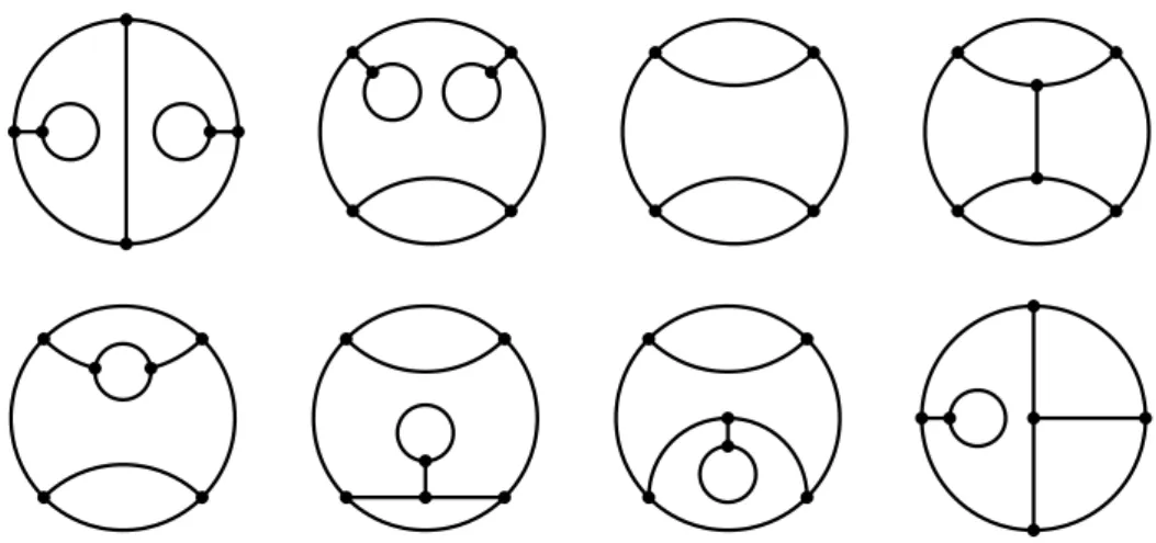
A skeleton satisfying these conditions is called generic. Note that any skeleton satisfying condition (1) is a bipartite graph. For this reason, in the drawings below we omit bivalent ◦-vertices, assuming that such a vertex is to be inserted in the middle of each edge connecting two •-vertices. In particular, for a generic skeleton, only singular monovalent ◦-vertices are drawn.
A region of a skeleton Sk ⊂ P1 is a connected component of the complement
P1r Sk. One can also speak about closed regions, which are connected components
of the manifold theoretical cut of P1 along Sk. (In general, a closed region ¯R is not the same as the closure of the corresponding open region R.) We say that a
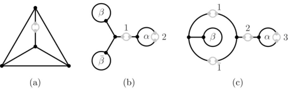
region R is an m-gon (or an m-gonal region) if the boundary of the corresponding closed region ¯R contains m •-vertices. For example, in Figure 4(b) below, the
three regions marked with α, β, and ¯β are monogons, whereas the outer region is a
nonagon. In Figure 4(c), there are two monogons (marked with α and β) and two pentagons.
Each region R of SkB contains a finite number of singular fibers of B, which can
be of one of the types 2.3(1)–(3) (excluding ˜A0, which is not singular). One can use
a sequence of inverse elementary transformations and convert these fibers to the ˜A type fibers starting the series. If R is an m-gonal region, the total multiplicity of these ˜A type fibers equals m.
2.6. Skeletons and maximal curves. The skeleton SkB of a maximal trigonal
curve B ⊂ Σk is necessarily generic and connected. (It follows that each region
of SkB is a topological disk.) Each m-gonal region R of SkB contains a single
singular fiber FR of B; its type is one of 2.3(2) if m = 1 or one of 2.3(3) with p = m if m > 2. Thus, the type of FR is determined by its multiplicity. The other singular fibers of B are over the singular vertices of SkB; the type of such a singular
fiber Fv is also determined by its multiplicity (and the type and the valency of v).
The function tsB sending each region R to the multiplicity mult FR and each
singular vertex v to the multiplicity mult Fv is called the type specification. It has
the following properties:
(1) tsB(m-gonal region R) = m + 6s, s ∈ Z>0;
(2) tsB(singular •-vertex v) = 2(valency of v) + 6s, s ∈ Z>0;
(3) tsB(singular ◦-vertex) = 3 + 6s, s ∈ Z>0;
(4) the sum of all values of tsB equals 12k.
The following statement is essentially contained in [10].
2.6.1. Theorem. The map B 7→ (SkB, tsB) establishes a bijection between the set
of isomorphism classes (equivalently, fiberwise equisingular deformation classes) of maximal trigonal curves in Σkand the set of orientation preserving diffeomorphism classes of pairs (Sk, ts), where Sk ⊂ S2 is a connected generic skeleton and ts is a function on the set of regions and singular vertices of Sk satisfying conditions
(1)–(4) above. ¤
2.6.2. Remark. Often it is more convenient to replace tsB with the Z>0-valued
function tdB sending each region and singular vertex to the integer s appearing
in (1)–(3). In term of tsB, the index k of the Hirzebruch surface Σk containing B
is given as follows, cf. [11]: #•+ #◦(1) + #•(2) = 2 ¡ k −PtdB ¢ ,
where #• is the total number of •-vertices, #∗(i) is the number of ∗-vertices of
valency i, andPtdB is the sum of all values of tdB. The singular points of B are
simple if and only if tdB takes values in {0, 1}; in this case,
P
tdB is merely the
number of triple singular points of B.
3. The Zariski–van Kampen method
In Subsections 3.1–3.3, we briefly remind the classical Zariski–van Kampen ap-proach [18] to the computation of the fundamental group of an algebraic curve and the construction of [8], which makes the braid monodromy of a genuine trigonal curve almost canonically defined. In Subsection 3.4, we introduce the concept of
slope which lets one treat a generalized trigonal curve in terms of its trigonal model
and, in particular, keep the braid monodromy B3-valued and easily computable. In
Subsections 3.5 and 3.6, we compute the local slopes and cite the results of [10] related to the global braid monodromy of a trigonal curve in terms of its skeleton. Finally, in Subsection 3.7, we consider a simple example, computing the groups of irreducible quintics.
3.1. Proper sections and braid monodromy. Fix a Hirzebruch surface Σk, k > 1, and a genuine trigonal curve B ⊂ Σk. The term ‘section’ below stands for a continuous section of (an appropriate restriction of) the fibration p : Σk→ P1.
3.1.1. Definition. Let ∆ ⊂ P1 be a closed (topological) disk. A partial section s : ∆ → Σk of p is called proper if its image is disjoint from both E and conv B.
The following statement is found in [8]; it is an immediate consequence of the fact that the restriction p : p−1(∆) r (E ∪ conv B) → ∆ is a locally trivial fibration
with connected fibers and contractible base.
3.1.2. Lemma. Any disk ∆ ⊂ P1 admits a proper section s : ∆ → Σk. Any two proper sections over ∆ are homotopic in the class of proper sections; furthermore, any homotopy over a fixed point b ∈ ∆ extends to a homotopy over ∆. ¤
Fix a disk ∆ ⊂ P1 and let b
1, . . . , br ∈ ∆ be all singular and, possibly, some
nonsingular fibers of B that belong to ∆. Denote Fi = p−1(bi). We assume that
all these fibers are in the interior of ∆. Denote ∆] = ∆ r {b
1, . . . , bl} and fix
a point b ∈ ∆]. The restriction p]: p−1(∆]) r (B ∪ E) → ∆] is a locally trivial
fibration with a typical fiber F◦
b r B, and any proper section s : ∆ → Σk restricts
to a section of p]. Hence, given a proper section s, one can define the group πF := π1(Fb◦r B, s(b)) and the braid monodromy m : π1(∆], b) → Aut πF. More
generally, given a path γ : [0, 1] → ∆] with γ(0) = b, one can define the translation homomorphism mγ: πF → π1(Fγ(1)◦ r B, s(b)).
Denote by ρb ∈ πF the ‘counterclockwise’ generator of the abelian subgroup
Z ∼= π1(Fb◦r conv B) ⊂ πF. (In other words, ρb is the class of a large circle in Fb◦
encompassing conv B ∩ F◦
b.) Since the fibration p−1(∆) r (conv B ∪ E) → ∆ is
trivial, hence 1-simple, ρb is invariant under the braid monodromy and is preserved
by the translation homomorphisms. Thus, there is a canonical identification of the elements ρb0, ρb00 in the fibers over any two points b0, b00∈ ∆]; for this reason, we
will omit the subscript b in the sequel.
In this paper, we reserve the terms ‘braid monodromy’ and ‘translation homo-morphism’ for the homomorphisms m constructed above using a proper section s. Under this convention, next lemma follows from Lemma 3.1.2 and the obvious fact that the braid monodromy is homotopy invariant.
3.1.3. Lemma. The braid monodromy m : π1(∆], b) → Aut πF is well defined and independent of the choice of a proper section over ∆ passing through s(b). Given a path γ in ∆], the translation homomorphism mγ is independent of the choice of a proper section passing through s(γ(0)) and s(γ(1)) up to conjugation by ρ. ¤
3.2. The Zariski–van Kampen theorem. Pick a basis {α1, α2, α3} for πF and
a basis {γ1, . . . , γr} for π1(∆], b). Both Fb◦ r B and ∆] are oriented punctured
planes, and we usually assume that the bases are standard: each basis element is represented by the loop formed by the counterclockwise boundary of a small disk centered at a puncture and a simple arc connecting this disk to the base point; all disks and arcs are disjoint except at the common base point. With a certain abuse of the language, we will refer to γi (respectively, αj) as the generator about the i-th
singular fiber (respectively, about the j-th branch) of B. We also assume that the basis elements are numbered so that α1α2α3= ρ and γ1. . . γr is freely homotopic
to the boundary ∂∆. Under this convention on the basis {α1, α2, α3}, the braid
monodromy does indeed take values in the braid group B3⊂ Aut πF.
Using a proper section s, we can identify each generator γiwith a certain element
of a section. The following presentation of the latter group is the essence of Zariski– van Kampen’s method for computing the fundamental group of a plane algebraic curve, see [18] for the proof and further details.
3.2.1. Theorem. In the notation above, one has
π1(p−1(∆]) r (B ∪ E), s(b)) = α1, α2, α3, γ1, . . . , γr ¯ ¯ γ−1 i αjγi= mi(αj), i = 1, . . . , r, j = 1, 2, 3 ® , where mi= m(γi), i = 1, . . . , r. ¤
3.3. The monodromy at infinity and relation at infinity. Let ∆ ⊂ P1 be a
disk as above. Connecting ∂∆ with the base point b by a path in ∆]and traversing it
in the counterclockwise direction (with respect to the canonical complex orientation of ∆), one obtains a certain element [∂∆] ∈ π1(∆], b) (which depends on the choice
of the path above). The following two statements are proved in [8].
3.3.1. Lemma. Assume that the interior of ∆ contains all singular fibers of B.
Then, for any α ∈ πF, one has m([∂∆])(α) = ρkαρ−k. In particular, the image
m([∂∆]) ∈ Aut πF does not depend on the choices in the definition of [∂∆]; it is called the monodromy at infinity. ¤
3.3.2. Lemma. Assume that the interior of ∆ contains all singular fibers of B.
Then a presentation for the group
π1(Σkr (B ∪ E ∪
Sr
i=1Fi), s(b))
is obtained from that given by Lemma 3.2.1 by adding the so called relation at
infinity γ1. . . γrρk= 1. ¤
It remains to remind that patching back in a singular fiber Firesults in an extra
relation γi= 1. Hence, for a genuine trigonal curve B, one has
(3.3.3) π1(Σkr (B ∪ E)) = α1, α2, α3 ¯ ¯ mi= id, i = 1, . . . , r, ρk = 1 ® ,
where each braid relation mi = id, i = 1, . . . , r, should be understood as a triple of
relations mi(αj) = αj, j = 1, 2, 3.
3.4. Slopes. Now, let ˜B ⊂ Σk˜be a generalized trigonal curve, and let B ⊂ Σk be
its trigonal model. Denote by F1, . . . , Frthe singular fibers of ˜B and let bi∈ P1 be
the projection of Fi, i = 1, . . . , r. The birational transformation between ˜B and B
establishes a diffeomorphism Σ˜kr ( ˜B ∪ E ∪ Sr i=1Fi) ∼= Σkr (B ∪ E ∪ Sr i=1Fi);
hence, it establishes an isomorphism of the fundamental groups. Let ˜Γi be a small
analytic disk in Σ˜kr E transversal to Fi and disjoint from ˜B and from the other
singular fibers of ˜B, and let Γi be the transform of ˜Γi in Σk. We will call Γi a geometric slope of ˜B at Fi. According to van Kampen’s theorem [18], patching back in the fiber Fi results in an extra relation [∂ ˜Γi] = 1 or, equivalently, [∂Γi] = 1.
Fix a proper (with respect to the genuine trigonal curve B) section s over a disk ∆ ⊂ P1 containing the projection p(Γ
F0
i = p−1(b0i) and γi0= [p(∂Γi)]. As above, we can regard γ0i both as an element of π1(∆], b0i) and, via s, as an element of π1(p−1(∆]) r (B ∪ E), s(b0i)). Furthermore,
we can assume that the basis element γi ⊂ π1(∆], b) introduced in Subsection 3.2
has the form γi = ζi· γi0· ζi−1, where ζi is a simple arc in ∆]connecting b to b0i.
Dragging the nonsingular fiber F0
i along γi0 and keeping two points in the image
of s and in Γi, one can define the relative braid monodromy
mreli ∈ Aut π1((Fi0)◦r B, Fi0∩ Γi, s(b0i)).
3.4.1. Definition. The local slope of a generalized trigonal curve ˜B at its singular
fiber Fiis the element κi0:= mreli (ξ)·ξ−1 ∈ π1((Fi0)◦rB, s(b0i)), where ξiis any path
in (F0
i)◦r B connecting s(b0i) and Fi0∩ Γi. The (global) slope of ˜B at Fi (defined
by a standard basis element γior, more precisely, by a path ζi connecting the base
point b to a point b0
i ‘close’ to bi) is the image κi:= m−1ζi (κ 0 i) ∈ πF.
The following two statements are immediate consequences of the definition. 3.4.2. Lemma. The slope κi is defined by the curve ˜B and generator γi up to conjugation by ρ (due to the indeterminacy of the translation homomorphism, see Lemma 3.1.3) and the transformation κi7→ mi(β)κiβ−1, β ∈ πF (due to the choice of path ξi in the definition). ¤
3.4.3. Lemma. In the fundamental group π1(p−1p(∂Γi) r (B ∪ E), s(b0i)), the conjugacy class containing [∂Γi] consists of all elements of the form γ0
iκi0, where κi0 is a local slope of ˜B at Fi. ¤
Note that, in view of Lemma 3.4.2 and the relation (γ0
i)−1βγi0 = m(γi0)(β), cf.
Lemma 3.2.1, the elements γ0
iκ0i do indeed form a conjugacy class.
As a consequence, in terms of the basis {α1, α2, α3, γ1, . . . , γr}, the relation
[∂Γi] = 1 resulting from patching the singular fiber Fi in the original surface Σ˜k
becomes γi = κi−1. Eliminating γi, the relations γi−1αjγi = mi(αj), j = 1, 2, 3, cf.
Lemma 3.2.1, turn into the braid relations (3.4.4) κiαjκ−1
i = mi(αj), j = 1, 2, 3, or m˜i= id,
where ˜mi: α 7→ κi−1mi(α)κi is the twisted braid monodromy.
Clearly, if Fi is a proper fiber, then Γi= ˜Γiand the path ξiin the definition can
be chosen so that κi= 1. In this case ˜mi= mi is still a braid.
3.4.5. Remark. In view of Lemma 3.4.2 and the fact that ρ is invariant under mi, for each fixed i = 1, . . . , r the normal subgroup of πF defined by the relations
˜
mi = id does not depend on the choice of a particular slope κi, and the projection
of κi to the quotient group πF/ ˜mi = id is a well defined element of this group
(depending on the curve ˜B and basis element γi only). In particular, each slope commutes with ρ (in the corresponding quotient), making irrelevant the ambiguity in the definition of the translation homomorphisms, see Lemma 3.1.3.
If all singular fibers are patched, hence all generators γi are eliminated, the
relation at infinity takes the form
(3.4.6) ρk = κ
r. . . κ1.
Finally, one obtains the following statement, cf. (3.3.3), expressing the fundamental group π1(Σ˜kr ( ˜B ∪ E)) in terms of the slopes and braid monodromy of the genuine
3.4.7. Corollary. For a generalized trigonal curve ˜B ⊂ Σ˜k one has π1(Σ˜kr ( ˜B ∪ E)) = α1, α2, α3 ¯ ¯ ˜mi= id, i = 1, . . . , r, ρk = κr. . . κ1 ® , where each braid relation ˜mi= id, i = 1, . . . , r, should be understood as a triple of relations ˜mi(αj) = αj, j = 1, 2, 3. ¤
The following statement simplifies the computation of the groups.
3.4.8. Proposition. In the presentation given by Corollary 3.4.7, one can omit (any) one of the braid relations ˜mi= id.
Proof. First, show that the first relation ˜m1 = id can be omitted. Each braid
relation ˜mi = id, i = 1, . . . , r, can be rewritten as κiα = mi(α)κi, α ∈ πF. Hence,
using all but the first braid relations, one can rewrite the relation at infinity (3.4.6) in the form ρk = ¯κ
1. . . ¯κr, where ¯κi= mr◦ . . . ◦ mi+1(κi) for i = 1, . . . , r − 1 and
¯
κr = κr. On the other hand, since mr◦ . . . ◦ m1 is the conjugation by ρ−k, see
Lemma 3.3.1, the product ˜mr◦ . . . ◦ ˜m1 is the conjugation by ρ−kκ¯1. . . ¯κr= 1. It
is the identity, and the relation ˜m1= id follows from ˜m2= . . . = ˜mr= id.
Now, assume that the relation to be omitted is ˜md = id for some d = 2, . . . , r.
Since ρ is invariant under m1, the relation ˜m1= id implies that κ1commutes with ρ.
Then, due to (3.4.6), it also commutes with κr. . . κ2 and (3.4.6) is equivalent to ρk = κ
1κr. . . κ2. Proceeding by induction and using only ˜m1= . . . = ˜md−1= id,
one can rewrite (3.4.6) in the form ρk = κ
d−1. . . κ1κr. . . κd, the right hand side
being a cyclic permutation of κr. . . κ1. On the other hand, the cyclic permutation {γd, . . . , γr, γ1, . . . , γd−1} is another standard basis for π1(∆], b), with the same
(but rearranged) slopes κi and braid monodromies mi, and with respect to this
new basis the braid relation to be omitted is the first one. Hence the statement follows from the first part of the proof. ¤
3.4.9. Remark. A by-product of the previous proof is the fact that, modulo (all but one) braid relations the slopes κr, . . . , κ1 cyclically commute, i.e., one has
κr. . . κ2κ1= κd−1. . . κ1κr. . . κd
for each d = 2, . . . , r. In particular, if there are only two nontrivial slopes (which is always the case in Section 5 below), their order in the relation at infinity (3.4.6) is irrelevant.
3.5. Local slopes and braid relations. Given two elements α, β of a group and a nonnegative integer m, introduce the notation
{α, β}m= (
(αβ)k(βα)−k, if m = 2k is even,
¡
(αβ)kα¢¡(βα)kβ¢−1, if m = 2k + 1 is odd.
The relation {α, β}m= 1 is equivalent to σm= id, where σ is the Artin generator
of the braid group B2 acting on the free group hα, βi. Hence,
(3.5.1) {α, β}m= {α, β}n= 1 is equivalent to {α, β}g.c.d.(m,n)= 1.
For the small values of m, the relation {α, β}m= 1 takes the following form:
– m = 0: tautology;
– m = 1: the identification α = β;
– m = 2: the commutativity relation [α, β] = 1; – m = 3: the braid relation αβα = βαβ.
Let Fi be a type ˜Ap (type ˜A∗0 if p = 0) singular fiber of a trigonal curve B, and
let bi = p(Fi) ⊂ ∆ be its projection. Pick a simple arc ζi: [0, 1] → ∆ connecting
the base point b to bi and such that ζi([0, 1)) ⊂ ∆]. We say that two consecutive
generators αj, αj+1 of πF, j = 1 or 2, collide at Fi (along ζi) if there is a Milnor
ball M about the point of non-transversal intersection of B and Fi such that, for
each sufficiently small ² > 0, the images of αj and αj+1under the translation along
the restriction ζi|[0,1−²]are represented by a pair of loops that differ only inside M ,
whereas the image of the third generator is represented by a loop totally outside M . In 3.5.2–3.5.4 below, we pick a standard basis {α1, α2, α3} for πF and assume
that two consecutive elements of this basis collide at Fi along a certain path ζi;
then we use this path ζi to construct a generator γi about Fi as in Subsection 3.2.
In other words, it is ζi that is used to define the global braid monodromy mi and
the slope κi. All computations are straightforward, using local normal forms of the
singularities involved; we merely state the results.
We denote by σ1, σ2 the Artin generators of the braid group B3 acting on the
free group πF = hα1, α2, α3i, so that σi: αi7→ αiαi+1α−1i , αi+17→ αi, i = 1, 2.
Note that the slope κi is only useful if the fiber Fi is to be patched back in (as
otherwise the presentation for the group π1(Σ˜kr ( ˜B ∪ E ∪ Fi∪ . . . )) would contain
the original generator γirather than κi). For this reason, after a small equisingular
deformation of ˜B + E, one can assume that ˜B is maximally transversal to Fi at
infinity. We do make this assumption below.
3.5.2. A proper fiber. Assume that Fi is a proper type ˜Ap (type ˜A∗0 if p = 0)
fiber of ˜B = B. Then one has:
(1) if α1 and α2 collide at Fi, then mi = σ1p+1 and κi = 1, so that the braid
relations are {α1, α2}p+1= 1;
(2) if α2 and α3 collide at Fi, then mi = σ2p+1 and κi = 1, so that the braid
relations are {α2, α3}p+1= 1.
3.5.3. A nonsingular branch at infinity. Assume that Fi is a type ˜Ap singular
fiber (type ˜A∗
0if p = 0 or no singularity if p = −1) and a single smooth branch of ˜B
intersects E at Fi∩ E with multiplicity q > 1. Then Fi is a type ˜Ap+2q singular
fiber of B and one has:
(1) if α1and α2collide at Fi, then mi= σ1p+2q+1and κi = (α1α2)q, so that the
braid relations are {α1, α2}p+1= [(α1α2)q, α3] = 1;
(2) if α2and α3collide at Fi, then mi= σ2p+2q+1and κi = (α2α3)q, so that the
braid relations are {α2, α3}p+1= [α1, (α2α3)q] = 1.
3.5.4. A double point at infinity. Assume that ˜B has a type Ap singular point at Fi∩ E and intersects E at this point with multiplicity 2q, 1 6 q 6 (p + 1)/2.
Then Fi is a type ˜Ap−2q singular fiber of B (with the same convention as in 3.5.3
for the values p − 2q = 0 or −1) and one has:
(1) if α1 and α2 collide at Fi, then mi = σ1p−2q+1 and κi = αq3, so that the
braid relations are σp−2q+11 (αj) = αq3αjα−q3 , j = 1, 2;
(2) if α2 and α3 collide at Fi, then mi = σ2p−2q+1 and κi = αq1, so that the
braid relations are σp−2q+12 (αj) = αq1αjα−q1 , j = 2, 3.
(If p − 2q = −1, there is no collision and mi= id. In this case, the slope is κi= αqj,
Now, assume that ˜B has a type A2p−1 singular point at Fi ∩ E and the two
branches at this point intersect E with multiplicities p and p + q for some q > 1. Then Fiis a type ˜A2q−1singular fiber of B, and one of the two branches of B at its
type A2q−1 singular point in Fi is distinguished: it is the transform of the proper
branch of ˜B. Choose generators α1, α2, α3 so that α1 and α2collide at Fi and α1
is the generator about the distinguished branch of B. Then
(3) mi = σ2q1 and κi = (α1α2)qαp1, so that the braid relations are [αp1, α2] = 1
and [(α1α2)qαp1, α3] = 1.
Finally, assume that ˜B has a type A2psingular point at Fi∩ E and intersects E
at this point with multiplicity 2p + 1. Then Fi is a type ˜A∗1 singular fiber of B
and, in an appropriate basis {α1, α2, α3}, such that α2 is the generator about the
branch of B transversal to Fi, one has
(4) mi= σ1σ2σ1and κi= α1αp+12 , so that the braid relations are [α1, αp+12 ] = 1
and α3= αp2α1α−p2 .
3.5.5. A triple point at infinity. Assume that ˜B has a triple point at Fi∩ E and
consider the (generalized) trigonal curve ˜B0 obtained from ˜B by one elementary
transformation centered at this point. Then the transform ˜Γ0
i of ˜Γi is still disjoint
from ˜B0 and thus can be used to define the slope of ˜B; hence the slope of ˜B at Fi
equals that of ˜B0. As a consequence, one has the following statement.
3.5.6. Corollary. For ˜B ⊂ Σk˜ and B00 ⊂ Σk+1˜ as above there is a canonical isomorphism π1(Σk˜r ( ˜B ∪ E)) = π1(Σ˜k+1r ( ˜B0∪ E)). ¤
3.6. Braid monodromy via skeletons. Let B ⊂ Σk be a trigonal curve, and
let Sk ⊂ P1 be its skeleton. Below, we cite a few results of [10] concerning the
braid monodromy of B in terms of Sk. For simplicity, we assume that all •-vertices of Sk are trivalent and all its ◦-vertices are bivalent (hence omitted). An alternative description, including more general skeletons, is found in [15].
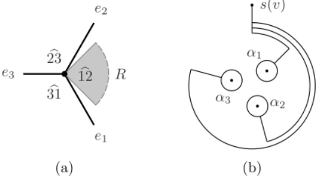
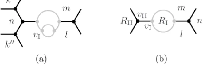
Recall that a marking at a trivalent •-vertex v of Sk is a counterclockwise order
e1, e2, e3of the three edges adjacent to v, see Figure 1(a). We consider the indices
defined modulo 3, so that ei+3 = ei. The three points of intersection of B and
the fiber Fv over v form an equilateral triangle. These points are in a canonical
one-to-one correspondence with the edges ei of Sk at v. Hence, a marking gives rise
to a canonical basis {α1, α2, α3} of the group πF = π1(Fv◦r B), see Figure 1(b);
this basis is well defined up to simultaneous conjugation by a power of ρ = α1α2α3.
e2 e1 e3 b 31 b 23 b 12 R s(v) α1 α2 α3 (a) (b)
As in Subsection 3.5, let σ1and σ2be the Artin generators of the braid group B3
acting on hα1, α2, α3i. Denote σ3= σ1−1σ2σ1 and extend indices to all integers via σi±3= σi. Note that the map (σi−1, σi) 7→ (σi, σi+1) is an automorphism of B3.
Recall also that the center of B3 is the cyclic subgroup generated by (σ1σ2)3 =
(σ2σ3)3= (σ3σ1)3.
3.6.1. The translation homomorphisms. Let u and v be two marked •-vertices
of Sk connected by a single edge e; to indicate the markings, we use the notation
e = [i, j], where i and j are the indices of e at u and v, respectively. Choosing a pair
of canonical bases defined by the markings, one can identify the groups π1(Fu◦r B)
and π1(Fv◦r B) with the ‘standard’ free group hα1, α2, α3i and thus regard the
translation homomorphism me: π1(Fu◦r B) → π1(Fv◦r B) as an automorphism of hα1, α2, α3i. It is a braid. However, since both the bases and the homomorphism me
itself are only defined up to conjugation by ρ (unless a proper section is fixed, see Lemma 3.1.3), this automorphism should be regarded as an element of the reduced braid group ¯B3= B3/(σ1σ2)3∼= PSL(2, Z). On the other hand, this ambiguity does
not affect the computation of the fundamental group, cf. Remark 3.4.5.
With the above convention, the translation homomorphism m[i,j]∈ ¯B3along an
edge e = [i, j] is given as follows:
m[i,i+1]= σi, m[i+1,i]= σ−1i , m[i,i]= σiσi−1σi, i ∈ Z.
The translation homomorphism mγ ∈ ¯B3 along a path γ composed by edges of Sk
is the composition of the contributions of single edges. If γ is a loop, the braid monodromy mγ is a well defined element of B3. It is uniquely recovered from its
projection to ¯B3just described and its degree (i.e., the image in B3/[B3, B3] = Z);
the latter is determined by the number and the types of the singular fibers of B encompassed by γ. More precisely, for a disk ∆ ⊂ P1 as in Subsection 3.1, the
composed homomorphism π1(∆]) → B3→ Z sends a generator γi about a singular
fiber Fi to the multiplicity mult Fi, see Subsection 2.2.
3.6.2. The braid relations resulting from a region. Given a trivalent •-vertex v
of Sk, one can define three (germs of) angles at v, which are represented by the connected components of the intersection of P1rSk and a regular neighborhood of v
in P1. If v is marked, we denote these angles b12, b23, and b31, according to the two
edges adjacent to an angle, see Figure 1(a). The position of a region R adjacent to v with respect to the marking at v can then be described by indicating the angle(s) that belong to R; for example, in Figure 1(a) one has b12 ⊂ R. Note that a region may contain two or even all three angles at v, see e.g. the outer nonagon and the central vertex in Figure 4(b) below.
Let ∆ ⊂ P1be a closed disk as in Subsection 3.1. Assume that v ∈ ∂∆ and that
∆ r v ⊂ R, cf. the shaded area in Figure 1(a). Then ∆ intersects exactly one of the three angles at v (in the figure this angle is b12). Take v = b for the base point and let {α1, α2, α3} be a canonical basis for πF = π1(Fv◦r B) defined by the marking
at v. The following three statements are straightforward; for details see [10]. 3.6.3. Lemma. If a disk ∆ as above intersects angle b12 (respectively, b23), then
α1and α2(respectively, α2 and α3) collide at any type ˜A singular fiber of B in ∆ along any path contained in ∆. ¤
3.6.4. Lemma. If a disk ∆ as above intersects angle b12 (respectively, b23 or b31),
the braid monodromy m : π1(∆], v) → Aut πF takes values in the abelian subgroup of B3 ⊂ Aut πF generated by the central element (σ1σ2)3 and σ1 (respectively, σ2 or σ3). If all singular fibers in ∆ are of type ˜A, then m takes values in the cyclic subgroup generated by σ1 (respectively, by σ2 or σ3). ¤
More precisely, in Lemma 3.6.4, the value of m on a type ˜Ap−1 fiber (type ˜A∗0if p = 1) is σip(assuming that ∆ intersects the angle spanned by eiand ei+1), and its
value on a type ˜Dq+4 fiber is (σ1σ2)3σqi. The value at a non-simple singular fiber
of type ˜Jr,pis (σ1σ2)3rσip.
3.6.5. Corollary. Assume that a region R of Sk adjacent to a marked vertex v
contains, among others, singular fibers of types ˜Api−1 ( ˜A∗0 if pi= 1), i = 1, . . . , s. Denote p = g.c.d.(pi). Then the braid relations mi= id resulting from these fibers are equivalent to a single relation as follows:
– {α1, α2}p= 1 if b12 ⊂ R;
– {α2, α3}p= 1 if b23 ⊂ R;
– {α1, α2α3α−12 }p= 1 if b31 ⊂ R.
In particular, if an m-gonal region R contains a single singular fiber, which is of type ˜A, it results in a single braid relation as above with p = m. ¤
3.6.6. Remark. In Corollary 3.6.5, if B is the trigonal model of a generalized trigonal curve ˜B ⊂ Σ˜k and it is π1(Σ˜kr ( ˜B ∪ E)) that is computed, one should
assume in addition that the fibers considered are proper for ˜B.
3.6.7. An irreducibility criterion. A marking of a skeleton Sk is a collection of
markings at all its trivalent •-vertices. A marking of a generic skeleton without singular •-vertices is called splitting if it satisfies the following three conditions:
(1) the types of all edges, cf. 3.6.1, are [1, 1], [2, 3], or [3, 2];
(2) an edge connecting a •-vertex v and a singular ◦-vertex has index 1 at v; (3) if a region R contains angle b12 or b31 at one of its vertices, the multiplicities
of all singular fibers inside R are even.
(Note that, given (1) and (2), the last condition holds automatically if R contains a single singular fiber, as R is necessarily a (2m)-gon.) The following criterion is essentially contained in [10]; it is obtained by reducing the braid monodromy to the symmetric group S3.
3.6.8. Theorem. A trigonal curve B ⊂ Σk with connected generic skeleton SkB is reducible if and only if SkB has no singular •-vertices and admits a splitting marking. Each such marking defines a component of B that is a section of Σk. ¤
3.6.9. Remark. A splitting marking defines a component of B as follows: over each •-vertex v, in a canonical basis {α1, α2, α3} defined by the marking, α1is the
generator about the distinguished component.
3.7. Example: irreducible quintics. As a simple example of application of the techniques developed in this section, we recompute the non-abelian fundamental groups of irreducible plane quintics, see [7] and [2]. A more advanced example is the contents of Section 5 below.
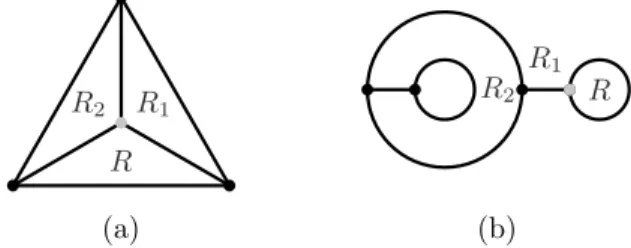
Let C ⊂ P2 be a quintic with the set of singularities A
6⊕ 3A2or 3A4. Blow up
trigonal curve ˜B ⊂ Σ1and let B ⊂ Σ2 be the trigonal model of ˜B. It is a maximal
trigonal curve with the combinatorial type of singular fibers 4 ˜A2 or 2 ˜A4⊕ 2 ˜A∗0; its
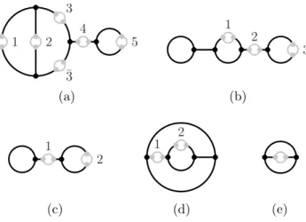
skeleton Sk is shown in Figures 2(a) and (b), respectively.
R R1 R2 R2 R1 R (a) (b)
Figure 2. Skeletons of plane quintics
Let R be the region of Sk containing the only improper fiber of ˜B. We choose for
the reference point b the vertex shown in the figures in grey and take for {α1, α2, α3}
a canonical basis over b defined by the marking such that b12 ⊂ R. In both cases, the only nontrivial slope κ = α3 is given by 3.5.4(1), with (p, q) = (4, 1) or (2, 1),
respectively. According to Proposition 3.4.8, the fundamental group
π1:= π1(P2r C) = π1(Σ1r ( ˜B ∪ E))
is defined by the relation at infinity and the braid relations resulting from three (out of four) regions R, R1, R2 shown in the figures. Using Subsection 3.6, one obtains
the following relations: for the set of singularities A6⊕ 3A2, see Figure 2(a): ρ2= α
3, {α2, α3}3= {α1, α2α3α−12 }3= 1,
(α1α2α1)α2(α1α2α1)−1= α3α1α3−1, (α1α2)α1(α1α2)−1= α3α2α−13 ,
and for the set of singularities 3A4, see Figure 2(b): ρ2= α
3, {α2, α3}5= {α2, ρ−1α1ρ}5, α1α2α−11 = α3α1α−13 , α1= α3α2α−13 .
In the former case, the group is known to be infinite, see [7], as it factors to infinite Coxeter’s group (2, 3, 7), see [6]. In the latter case, using GAP [17], one can see that
π1is a soluble group of order 320; one has
π1/π10 = Z5, π01/π100= (Z2)4, π001 = (Z2)2,
where0 stands for the commutant.
Certainly, this approach applies as well to other quintics with a double singular point. In particular, one can easily show that the groups of all other irreducible quintics are abelian.
4. Proof of Theorem 1.2.1
In Subsection 4.1, we replace a sextic as in the theorem with its trigonal model, which is a maximal trigonal curve in an appropriate Hirzebruch surface. Then, in Subsections 4.2 and 4.3, we enumerate the possible skeletons of trigonal models; in view of Theorem 2.6.1, this enumeration suffices to prove Theorem 1.2.1.
4.1. The trigonal models. Recall that, due to [11], an irreducible maximizing simple sextic cannot have a singular point of type D2k, k > 2 or more than one
singular point from the list A2k+1, k > 0, D2k+1, k > 2, or E7. Thus, a sextic as
in Theorem 1.2.1 has a unique type D point, which is either D5 or Dp with odd p > 7. We will consider the two cases separately.
Both Theorem 1.2.1 and Theorem 1.2.2 are proved by a reduction of sextics to trigonal curves. A key rˆole is played by the following two propositions.
4.1.1. Proposition. There is a natural bijection φ, invariant under equisingular
deformations, between Zariski open and dense in each equisingular stratum subsets of the following two sets:
(1) plane sextics C with a distinguished type Dp, p > 7, singular point P and without linear components through P , and
(2) trigonal curves B ⊂ Σ3 with a distinguished type ˜A1 singular fiber FI and a distinguished type ˜Ap−7 ( ˜A∗0 if p = 7) singular fiber FII6= FI.
A sextic C is irreducible if and only if so is B = φ(C), and C is maximizing if and only if B is maximal and stable.
4.1.2. Proposition. There is a natural bijection φ, invariant under equisingular
deformations, between Zariski open and dense in each equisingular stratum subsets of the following two sets:
(1) plane sextics C with a distinguished type D5singular point P and without linear components through P , and
(2) trigonal curves B ⊂ Σ4 with a distinguished type ˜A1 singular fiber FI and a distinguished type ˜A3 singular fiber FII.
A sextic C is irreducible if and only if so is B = φ(C), and C is maximizing if and only if B is maximal and stable.
The trigonal curve B = φ(C) corresponding to a sextic C via Propositions 4.1.1 and 4.1.2 is called the trigonal model of C.
Proof of Propositions 4.1.1 and 4.1.2. Let C ⊂ P2 and P be a pair as in the
statement. Blow P up and denote by ˜B ⊂ Σ1= P2(P ) the proper transform of C;
it is a generalized trigonal curve with two points at infinity. We let B = φ(C) to be the trigonal model of ˜B. The inverse transformation consists in the passage from B
back to ˜B ⊂ Σ1 and blowing down the exceptional section of Σ1.
The distinguished fibers FI and FII of B correspond to the two points of ˜B at
infinity (FI corresponding to the smooth branch of C at P ). It is straightforward
that, generically, the types of these fibers are as indicated in the statements. If the original sextic C is in a special position with respect to the pencil of lines through P , these fibers may degenerate: FI may degenerate to ˜A∗1 or ˜As, s > 1,
and FII may degenerate to ˜A∗∗0 (in Proposition 4.1.1 with p = 7) or to ˜As, s > 3
(in Proposition 4.1.2). However, using theory of trigonal curves (perturbations of dessins), one can easily see that any such curve B can be perturbed to a generic one, and this perturbation is followed by equisingular deformations of ˜B and C.
Since C and B are birational transforms of each other, they are either both reducible or both irreducible. The fact that maximizing sextics correspond to stable maximal trigonal curves follows from Theorem 2.4.2: for a generic sextic C as in the statements, one has µ(B) = µ(C) − 6 in Proposition 4.1.1 and µ(B) = µ(C) − 1 in Proposition 4.1.2. ¤
Let C be a sextic as in Theorem 1.2.1. Since C is irreducible, it has a unique type D point (see above), which we take for the distinguished point P . Denote by B ⊂ Σk, k = 3 or 4, the trigonal model of C and let Sk be the skeleton of B.
Let, further, RI and RII be the regions of Sk containing the distinguished singular
fibers FI and FII, respectively. Since we assume that C has no type E singular
points, B has no triple points (one has tdB ≡ 0, see Remark 2.6.2) and hence Sk
has exactly 2k •-vertices and has no singular vertices. Thus, due to Theorem 2.6.1, the proof of Theorem 1.2.1 reduces to the enumeration of 3-regular skeletons of irreducible curves with a prescribed number of vertices and with a pair (RI, RII) of
distinguished regions. This is done is Subsections 4.2 and 4.3 below.
4.2. The case Dp, p > 7. In this case, Sk has six •-vertices, RI is a bigon, and RIIis a (p − 6)-gon. Since p is not fixed, one can take for RIIany region of Sk other
than RI.
RI
RII RI
(a) (b)
Figure 3. A bigonal (a) and bibigonal (b) insertions
The bigonal region RI looks as shown in grey in Figure 3(a); we will call this
region the insertion. Removing RIfrom Sk and patching the two black edges in the
figure to a single edge results in a new 3-regular skeleton Sk0 with four •-vertices. Conversely, starting from Sk0 and placing an insertion at the middle of any of its edges produces a skeleton Sk with six •-vertices and a distinguished bigonal region, which we take for RI. Using Theorem 3.6.8, one can see that Sk is the skeleton of
an irreducible trigonal curve if and only if so is Sk0. There are three such skeletons (see e.g. [9]); they are listed in Figure 4. Starting from one of these skeletons and varying the position of the insertion (shown in grey and numbered in the figure) and the choice of the second distinguished region RII, all up to symmetries of the
skeleton, one obtains the 22 deformation families listed in Table 1. (Some rows of the table represent pairs of complex conjugate curves, see comments below.)
1 2 α β ¯ β 1 ¯ 1 2 3 α β (a) (b) (c)
Figure 4. A type Dpsingular point, p > 7
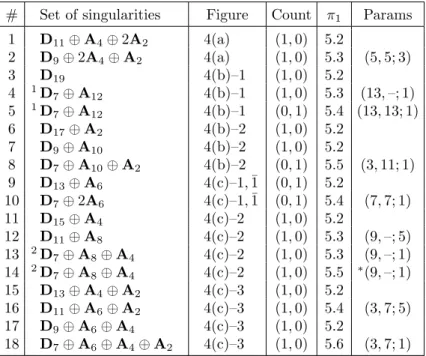
4.2.1. Comments to Tables 1 and 2. Listed in the tables are combinatorial types of singularities and references to the figures representing the corresponding skeletons. Equal superscripts precede combinatorial types shared by several items
in the tables. The ‘Count’ column lists the numbers (nr, nc) of real curves and pairs of complex conjugate curves, so that the total number of curves represented by a row is nr+ 2nc. The last two columns refer to the computation of the fundamental
group and indicate the parameters used in this computation. (A parameter list is marked with a∗when the general approach does not work quite well for a particular
curve. In this case, more details are found in the subsection referred to in the table.) Table 1. Maximal sets of singularities with a type Dp point, p > 7
# Set of singularities Figure Count π1 Params
1 D11⊕ A4⊕ 2A2 4(a) (1, 0) 5.2 2 D9⊕ 2A4⊕ A2 4(a) (1, 0) 5.3 (5, 5; 3) 3 D19 4(b)–1 (1, 0) 5.2 4 1D 7⊕ A12 4(b)–1 (1, 0) 5.3 (13, –; 1) 5 1D 7⊕ A12 4(b)–1 (0, 1) 5.4 (13, 13; 1) 6 D17⊕ A2 4(b)–2 (1, 0) 5.2 7 D9⊕ A10 4(b)–2 (1, 0) 5.2 8 D7⊕ A10⊕ A2 4(b)–2 (0, 1) 5.5 (3, 11; 1) 9 D13⊕ A6 4(c)–1, ¯1 (0, 1) 5.2 10 D7⊕ 2A6 4(c)–1, ¯1 (0, 1) 5.4 (7, 7; 1) 11 D15⊕ A4 4(c)–2 (1, 0) 5.2 12 D11⊕ A8 4(c)–2 (1, 0) 5.3 (9, –; 5) 13 2D 7⊕ A8⊕ A4 4(c)–2 (1, 0) 5.3 (9, –; 1) 14 2D 7⊕ A8⊕ A4 4(c)–2 (1, 0) 5.5 ∗(9, –; 1) 15 D13⊕ A4⊕ A2 4(c)–3 (1, 0) 5.2 16 D11⊕ A6⊕ A2 4(c)–3 (1, 0) 5.4 (3, 7; 5) 17 D9⊕ A6⊕ A4 4(c)–3 (1, 0) 5.2 18 D7⊕ A6⊕ A4⊕ A2 4(c)–3 (1, 0) 5.6 (3, 7; 1)
4.2.2. Remark. Items 4 and 5 in Table 1 differ by the choice of the monogonal region RII. We assume that nos. 4 and 5 correspond, respectively, to the regions
marked with α or β, ¯β in Figure 4(b). (In the latter case, the two choices differ
by an orientation reversing symmetry, i.e., the two curves are complex conjugate.) Similarly, we assume that nos. 13 and 14 in the table correspond, respectively, to the monogonal regions marked with α and β in Figure 4(c).
4.3. The case D5. In this case, Sk has eight •-vertices and two distinguished
regions, a bigon RI and a quadrilateral RII. If RI is adjacent to RII, then the
two regions form together an insertion shown in grey in Figure 3(b); we call this fragment a bibigon. As in the previous subsection, removing the insertion and patching together the two black edges, one obtains a 3-regular skeleton Sk0 with four •-vertices. The new skeleton Sk0 represents an irreducible curve if and only if so does Sk; hence, Sk0 is one of the three skeletons shown in Figure 4. Varying the
position of the insertion, one obtains items 19–26 in Table 2.
4.3.1. Remark. Unlike Subsection 4.2, this time the insertion has a certain orien-tation, which should be taken into account. For this reason, some positions shown in Figure 4 give rise to two rows in the table. Similarly, most positions shown in Figure 7 below give rise to two rows in Table 4.
![Table 4. Some reducible sextics with a type D 5 point Set of singularities Figure Params [π 1 , π 1 ]](https://thumb-eu.123doks.com/thumbv2/9libnet/5761438.116558/26.892.144.616.157.685/table-reducible-sextics-type-point-singularities-figure-params.webp)
