Optimal streaming of a single job in a two-stage flow shop

EUROPEAN JOURNAL OF OPERATIONAL

RESEARCH

ELSEVIER

European Journal of Operational Research 110 (1998) 42-62

Theory and Methodology

Optimal streaming of a single job in a two-stage flow shop

Alper $en ‘, Engin Topaloglu, omer S. Benli *

Department of’ Industrial Engineering, BiNcent University, 06533 Ankara, Turkey

Received 1 February 1995; accepted 1 March 1997

Abstract

Lot streaming is moving some portion of a process batch ahead to begin a downstream operation. The problem to be considered in this paper is the following: a single job consisting of U units is to be processed on two machines in the given order. Given a fixed number of possible transfer batches between the two machines, the problem is to find the timing and the size of the transfer batches (or, sublots) so as to optimize a given criterion. The schedules can be eval- uated based on job completion, sublot completion, or item completion times. In the single job lot streaming problem, minimizing job completion time corresponds to minimizing the makespan, for which formulas for optimal sublot sizes are available. In this paper, the results for the sublot and item completion time models are presented. 0 1998 Elsevier Science B.V. All rights reserved.

Keywords: Production; Scheduling theory; Lot streaming; Flow shops

1. Introduction

Lot streaming is moving some portion of a process batch ahead to begin a downstream operation al- lowing for the downstream operation to start earlier and hence improving the given criterion. Since the initial papers of Baker [l] and Trietsch [2], there has been considerable interest in the area. For a review of the literature, the reader is referred to [3,4]. In addition to its implications in Group Technology (leading to cell based manufacturing, resulting in shorter lead times and reduced work in progress inventories), Just- in-Time Systems (lot size of one) and OPT/Synchronous Manufacturing (transfer us. process batches), fu- ture significance of lot streaming techniques may possibly lie in the integration of production planning and machine scheduling. One problem with production planning models is that the sequencing require- ments on the resources cannot be easily accommodated, whereas machine scheduling models cannot expli- citly handle lot sizing.

* Corresponding author. E-mail: benli@bilkent.edu.tr ’ Currently at University of Southern California.

0377-2217/98/$19.00 0 1998 Elsevier Science B.V. All rights reserved. PIISO377-2217(98)00203-8

A. $en et al. I European Journal of Operational Research II0 (1998) 4242 43

In lot streaming it is assumed that a number ofjobs each consisting of a number of identical parts (or, items) are to be processed on a sequence of machines. In traditional machine scheduling models the items are available to be moved to the next machine only when UN items in the job complete processing on the current machine. If it is feasible to partition the job into sublots and transport each sublot to the next op- eration independent of other sublots, then the rate at which the parts reach the last machine increases, re- sulting in improved completion time of the parts in the last machine. As pointed out by Potts and Van Wassenhove [5].

Most scheduling models assume that no shipment is possible until the entire job is completed. How- ever, in this case, the customer may be out of stock while awaiting delivery. Assume, for example, that a customer has a low inventory of some product and places a replenishment order consisting of a num- ber of pallets to cover expected demand for the next few months. It may take several weeks to process the complete order. However, the customer service is improved, firstly by producing a few pallets in the near future to cover the customer’s demand during the month, and then by satisfying the remaining part of the order at some later date. It is now apparent that if items or sublots may be shipped imme- diately upon completion, decomposing a job into sublots may improve customer service.

An important feature of modeling lot streaming problems is the time when the parts in the last machine become u&able to be shipped to an (external or internal) customer. In their review of batching and lot-siz- ing literature, Potts and van Wassenhove [5] proposed three models:

Job completion time model. The shipment to the customer can take place only when all the parts in the job complete processing in the last machine.

Sublot completion time model. Each sublot can be shipped to the customer independently. The shipment to the customer takes place when all the parts in sublot complete processing in the last machine.

Item completion time model. Each part can be shipped to the customer whenever it completes processing in the last machine.

For each scheduling problem, the technology of the shop dictates whether or not lot streaming is al- lowed; and, if it is allowed, which of the above three type of models is appropriate for the problem. In all of the above models the sublots are available to be moved to the next machine, as soon as they are com- pleted in the current machine. The models differ primarily as to when the items in the last machine become available to be moved to the “customer”. In some cases, although the order is transported in sublots within the factory, it is delivered to the customer as a whole. This situation is depicted in the job completion time model. In other cases, the order may be shipped to the customer in batches (sublots), as in the sublot com- pletion time models. Customer service may further be improved if each unit is shipped to the customer in- dividually as soon as its processing is completed in the last machine. This situation can be represented by an item completion time model. All other things being equal, the optimal solution to the item completion time model gives the shortest average time that a unit stays in the work-in-process inventory and the maximum customer service. Thus, lot streaming, in addition to improving customer service, reduces the average work- in-process inventory in the shop.

This paper deals with optimal streaming a single job in two machine (flow) shop. Although there may be actual problems with these exact structures in which optimal solutions are desirable, the main motivation for this study was to investigate the analytical and computational problems in designing optimizing algo- rithms for the simplest non-trivial case. The results obtained can be used as building blocks and provide insights in designing algorithms for more complex shop structures, and provide bounds on the heuristic ap- proaches.

The next section defines the problem and presents a review of previous work in this area. In the follow- ing section, results are presented for sublot completion time model. Details of the proofs are given in Ap- pendix A. The final section summarizes the insights gained in this analysis.

44 A. ,Yen et al. I European Journal of Operational Research 110 (1998) 4262

2. The problem

The problem to be considered in this paper is the following: a single job consisting of U units is to be

processed on two machines. Let pi,

i =

1,2, be the processing time of each unit on machine i. There are s

sublots on each machine. In this study, we shall assume that the sublots are consistent. That is, the sublots

are same size at each machine. Lk, k = 1,

. . . ,s

is the size of (i.e. the number of units in) the kth sublot,

c;=, Lk = u. F ur th ermore, the analysis in this paper will be based on allowing for fractional number of

units in a sublot. If the job contains large number of units, then this is an acceptable assumption. On

the other hand, if the number of units in the job is such that the fractional sublot sizes are not meaningful,

then one has to impose the integrality requirement on the sublot sizes (Lk > 0, and integer), resulting in a

mixed-integer program. C& is the completion time of kth sublot on machine i. The problem is to find the

timing and the size of the sublots on each stage so as to minimize a given optimality criterion.

Under these assumptions, the problem can be described by the following constraints.

Cik>Ci,k_l$piLk,

i=l,2,

k=l,...,s,

C2k 3 Clk +p2Lk,

k= l,...,s,

s

c

Lk =

u,

k=l CiO = 0,

i= 1,2,

₍₄₎

c,k 2 0, i=

1,2,

k= l,...,~,

(5)

Lk 3 0,

k= l,...,~.

₍₆₎

Constraints (1) allow sublot k to start only after sublot k - 1 is completed. Constraints (2) prevent a sub-

lot to be processed simultaneously on both machines. Constraint (3) assures the sublots to account for all

the units in the job.

Various performance criteria can be used with these constraints. For example, in the job completion time

model, defined earlier, the objective function is minimizing CzS subject to Constraints (l)-(6). Note that

there is no distinction between makespan and total flowtime when there is one job in the problem. In other

words, minimizing total flowtime corresponds to minimizing makespan, or CzS_

The m-machine version of

this problem was first studied, independently, by Baker [l] and Trietsch [2]. Baker [l] gave the linear pro-

gramming formulation of the problem. Baker [l] and Potts and Baker [6] showed that for two-machine case,

the closed form solution is given by the geometric sublot sizes

l-7t

L1=U----

1 - rcs’

Lk = dk_1,

k=2,...,s,

₍₈₎

where rc 3

pz/pl

If one uses equal sublot sizes, which are more convenient in practice, Potts and Baker [6]

have shown that, FE(L)/F* (L) < 1.09, where F*(L) is the optimal job completion time when geometric sub-

lot sizes are used and FE(L) is the job completion time when equal sublot sizes are used.

In sublot completion time model an item leaves the shop when the sublot to which it belongs is com-

pleted in the second machine. Total flowtime of all units in the job is Cbl Lk&. Minimizing total flowtime

is equivalent

to minimizing the average time a unit spends in the shop, i.e. the mean flowtime,

(l/U) c”,=, LkC2k. Note that, this is not “weighted” mean flowtime in the traditional sense, since Lk’s

cannot be exogenously assigned, but are endogenous variables of the problem. The problem becomes a

A. $en et al. I European Journal of Operational Research 110 (1998) 4242 45

quadratic programming problem with the objective function minimizing C;I=, LkC2k subject to Constraints (l)-(6). This model is analyzed further in Section 3.

Finally, in the item completion time model an item is assumed to be completed as soon as it completes processing in the last machine. When continuous sublot sizes are allowed, this is equivalent to assuming “infinite” number of transfers in the last machine (in other words, after the first sublot starts in the second machine, parts in the second machine become available to be shipped to a customer “continuously”). In the case of two-machine flow shop with consistent sublot sizes, the objective function is min Ci=,[C’2k- 032/2)Lk]Lk subject to Constraints (l)-(6). There are two cases to consider: (i) n d 1, and (ii) 7~ > 1 where rt z n/pi. Cetinkaya and Gupta [7] have shown if rt < 1, then equal size sublots are optimal, otherwise one has to use the geometric sublot sizes given in Eqs. (7) and (8). Again, as in the case of job completion mod- el, it may be more convenient to use equal size sublots in practice, even when 71 > 1. For notational con- venience, let U = 1. pl = 1, and p2 = rc, and denote by F*(L) the optimal mean item completion time when geometric sublot sizes are used, and FE(L) be the mean item completion time when equal sublot sizes are used. It can be observed in Figs. 1 and 2, that FE(L) = l/s + irt, and F*(L) = (7~ - l)/(r’ - 1) + +rc. It can be shown, using similar computations as in Section 3.2, that FE(L)/F*(L) < 1.18. (Numerical solutions in- dicate the largest value for the ratio to be 1.172 at s = 4 and 7~ = 2.021.)

3. The sublot completion time model

The model to be discussed in this section is the sublot completion model of streaming a single job in a two-machine shop. In this model, each sublot can be shipped to the customer independently. The shipment to the customer takes place when all the parts in sublot complete processing in the second machine. The problem is a quadratic programming problem with the objective function

Average Delivery Time Fig. 1. Item completion, equal sublot sizes

I I I I I---

l I I

llllllllllJllllllllllllll~l~~lllllllllllllll~lllllllllll~~

I%\-

A

Average Delivery Time Fig. 2. Item completion, optimal sublot sizes.

46 A. Fen et al. I European Journal of Operational Research 110 (1998) 4242

LkC2k k=l

subject to Constraints (l)-(6).

This quadratic objective function was first proposed by Kropp and Smunt [8]. When the sublots are as-

sumed to be consistent, they gave a complete formulation for m-machine problem using the linear con-

straints proposed by Baker in [l]. When there are only two sublots allowed between the machines, i.e.,

s = 2, efficient algorithms are proposed by Cetinkaya and Gupta [7] and Topaloglu et al. [9].

For the two-machine problem, letting rc = pz/pi, we have the following two results:

Result 1. If 71 d

1,

then the sublots of equal size are optimal, i.e.

L; = u/s, k=

l,...,s.

₍₁₀₎

Result 2. If 71 >

1

optimal sublots can be found by the following algorithm.

Algorithm 1

u t 0,

optimal t FALSE

If f (77) = -7+ + 2ti+’ + 2n” - 27t-

1 > 0

optimal t TRUE, geometric sublots are optimal

While not

optimal

vtu+l

Z1 t U[Y7t

- (s - ~)]/[$=+(S

- u) + ($=$‘7r]

zk c~~-~z,, k=2 ,..., v

~kt[U-E1C1;=l~‘-‘]/[(S-U)], k=V+l,...,s if 7x t, 3 Ev+l 3 I,,

optimal t TRUE, z = Et,.

. . , Es)

is optimal

Basically, the above algorithm creates geometric sublot sizes (with ratio rc) up to sublot u, followed by

equal sublot sizes for the rest of the schedule. The algorithm then checks a necessary condition to see if the

current value of u is optimal; if not, it looks for a better choice of u. The search starts at u = 1 and stops as

soon as the necessary condition is satisfied.

Result 1 is due to Cetinkaya and Gupta [7]; an alternate proof is given in Section A. 1. Result 2 was con-

jectured but not proven in Cetinkaya and Gupta [7]; a detailed proof of this result is given in Section A.2.

It is difficult to give an intuitive explanation for the resulting sublot sizes obtained by the above algo-

rithm. It is not possible to have a general closed form solution for the sublot sizes. For certain values of

s, though, closed form solutions can be obtained. For example, for s = 2 and s = 3, optimal sublot sizes

are given below.

Solution for s = 2

(

__.L_n

@T,LZ) =

{

X+l’rr+l

>

if 1<7c<l+Jz,

(

*,+

n >

if l+fi<n.

(11)

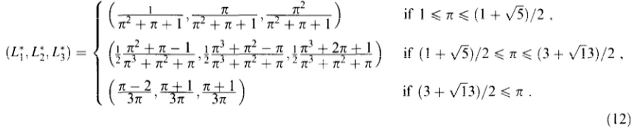
Solution for s = 3

A. $en et al. I European Journal of Operutional Research 110 (1998) 42-62 47 ( I 72 7c2+7[+1~7c2+~+1h2+71+1 > if 1 < 7r d (1 + fi)/2 , ( $+a-1 17c3+7c-n 1n3+27c+l -~r’+712+n’27C3+T12+71’2713+712+7C > if (1 + &)/2 6 7~ d (3 + &3)/2 , if (3 + Ji3)/2 d n . (12)

3.1. Variable size sublots

The above results for sublot completion time model are based on the requirement that sublots are con- sistent, i.e. the size of the kth sublot is Lk in both of the machines. Suppose we relax this requirement, and thus define variable size sublots as Lik, i = 1, . . , s to be the number of units in the kth sublot on machine i. One would expect an improvement in the objective function value when sublot sizes are allowed to vary. Feasible solutions with consistent sublot sizes constitute a proper subset of the set of feasible solutions with variable size sublots; therefore, the optimal solution with variable size sublots must be at least as good as the optimal solution with consistent sublot sizes. In the two-machine job completion time model, as pointed out by Trietsch and Baker [3], this relaxation will not improve on the optimal solution with consistent sub- lot sizes, since there is only one set of transfers between the machines ~ from the first machine to the second. In job completion time model, there is only one transfer from the second machine: items become available to be shipped to the customer only when last sublot is completed in the second machine.

This is not necessarily the case in the two-machine sublot completion time models, as the following ex- ample illustrates. Suppose that a job consisting of 60 units is to be processed in a two-machine flow shop using at most two sublots. Let the processing times be p1 = 1 and p2 = 3. With s = 2 and 71 = 3, from ex- pression (1 l), (LT, L;) = (20,40); resulting in a mean sublot completion time (a mean flowtime) of &,(20 x 80 + 40 x 200) = 160. But a better mean sublot completion time of &30 x 105 + 30 x 195) =

150 can be achieved using (L;, , LT2) = (15,45) and (Lz, , LG2) = (30,30) (see Fig. 3). This leads us to consider the following conjectures:

Ml I 1

M2

20 60 80

Optimal Consistent Sublot Sizes

Ml M2

200

Mean ELow Time = 160

I

15 60 105 195

Variable Sublot Sizes Mean Flow Time = 150

48 A. Sen et al. I European Journal of Operational Research 110 (1998) 42-62

Conjecture 1.

Mean sublot completion time is minimized by equal sublots on each stage

if pi

>, ~2.

Conjecture 2.

Mean sublot completion time is minimized by geometric sublots on first stage, and equal sub-

lots on second stage if pi < ~2.

The following intuitive justification can be provided for these conjectures:

processing should be continu- ous on the dominant machine and start as early as possible.

For

p1 3 pz,

the first machine is dominant and

determines the sublot sizes. For

p1 < p2,

the dominant machine is the second one and geometric sublots on

the first machine allow the second machine to start continuous production as early as possible.

3.2.

Equal size sublots

If pI 3 ~2,

then equal size sublots are optimal for the problem with consistent sublot sizes. (If Conjecture

1 is true, then equal size sublots are optimal even when

oariable

size sublots are allowed.) As with the other

models, for practical reasons, one may choose to use equal size sublots also in the case when

p1 < pz.

It will

be useful to determine how much impairment this approximation will cause in the mean sublot completion

time. For notational convenience, let U = 1,

p1 =

1, and pz = rc; when

p1 < p2,

i.e. n > 1, mean sublot

completion time with equal sublot sizes (see Fig. 4) is

FE(L) =

(s y),

‘+ !

‘+

(;+~~)~+...+(f+7c~)~

(s+ 1)

=$+s-

2s (13)

Since it is not possible to derive explicit expression for the optimal mean sublot completion time using

consistent sublots, Fe(L), we shall use a lower bound for its value. We know (from Result 7 in Appendix A)

that,

XLk 3 Lk+lr k=

l,...,s-

1

is a necessary condition for optimality.

Consider the following linear program:

z = minLi

subject to

XLk 2 Lk+l> k=

l,...,s-

1,

s

c

Lk = 1, _{Lk>o, k=l,..., s-l.}

k=l

It is not difficult to show that z = (rc - l)/(rc” - 1). Thus, the smallest possible size of the first sublot on

the first machine is z. Since

p1 =

1, z is the earliest time the second machine can start processing. Once the

second machine starts processing, it will continue uninterrupted

because 7~ > 1 and the first constraint,

XLk > Lk+i,

k =

1,.

. . ,s -

1. Thus a lower bound for the optimal sublot completion time, F’(L), is given

by the minimal value of the following quadratic program:

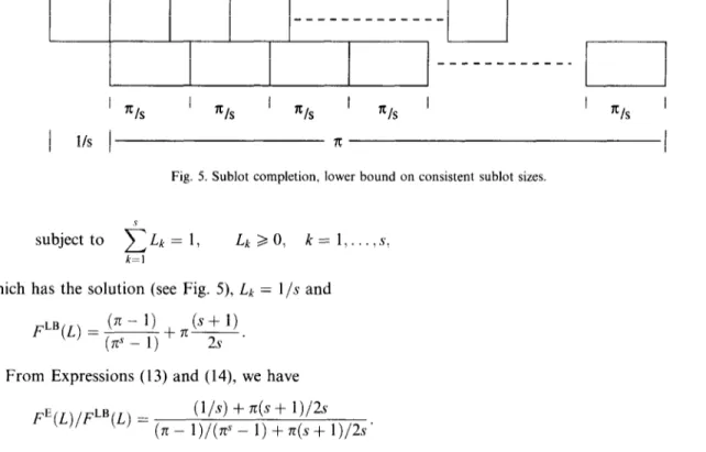
A. $en et al. I European Journal of Operational Reseurch I10 (1998) 42 62 49

Fig. 5. Sublot completion, lower bound on consistent sublot sizes.

subject to

2~~

=

1, Lk 20, k=

l,...,s.

k=l

which has the solution (see Fig. 5),

Lk =

l/s and

(n-

1)

FLB(L) = (@ _ 1) + n

(s+

_2s

1)

_. (14)

From Expressions (13) and (14), we have

P(L)/P(L) =

(l/s) + rc(s + 1)/2s

(7t - l)/(rc” - 1) + 7c(s + 1)/2s’

Suppose s can take any real value, then f(rr, s) = FE(L)/FLB(L)

. IS

a continuous function of s and 7~ for

s 3 2 and 7c > 1. Setting the partial derivatives of f(n,s) with respect to s and 71 equal to zero, and solving

the resulting two non-linear equations numerically, gives a unique solution

(rc’, s*) =

(1.938,4.267). (Since

[a2f(~*,s*)/i)7lns]2-(32f(s*,g’)/aa)(B2~(~*,~*)/&2)

= -0.00184, (n*,s*) is a maximum point.)

Clearly,

for discrete

values of s, the maximum

of f(rc, s) should be less than f(lc*, s*) =

.f( 1.938.4.267) = 1.14. For example, f(%, s^) = f( 1.992,4) = 1.139. Thus, we have the following result.

Result 3.

FE(L)/FLB(L) <

1.14.

Since FLB(L) d F’(L), FE(L)/FC(L) d

FE(L)/FLB(L),

thus by Result 3,

FE(L)/FC(L) <

1.14.

It is interesting to observe that the sublot sizes found while constructing a lower bound for the model

with consistent sublot sizes are “geometric sublot sizes in the first machine” and “equal size sublot sizes

r-_rr

____________

m

’

X/s

I n/S I AIS I B/S I I =lS I

I-

;s::

-

7T

T

50 A. ,Ten et al. I European Journal of Operationul Research 110 (1998) 4242

in the second machine”;

which is the claim in Conjecture

2. If this conjecture

is true, then

FE(L)/F’*(L) < 1.14, where

F*(L)

is the mean sublot completion time achievable by allowing for variable

size sublots.

4.

Conclusions

In this paper we have analyzed lot streaming of a single job in a two-stage flow shop. Where applicable,

the distinction between the consistent and variable size sublots were emphasized. The implications of equal

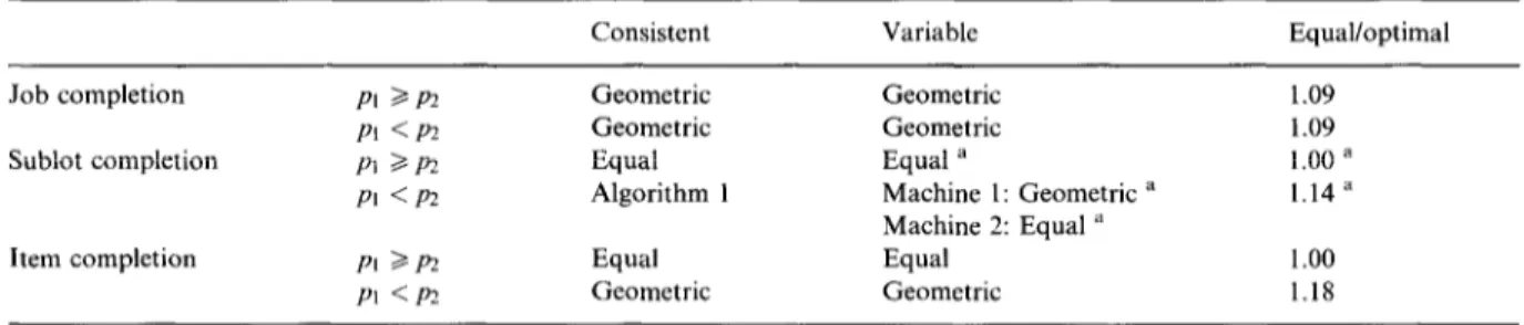
sublots, which are widely used in practice were also presented. Table 1 summarizes the results. (In the item

completion time model, the sublot sizes to be determined are between the first and the second machines,

since the items leave the second machine one at a time as they are completed; therefore, the distinction be-

tween consistent and variable size sublots in this model is not relevant.)

Even when variable sublot sizes are allowed, consistent sublots are optimal in all cases, except in sublot

completion time model with pi <

~2.

As seen from the last column of Table 1, equal sublots are quite ef-

fective, justifying the use of equal sublots in practice.

Acknowledgement

Authors would like to thank the anonymous referee for relevant and helpful comments that have greatly

improved the paper.

Appendix A

In this appendix detailed proofs of the results obtained in sublot completion time model are presented.

Result 1 is due to Cetinkaya and Gupta [7]. An alternate proof is given below. Then it is shown that the

algorithm in Result 2 finds the optimal solution.

A.1. Result 1

If p2/p1 s rc <

1,

then the sublots of equal size are optimal for the sublot completion time, i.e.

L; = U/s, k=

l,..., s.

Table 1 Sublot sizes

Consistent Variable Equal/optimal

Job completion Sublot completion Item completion PI aP2 PI <P2 PI >P? PI <P2 PI aP2 PI <pz Geometric Geometric Equal Algorithm 1 Equal Geometric Geometric Geometric Equal a Machine 1: Geometric a Machine 2: Equal ” Equal Geometric 1.09 1.09 1.00 a 1.14 a 1.00 1.18 a Conjectured.

A. $en et al. I European Journal of Operational Research I10 (I 998) 42 d2 51

Proof. Consider the general case: there are m machines, with the property pI > max2 4 i G m(pj}, and we will show that equal sublot sizes (i.e. Lk = U/s, k = 1, . . . ,s) are optimal. Without loss of generality, assume that U = 1, then we have the following formulation for an m-machine flow shop.

min F(L) = C~_iLkCmk subject to x’L=,Lk = 1 , CII -plLl 30 , Cjk-Cj,k_-] -piLk 20, i= I,..., m, k=2 !.... s, cik - C;-l,k -piLk > 0, i= l,...,m, k = 2, . . 1 s, Cik 2 0, i= l,...,m, k=2,....s, Lk 3 0, k= l,...,~.

We first need the following result showing that there exists an optimal solution with non-decreasing sub- lot sizes.

Result 4. Zf p1 2 max2 G i 4 ,(pi} then an optimal solution exists in which,

Lk <Lk+l, k= l,...,s. ₍₁₅₎

Proof. Suppose the contrary, that is, there exists an optimal solution L = (LI , . . , L,) such that for at least

One k, Lk > L&l.

Now we will give an algorithm that will construct a schedule satisfying Condition (15) and having the objective value not more than that of L. Let II, = (II,(l), I&(2), . , II,(s)) and n = (II(l), II(2), ~ ii(s)) denote the sublot sequence at tth i .teration of the algorithm and the optimal sublot sequence, respectively. no + i=I for t = 0 to s - 1 do begin r + argmax{ 1 G k G s-t}{LIX,(k)) n /+1 + n, for k = r to s - t do I&+1(k) + n4k-t 1) l-L,l(S - 4 + l-l&) end

In the tth iteration of first for loop, the minimum sublot among the first (s - t) sublots in the sequence II, is removed from its place and inserted in (s - t)th place to form the sequence I’&+l. The final schedule satisfies

To show that the resulting schedule has objective value not more than the optimal solution, consider the following two observations:

Result 5. In the tth iteration of the algorithm, if the largest sublot among the first (s - t) sublots, n,(r), is removedfrom the schedule, then the minimum decrease in the totalflowtime A- is

52 A. $en et al. I European Journal of Operational Research 110 (1998) 4262

A-

2

PI&I,(,)

2

&(I).

I=r+l

Proof.

Let CP be the minimum decrease in the completion time of the sublots that follow the removed sub-

lot. Clearly,

A- 2 C- c LrI,(l)~

l=r+l

As illustrated in Fig. 6, a lower bound on the C can be found as

The lot streaming problem turns out to be an ordered flow shop problem, when the sublot sizes are gi-

ven. This result follows from two facts. First, if a sublot has the kth largest processing time on machine i,

then it has the kth largest processing time on every other machine. Second, if a sublot has its ith largest

processing time on machine e, then every other sublot has the ith largest processing time on machine e.

In ordered flow shops, when the first machine has the largest processing time, the minimum makespan is

achieved, if the jobs are in non-increasing order of processing times. This result is given in Smith et al.

[lo].

In order to prove this result, they consider an optimal sequence with at least one job whose processing

time is larger than the processing time of the immediately succeeding job. They show that, the new sequence

formed by pairwise interchange of these two jobs does not have a longer makespan. This implies, however,

that the longest makespan is achieved when the jobs are in non-decreasing order of processing times. Using

this fact, we get

Sublot lI, (r)

Ml

M2

M3

. . .

M4

A. ,Ten et al. I European Journal of Operational Research I10 (1998) 42-62 53

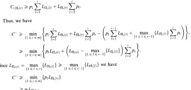
The expression on the right is the maximum completion time that can be achieved on the ith machine by

sequencing the first r -

1

sublots. The following is a lower bound on Ci,n,(r):

Thus, we have

2

PIhI,(

Hence, the minimum decrease in the objective function is

.,...__...__...._...

. . ..*....*...

*...__...__...**

54 A. Sen et al. I European Journal of Operational Research 110 (1998) 42-62

s

A-

2

PI&(~)

c

h,(r).

0

I=r+l

Result 6. If

the largest sublot among the first t sublots, II,(r), is inserted (s - t) th place in the schedule

(Fig. 7), then the maximum increase in the totalflowtime

Ai is

A+

G P&I,(~) 2

LrL(l)~

I=r+l

Proof. Let C+ be the increase in the completion time of removed sublot, when it is inserted in the (s - t)th place. Observe that

A+ = Ln,(r)C+

+

PI&I,(,) 2

Lrq[)

I?-t+l C+ can be written as s-t ’ p1 CL%(l) + Lnt(r) 2

Pv -

Pl

2

k,(l) +

Ln,(,) gp”

I=1 v=2 ( I=1 u=2 )

s-t d Pl c Ln,(r).

I=r+ I

Hence, the maximum increase is

s-t s

A+

d

prLrqY) C h(r) + PILrql) C h,(l)

l=r+l I=s-ffl

G PlLn,(r) 2 h,(l). 0

l=r+l

Therefore, in the tth step of proposed algorithm, the maximum overall increase in the mean flowtime value is

A+ - A- < 0.

Hence, the mean flowtime of the sublot schedule constructed by the algorithm is not worse. Thus, in the optimal solution, Lk 6 &+I, k = 1,. . . ,S.

As shown in Fig. 7, the completion time of the sublot

k

on the last machine is,

k-l

&k =Pl CL, +&pi.

I=1 i=l

With this property the following concise formulation with a convex objective function and fewer con- straints can be obtained;

A. $en et al. I European Journal of Operational Research I10 (1998) 4262 55 min Lkcmk k=l k-l S.t. Cmk -PI C Ll - Lk epi = 0, k= l,...,s. /=I i=l 2 Lk = 1 k=l or, equivalently, min -b + Lk .&i i=l s s.t. c Lk= 1. k=l

Proof (Result 4). The Lagrangian function of the above problem is

then 89 ~=p1~L1+2L~~pi-p~L,+6=0 I=1 i=l and dY

s

x=c

L,-l=O. r=l Since

--_=

=r

a+1

2(Lr - Lr+l) ppi _i=l -plLr +plLr+l = 0 or

Lr(2gPi-Pl) =L,ilj2gPi-pl),

But ci=, Lk = 1 implies that L, = l/s is the candidate optimal solution. However, to prove that it is the desired solution, we have to show that the objective function is convex. The Hessian matrix of the objective function is

A. $en et al. I European Journal of Operational Research I10 (1998) 4262 where a b b b b . . . b a b b b . . . b b a b b . . . b b b a b . . . b b b b a . . . . . . . m a=2 c pi

and

b=pl. i=l

The positive definiteness of the Hessian matrix will imply the convexity of the objective function. In order

to prove that a matrix is positive definite, it is enough to show that the diagonal elements of the U matrix in

LU decomposition of Hessian matrix (or, the pivot elements without row exchanges) are all positive.

Consider any matrix with above structure with

a > b 2 0.

After the first Gaussian elimination step, we

get the first pivot entry as

(a > 0),

with updated matrix

. . .

Since

a2 - b2 a.b-b2 ----> >O a a

the sub-matrix starting from second row and second column has the same structure as the original one.

Hence, its first pivot element will be positive and the resulting matrix will have the common structure.

The proof follows inductively.

0

A.2.

Result

2

If p2/pi E n > 1, then optimal sublot sizes for the sublot completion model can be found by Algorithm 1.

Proof.

Assume, without loss of generality, that U = 1 and the processing time of the job is 1 on the first

machine and x on the second machine. Since pz > ~1, we

have rc > 1.

Result 7. When rt >

1, ?‘& > &+I,

k =

1,.

. . , s -

1, in an optimal schedule.

Proof.

_-

Suppose the contrary, i.e., there exists an optimal solution 1 = (Li,

_-

. . . , Es)

such that, at least for one

k, ?& < &+I.

Let v = mini G k G s_i {k 1 ni$ < &+I}.

A new solution can be constructed for some E > 0, as

A. $en et al. I European Journal of‘Operational Research 110 (1998) 4242

c

_l,v-I c k I ,v+l 6 + L+, 4 v-l V vtl vt2 v-l V vtl vt2 f 1. t c _{2,v-I c 2.v} c _2,wI

Fig. 8. Sublotcompletion,Case l:L=(E, ,_.,. L,.L,+, ._,,. L,)

c

I.V-I

c

k

4 +

Ll

-I

I ,v+l v-l V vtl vt2 v-l V v+l vt2 ! ! ! c _{2,v-1 e 2,v t 2,wl}

Fig. 9. Sublot completion, Case I: i = (Z, ~. , I;, + t, L,._, - t., , f;,)

ik = irk,

k= l,...>v- 1, i, = EY,> + 6,

i,.,, = I,.+, - t,

ik==&, k=v+2,...,s.

It is sufficient to show that the new solution, i is feasible and F(i) < F(L).

Since C;iLi .& = Ci’i &, and k~.~+l = Cl.ctl = Cizi Lk, for feasibility, it is enough to show

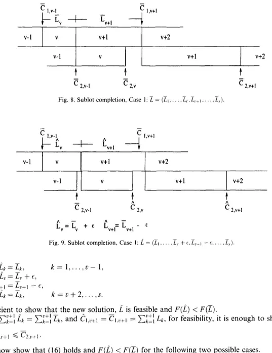
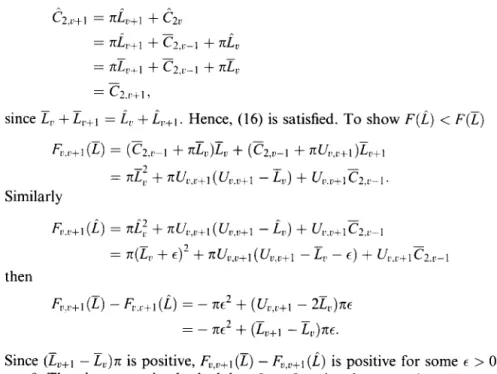
We will now show that (16) holds and F(L) < F(E) for the following two possible cases. Case 1: CI,~+~ > ??;2.r (see Figs. 8 and 9).

For small 6 > 0, we also have c,,V+l > &z;.~. ^

Cz.c’+l = &,+I + Cl.?+1 = n(L,.+, - E) + qc+, = &+, - rcnE.

(16)

Hence, Condition (16) is satisfied. To show F(i) < F(E), define F,,L3+l (L) to be the contribution of sublots I’ and v + 1 to the objective function and Uv.a+l = z,, + I,+, = i,. + &.+I.

58 A. @I et al. I European Journal of Operational Research 110 (1998) 4242

fi,v+l@) = [G,v-1 + E”( 1 + 7@,, + [(C,,“-1 + t,. + EL’+,) + 7tZ,+,]Lc+, = (1 + 71)Lf + (~u.o+, + 7&+1)L,+, + c,,v_l L$$!+,

= (1 + 42 + ~wJ+,L+1 + nL;+, + CIJ_l uc,o+, .

Similarly,

FL,,+, (i) = (1 + 7qi: + u”.o+,i”+l + nit+, + G.“Fl ~Lvfl

=

(1 + 7r)(E” + E)2 + Uv,v+,

(Lo+, - E) + @,,l - t)2 + Cl.“-, UlLv+l

then,

F,,,+,(E) - F,,,+,(i) = -(27c + 1)E2 + (27c + l)( U&“+, - 2L,)6

= -(27c + l)E2 + (27c+ l)(L,+, - L,)E.

But, we know that I& < TV+,, thus i?, < %+,, therefore it is clear that FL.,U+,

(I) - I$,+, (i) is positive for

some t > 0. Hence, F(E) > F(i), for some t > 0.

_-

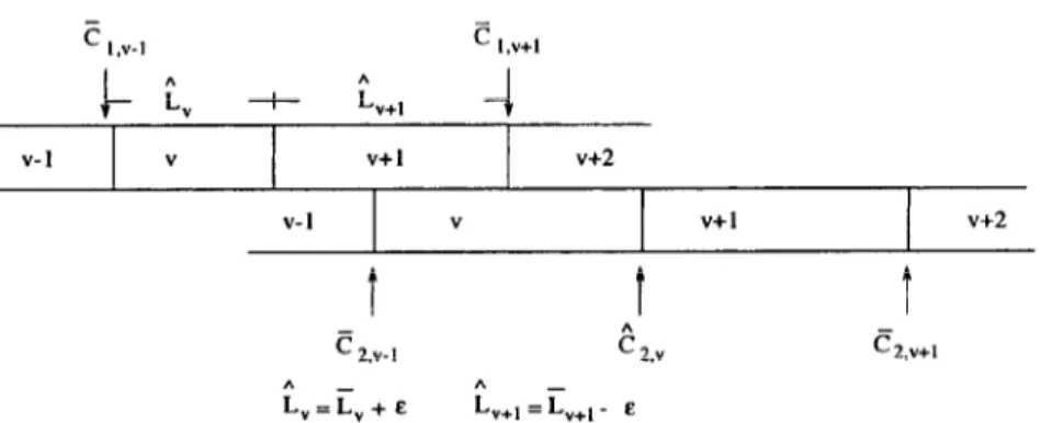
Case

2: Cl,“+, d c2,+ (see Figs. 10 and 11).

For E > 0 we also have Cl,“+, d

c2,0,

v-l

i” +

_L+*

-I

” v+l v+2 v-l V v+l v+2 t t T E _{2.vI C2.Y} c Z.v+l

Fig. 10. Sublot completion, Case 2: E = (11, ,L,,L,+I , ,Es).

s

I.%!-I

c

I,!!+1

J- i, + ;.

V+l

-4

V-l V v+l v+2 - -

c

2.wI

C2.”

c

Z.v+l

t,=i,+e

tV+, = iv+,

- E

A. $en et al. I European Journal of Operational Research 110 (1998) 42--62 59

since L,, + &.+I = i, +

i,,+t .

Hence, (16) is satisfied. To show F(L) < F(E) - -

Fr.,1+1 (Q = (G4 + xL,)L, + (G,“-1 + 7cU~,,+,)L,+, = nEf + 7cu,,,+l(ul..D+l -Z,) + Up.v+lCZ.a_,.

Similarly

F;W+l (L) = ZLf + ~~Lq!+t (UL’.v+l - 6,) + Ul..v+lCZ.a4

= n(L, + E)2 + nu,J+l(u~.cj+l - L,, - t) + U&u+,C2.r_,

then

&,,,>+I (L) - fi;.,C+l (i) = - 7ct2 + (L&+, - 2L,)rce = - 7cE2 + (L”,, - L&E.

Since (L,+t - LC)x is positive, F,,,+t (z) - &,+I (L) is positive for some E > 0. Thus, F(L) > F(L) for some t > 0. Thus in any optimal schedule, nLk 2 Lk+l k = 1,. . ,s - 1. 0

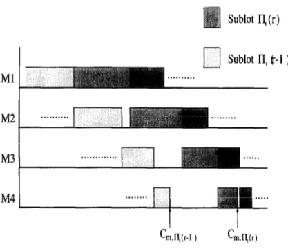
Having observed that rcLk 2 Lk+,, k = 1,. . , s - 1, for any optimal schedule, we can write the comple- tion time of each sublot on the second machine as (Fig. 12)

CZk=L, +rcCLp k= l,...,~. (=l

The mean flowtime is F(L) = 2 c2kLk k=l =-j-CL, +n&&k k=l Y=l =L1 k=l P=l 1 2 3 . . . k 1 2 3 . . . k-l k a t ‘2,k Fig. 12. Sublot completion, rrLk > Lk+, , k = 1, .S

60 A. Sen et al. I European Journal of Operational Research 110 (1998) 4262

Then, an equivalent reformulation of the problem is

min F(L) = LI + xC~,,C~&LP subject to clCILk = 1,

L k+l - ZLk < 0, k= l,...,s- 1,

Lk > 0, k= l,...,s.

Result 8.

The following sublot sizes are optimal for (17)-(20),

L1 =

3.-(s-u)

$y

n(s - v) +

($+,‘n ’

Lk =

&‘Z

,, k=l,..., o, l

=l-EIC;=,nr-l,

k=o+l .,, s k

b -

0)

>

7

(17)

(18)

(19) (20)

(21)

(22)

(23)

Proof.

The Gantt chart for an instance of the above sublot sizes will be as shown in Fig. 13. Since the ob- jective function can be shown to be convex, similarly as in the previous case, it will be sufficient to show that

the above solution is a Karush-Kuhn-Tucker point.

Assign, Lagrange multipliers 6 for (18) and & for (19). As seen in Fig. 13, only the first v - 1 of the type (19) constraints are binding. So Karush-Kuhn-Tucker conditions for the solution are:

For LI 1 + ?I + XL1 + 6 - 7G, = 0. ₍₂₄₎ FOl-Lk, k=2,...,v- 1 n+nLk+6+&, -n&=0. ₍₂₅₎ For L, 71+ 7cL, + 6 + A,_1 = 0. ₍₂₆₎ For&, k=v+l,...,s n + XLk + 6 = 0. ₍₂₇₎

We have the following solution to system (24)-(27). Using the values Z = (El, . . . , Es), and noting that &=& k=v+l,..., s,wegetfrOm(27),

V-2 V-l V vtl vt2 vt3 Vt4

v-3

V-2 V-l V vtl vt2 vt3

A. $en et al. I European Journal of Operational Resrarch I10 (1998) 42 62

6 = -7-c -

7&..

We also get from (26) and (28), I,._, = 7r(ZS - I,.). which is non-negative.

From (25) we obtain

ik = I&+, - 6 - lx- I&,, k= l....,u-2, ik = rc&+, + rc(tis - &+t), k = 1,. . , v - 2,

which together with (29), proves the non-negativity of ;lk, k = 1

/I, = (S)z- ($$)Z,.

On the other hand (24) and (28) give

( . . 0 - 2. We have from (29) and (30)

61 (28) (29) (30) (31) (32)

We also need to show that the sublot sizes result in a consistent solution of Lagrange multipliers

Using (23) z’-1 l-L,(3)

( >

n-1 _{( )} &-1 L =1_ (s - L’) - nz ’ 71 ) XII - 1

( 1

7c-l A-k= (S)l&+ ($+)I,,

which results in

z, =

$+r-(s-2))

$+

7T(s - u) +

(2)‘7c.

0

For u = s (i.e. all the sublot sizes are geometric), we have the system of equations (24)~(26). The system has a consistent solution, hence it is enough only to show the non-negativity of the Lagrange multipliers, &, k= l,..., s- 1. We have

62 A. ,Yen et al. I European Journal of Operational Research 110 (1998) 4242

is-, =

-+ + 27f+1 _+27c-2271-

₁

(rcs - 1)(7r + 1) c”e::, 7cy

’ s-k-l s-l ,tk = is_l c d+ c (L, - L,)&k. Y=O P=k+l

Since & > &t

k =

1,.

. . ,s -

2, it is sufficient to check the non-negativity of As-t.

Hence, all the sublot sizes are geometric (V = s), only if the polynomial in the numerator of 1,-t is po-

sitive for a given rr, since the denominator is always positive.

Combining these results, the following algorithm, repeated for convenience, solves the problem:

Algorithm 1 v c 0,

optimaltFALSE

If f(7c) = -7+ + 27?+’ + 27LS - 277 -

1 > 0

optimal c TRUE, geometric sublots are optimal

While not

optimal

v+-u+l

;, + [$=+I - (s - v)]/[$=+(s

- v) + ($+)‘7r]

k+n k-‘&, k=2,...,v

& + [l - z1 Xi=_! 7Cp1]/[(S - U)], k = U + 1,. . . ,S if 71 Z, > L,+l 3 L,,

optimal t TRUE, z = (Et,

. . . , Es)

is optimal

References

[I] K.R. Baker, Lot streaming to reduce cycle time in a flow shop, Working Paper 203, Amos Tuck School, Dartmouth College, 1988, Presented at the Third Annual Conference on Current Issues in Computer Science and Operations Research, Bilkent University, June 1988.

[2] D. Trietsch, Optimal transfer lots for batch manufacturing: A basic case and extensions, Technical Report NPS-54-87-010, Naval Postgraduate School, Monterey, CA, 1987.

[3] D. Trietsch, K.R. Baker, Basic Techniques for lot streaming, Operations Research 41 (1993) 106551076.

[4] C.A. Glass, J.N.D. Gupta, C.N. Potts, Lot streaming in three-stage production processes, European Journal of Operational Research 75 (1994) 378394.

[5] C.N. Potts, L. van Wassenhove, Integrating scheduling with batching and lot-sizing: A review of algorithms and complexity, Journal of Operational Research Society 48 (1992) 395406.

[6] C.N. Potts, K.R. Baker, Flow Shop scheduling with lot streaming, Operations Research Letters, 8 (1989) 297-303.

[7] F.C. Cetinkaya, J.N.D. Gupta, Flowshop lot streaming to minimize total weighted flow time, Research Memorandum 94-24, Industrial Engineering, Purdue University, 1994.

[8] D.H. Kropp, T.L. Smunt, Optimal and heuristic models for lot splitting in a flow shop, Decision Sciences 21 (1990) 691-709. [9] Engin Topaloglu, Alper Sen, ijmer Benli, Optimal streaming of a single job in a flow shop with two sublots, Research Report

IEOR-9412, Department of Industrial Engineering, Bilkent University, 1994.

[lo] M.L. Smith, S.S. Panwalkar, R.A. Dudek, Flowshop sequencing problem with ordered processing time matrices: A General case, Management Science, 21 (1975) 544-549.