A parallel progressive radiosity algorithm based on patch data circulation

(1)

Technical Section

A PARALLEL

PROGRESSIVE

RADIOSITY

ALGORITHM

BASED ON PATCH DATA CI:RCULATION

CEVDET AYKANAT,+ TOLGA K. CAPIN’ and BULENT 6ZGiiC Computer Engineering Department, Bilkent University, 0’5533 Bilkent, Ankara, Turkey

e-mail: aykanat@cs.bilkent.eclu.tr

Abstract---Current research on radiosity has concentrated on increasing the accuracy and the speed of the

solution. Although algorithmic and meshing techniques decrea,se the execution time, still excessive

computational power is required for complex scenes. Hence, parallelism can be exploited for speeding up the method further. This paper aims at providing a thorough examination of parallelism in the basic progressive refinement radiosity, and investigates its parallelization on distributed-memory parallel architectures. A synchronous scheme, based on static task assignment, is proposed to achieve better coherence for shooting patch selections. An efficient global circulation scheme is proposed for the parallel light distribution computations, which reduces the total volume of concurrent communication by an asymptotical factor. The proposed parallel algorithm is implemented on an Intel’s iPSC/2 hypercube

multicomputer. Load balance qualities of the proposed static assignment schemes are evaluated

experimentally. The effect of coherence in the parallel light distribution computations on the shooting patch selection sequence is also investigated. Theoretical and experimental evaluation is also presented to verify that the proposed parallelization scheme yields equally good performance on multicomputers implementing the simplest (e.g. ring) as well as the richest (e.g. hypercube) interconnection topologies. This paper also proposes and presents a parallel load re-balancing scheme which enhances our basic parallel

radiosity algorithm to be usable in the parallelization of radiosity methods adopting adaptive subdivision and meshing techniques. Copyright 0 1996 Elsevier Science Ltd

1. INTRODUCTION

Radiosity proposed by Goral et al. [I] is an

increasingly popular method for generating realistic

images of non-existing environments. The conven-

tional radiosity method is expensive in terms of

execution time and memory requirement, and the

final image cannot be viewed until the matrix

equation is solved. This reduces the usability of the

method for complex scenes consisting of a large

number of surfaces. The progressive refinement

radiosity proposed by Cohen et al. [2] allows viewing

of the approximated partial radiosity solutions

initially and approaches the correct solution iteratively. This new approach eliminates the construction of the linear system of equations, and follows the path the light travels in the environment. The initially approximated solutions are provided quickly and the final solution is approached iteratively. The following operations are performed at each iteration of the generic progressive refinement radiosity algorithm;

1. the most energetic surface is selected as the source surface,

2. form-factors from this source surface are computed,

+ Author for correspondence.

t Present address: Commuter Grauhics Lab (EPFL-LIG). Swiss Federal Institute o;Technoldgy, CH-lOiS Lausannd: Switzerland.

3. depending on these form-factors, light is distributed from source surface to environment.

Although. progressive refinement radiosity has

been successful at generating realistic-looking

images, it still has computation and modeling

requirements that limit the usage of the method for complex scenis. Several methods have been proposed in order to :speed up the solution by using preprocessing techniques for hierarchical representation of the

objects or by starting with coarse patches and

adaptively subdividing the necessary regions of the environment during the course of the solution. The initial work in adaptive subdivision is by Cohen et al. [3]. In this work, they propose a subdivision method called sub-structuring with hierarchical subdivision of the input surfaces into subsurfaces, patches and elements. Baum et al. [4] state the ultimate con-

straints required by the radiosity method and

propose an automatic subdivision method. Campbell and Fussell [5] present the subdivision for elimination

of light leakage. Hanrahan et al. [6] propose a

hierarchical representation of the environment. In their algorithm, the hierarchical radiosity is inspired by the N-Ilody problem, and the patch-to-patch visibility is computed and the form-factor computations are performed with required precision. Smits et al. [7] propose a view-dependent solution based on Hanrahan’s work. Lischinski et al. [8] propose an accurate radiosity based on discontinuity meshing. The mesh explicitly represents the discontinuities in

(2)

308 C. Aykanat, T. K. Capin and B. ozgiic the radiance function as boundaries between mesh

elements. Piecewise quadratic interpolation is used to approximate the radiance function. This solution is fully automatic and view-independent, and is not limited to constant-radiosity patches and produces a lesser number of patch elements.

Although algorithmic and meshing techniques decrease the execution time, still excessive computational power is required for complex scenes. Hence, parallelism can be exploited for speeding up the method further. This paper aims at providing a thorough examination of parallelism in the basic progressive refinement radiosity, and investigates its parallelization on distributed-memory parallel architectures (multicomputers). By basic radiosity algorithm we mean that the hierarchical and adaptive meshing techniques mentioned in the previous para- graph are not exploited during parallelization. The parallel algorithms proposed for the basic radiosity scheme depend on the static decomposition of the scene geometry generated during the preprocessing phase. However, we also propose and present a simple, yet effective parallel load re-balancing scheme to enhance our parallel algorithms to be usable in the parallelization of the radiosity methods adopting adaptive subdivision and meshing techniques. The main ideas proposed and presented in this paper can also be exploited in the parallelization of the hierarchical radiosity method. For example, the patch circulation and parallel light distribution schemes proposed in this paper can be exploited in the parallelization of the hierarchical radiosity method.

The hemicube algorithm proposed by Cohen and Greenberg [9] is used for form factor computations because of its simplicity, efficiency and possibility of its acceleration on current graphics hardware. The hemicube algorithm is an approximation method and the proximity, visibility and aliasing assumptions exploited in this algorithm may result in incorrect computation of the form-factors. In order to solve the problems caused by the hemicube method assumptions and compute more accurate form- factors, a number of form-factor computation techniques have been proposed. In Bu and Depret- tere’s approach [lo], the form-factor vector is computed by locating a hemisphere over the patch and casting rays towards the hemisphere pixels. Wallace et al. [ll] propose a source-to-vertex ray tracing solution. Instead of shooting rays from the source patch in the uniform directions of hemicube pixels, their method samples the shooting patch from the point of view of each other surface in the environment. From each vertex in the environment, rays are sampled towards different parts of the shooting patch, and tested for occlusions by other surfaces. Although the hemicube algorithm is used and discussed in this paper, the proposed parallelization approach is general enough to be valid for the parallelization of other form-factor computation schemes.

In a multicomputer, processors have only local memories and there is no shared memory. In these architectures, synchronization and coordination among processors are achieved through explicit message passing. Multicomputers have been popular due to their nice scalability feature. Various interconnection topologies have been proposed and implemented for connecting the processors of multicomputers. Among them, ring topology is the simplest topology which requires only two links per processor. Ring topology can easily be embedded onto almost all other interconnection topologies (e.g. hypercube, 2-D mesh, 3-D mesh, etc.). Hypercube topology has received considerable attention among other topologies. The popularity of the hypercube topology may be attributed to the following: (i) many other widely used topologies such as rings, meshes and trees can successfully be embedded onto a hypercube; (ii) in a d-dimensional hypercube with 2d= P processors, there exists d= log2 P connections per processor with a maximum distance of d between any two processors; and (iii) hypercube topology is completely symmetric and can be decomposed into sub-hypercubes allowing the efficient implementation of recursive divide-and-conquer algorithms. Hyper- cube can be considered as the richest interconnection topology adopted in the organization of commercially available multicomputers.

There are various parallel progressive refinement implementations proposed in the literature [12-181. Most of these approaches utilize asynchronous schemes based on demand-driven task assignment. The parallel progressive refinement algorithms proposed in this work utilize a synchronous scheme based on static task assignment [19]. The synchronous scheme is proposed in order to achieve better coherence during parallel light distribution computations. The proposed algorithms are implemented on an Intel’s iPSC/2 hypercube multicomputer. The organization of the paper is as follows. Section 2 summarizes the progressive refinement radiosity. Section 3 presents and discusses the proposed parallelization schemes for the basic progressive refinement radiosity algorithm. Section 4 presents a parallel load re-balancing scheme which enhances our basic parallel algorithms to be usable in the parallelization of the radiosity methods adopting adaptive subdivision and meshing techniques. Finally, experimental results are presented and discussed in Section 5.

2. PROGRESSIVE REFINEMENT RADIOSITY

Progressive refinement radiosity gives an initial approximation to the illumination of the environment and approaches the correct light distribution iteratively. Each iteration of the basic progressive refinement radiosity algorithm adopting the hemicube method for form-factor computations can be considered as a four-phase process:

(3)

2. production of hemicube item-buffers,

3. conversion of item-buffers to a form-factor vector, 4. light distribution using the form-factor vector.

In the first phase, the patch with maximum energy is selected for faster convergence. In the second phase, a hemicube [9] is placed onto this patch and all other patches are projected onto the item-buffers of the hemicube using the z-buffer algorithm for hidden patch removal. The patches are passed through a projection pipeline consisting of: visibility test, clipping, perspective projection and scan-conversion. In the third phase, the form-factor vector corresponding to the selected shooting patch is constructed from the hemicube item-buffers by scanning the hemicube and adding the delta form-factors of the pixels that belong to the same patch.

In the last phase, light energy of the shooting patch is distributed to the environment, by adding the light contributions from the shooting patch to the other patches. Distribution of light energy necessitates the use of the form-factor vector computed in Phase 3. The contribution from the shooting patch s to any other patch j is given by [2]:

j(r, g, b) = Bj(r, g, h) + Wr, g, b) (2)

ABAr, g b) = ABj(r, g, 6) + Wr, g, b) (3)

Here, AB,{r, g, 6) and r,{r, g, b) denote the delta radiosity and the reflectivity values, respectively, of patch j (for 3 color-bands), Aj denotes the area of patch i, and Fsj denotes the j ” element of the form- factor vector constructed in Phase 3 for the shooting patch s. During the execution of the algorithm, a patch may be selected as the shooting patch more than once. Therefore, the delta radiosity value (AB) is stored in addition to the radiosity (B) for each patch, which gives the difference between the current energy and the last estimate distributed from the patch. That is, it represents the amount of light the patch has gathered since the last shooting from the patch. The delta radiosity values are used for shooting patch selection. The iterative process is halted when the maximum or sum of ABiAi values of all patches reduce below a user-specified tolerance value.

3. PARALLELIZATION

As mentioned earlier, progressive refinement radiosity is an iterative algorithm. Hence, computations involved in an individual iteration should be investigated for parallelization while considering a proper interface between successive iterations. In this algorithm, strong computational and data dependencies exist between successive phases such that each phase requires the computational results of the previous phase in an iteration. Hence, parallelism at each phase should be investigated individually while

considering the dependencies between successive phases. Furthermore, strong computational and data dependencies also exist within each computational phase. T:lese intra-phase dependencies necessitate global interaction which may result in global interprocessor communication at each phase on a distributed-memory architecture. Considering the crucial gmnularity issue in parallel algorithm devel- opment for medium-to-coarse grain multicomputers, we have investigated a parallelization scheme which slightly modifies the original sequential algorithm. In the modified algorithm, instead of choosing a single patch, P shooting patches are selected at a time on a multicomputer with P processors. The modified algorithm is still an iterative algorithm where each iteration involves the following phases:

selection of P shooting patches, production of P hemicube item-buffers,

conversion of P hemicubes to P form-factor vectors,

distribution of light energy from P shooting patche:, using these P form-factor vectors. Note that the structure of the modified algorithm is very similar to that of the original algorithm. However, the computations involved in P successive iterations of the original algorithm are performed simultaneously in a single iteration of the modified algorithm. This modification increases the granularity of the computational phases since the amount of computation involved in each phase is duplicated P

times. Furthermore, it simplifies the parallelization since production of P hemicube buffers (Phase 2) and production of P form-factor vectors (F’hase 3) can be performed simultaneously and independently. Hence, processors can concurrently construct P form-factor vectors corresponding to P different shooting patches without any communication.

The modified algorithm is an approximation to the original progressive refinement method. The coherence of the shooting patch selection sequence is disturbed in the modified algorithm. The selection of

P shooting patches at a time ignores the effect of the mutual light distributions between these patches and the light d.istributions of these patches onto other patches during this selection. Thus, the sequence of shooting patches selected in the modified algorithm may deviate from the sequence to be selected in the original algorithm. This deviation may result in a greater number of shooting patch selections for convergence. Hence, the modification introduced for the sake of parallelization may degrade the performance of the original algorithm. This perfoxm- ante degradation is likely to increase with the increasing number of processors. This paper presents an experimental investigation of this issue.

This paper is based on this algorithmic modification of the sequential algorithm like some other parallel im:plementations proposed in the literature. However, these parallel implementations utilize

(4)

310 C. Aykanat, T. K. Capin and B. OzgiiG asynchronous schemes. These asynchronous schemes

have the advantage of minimizing the processors’ idle time since form-factor and light distribution computations proceed concurrently in an asynchronous manner. However, in these schemes, a processor, upon completing a form-factor vector computation for a shooting patch, selects a new shooting patch for a new form-factor computation. Hence, this asynchronous shooting patch selection by an individual processor does not consider the light contributions of the form-factor computations concurrently performed by other processors. Furthermore, large numbers of asynchronous communications with large volumes create congestion on the interconnection network, especially in simple topologies such as ring [ 131. In this work, we propose a synchronous scheme which is expected to achieve better coherence in the distributed shooting patch selections and eliminate message congestion. The proposed parallelization scheme is discussed in the following sections.

3.1. Phase I: shooting patch selection

There are two alternative schemes for performing this phase: local shooting patch selection and global shooting patch selection. In the local selection scheme, each processor selects the patch with maximum ABiAi value among its local patches. In the global selection scheme, each processor selects the first P patches with the greatest ABjAi values among its local patches in sorted order and interprocessor communication is performed in order to obtain the first P patches with maximum energy among these patches. Then, each processor selects a distinct shooting patch among these maximal patches. As will be discussed later, each processor is assumed to hold only a subset of the overall scene description. Thus, the local patches of an individual processor refers to N/P patches assigned to and stored by that processor assuming an even decomposition of a scene with N patches to P processors.

The number of shooting patch selections required for convergence of the parallel algorithm to the user- specified tolerance depends on the shooting patch selection scheme. Global scheme is expected to converge faster because the patches with globally maximum energy are selected. However, in the local scheme, the shooting patches that are selected may deviate largely, if maximum energy holding patches are gathered in some of the processors, while the other processors hold less energy holding patches. Hence, the global scheme is expected to achieve better coherence in distributed shooting patch selection. However, the global scheme requires circulation and comparison of P buffers, hence necessitating global communication overhead. Therefore, the global communication scheme should be designed efficiently considering the interconnection topology of the processors in order to minimize this overhead. In this work, we present efficient global patch selection schemes for the ring and hypercube topologies.

3.1.1. Ring topology. First, each processor selects the first P patches with the greatest ABiAi values among its local patches in sorted order and puts these patches (together with their geometry and color data) into a local buffer in decreasing order according to their ABiAi values. Then, these local buffers (each of size P) are circulated in P- 1 concurrent communication steps as follows. In each concurrent step, each processor merges its local sorted buffer of size P with the received sorted buffer of size P, discarding P patches with the lowest ABjAi values. Then, each processor sends its resulting buffer (of size P) to the next processor in the ring. Note that each processor keeps its original local sorted buffer intact during the circulation. At the end of P- 1 communication steps, each processor holds a copy of the same sequence of

P patches with globally maximum ABiA< values in decreasing order. Then, processor q selects the qfh

patch in its final patch list, for q = 0, 1, . , P- 1. Hence, processor q effectively selects the patch with the qfh largest ABiAi value as its shooting patch.

3.1.2. Hypercube topology. The parallel algorithm

for the hypercube topology is slightly different from the algorithm for the ring topology. The hypercube algorithm for global shooting patch selection uses the communication protocol generally used for global operations such as global sum, global maximum, etc. [20]. This scheme involves d=loglP concurrent exchange steps over channels i= 0, 1, , d- 1. Here, channel i refers to the set of P/2 communication links which connect processor pairs whose d-bit binary representations differ only in the ifh bit. In the 1 ‘I’ step, processors concurrently exchange their current sorted buffers (each of size P) with those of their neighbors over channel i. Then, processors concurrently merge the received sorted buffers with their current local sorted buffers discarding the P

patches with lowest ABiAi values. The resulting local buffers become the current sorted buffers for the following step of the algorithm. At the end of this procedure, each processor holds a copy of the same sequence of P patches with globally maximum ABiAi

values in decreasing order. Then, processor q selects the qth patch in its local sorted patch list, for q = 0, 1, “‘, P-l.

3.1.3. Performance analysis of Phase I. The parallel complexity of the communication phase for shooting patch selection on the ring topology is:

TyG ‘(P -- l)tsr, + (P - l)PTTR + (P - l)PTCOMP

(4)

where tsa is the message set-up time overhead, TTR is the transmission time for a single shooting patch data, T,o,, is the time to compare two patch entries of the arrays. Note that only P comparisons are enough to select the maximum P entries of two sorted arrays, each of size P.

(5)

311 On the hypercube topology, the algorithm given in

Section 3.1.2 decreases the total complexity by decreasing both the number and the volume of concurrent communications, and the number of comparison operations. The parallel complexity of the hypercube algorithm for this phase is,

TypER = dtsu + dPTTR + dPTCoMp. ₍₅₎

Thus, the hypercube topology performs better than the ring topology. However, computation time required by the shooting patch selection phase is negligible compared to the other phases discussed in the following sections. It will be shown that the other phases require O(N) time complexity, whereas the shooting patch selection phase requires O(p) complexity for the ring and O(P logzP) complexity for the hypercube topology. In general, N$P for complex scenes, and hidden constant factors in the asymptotic notations are substantially larger in other phases (especially in Phase 2). Hence, the performance increase introduced by the hypercube topology over the ring topology in this phase does not affect the performance of the overall parallel algorithm sig- nihcantly

3.2. Phase 2: hemicube production

In this phase, each processor needs to maintain a hemicube for constructing the form-factor vector corresponding to its local shooting patch. Further- more, each processor needs to access the entire scene description in order to fill its local hemicube item- buffers corresponding to its local shooting patch. One approach is to replicate the entire patch geometry data in each processor, hence avoiding interprocessor communication. However, this approach is not suitable for complex scenes with large numbers of patches because of the excessive local memory requirement of size O(N) per processor. Hence, a more valid approach is to evenly decompose the scene description into P patch data subsets and map each data subset to a distinct processor of the multicomputer, thus decreasing the local memory requirement per processor to O(N/P).

However, the decomposition of the scene data necessitates global interprocessor communication in this phase since each processor owns only a portion (of size N/P) of the patch database and needs to access the entire database. This requires circulating the patch subsets of the processors so that each patch data subset visits each of the P processors exactly once. Note that only geometry data of the patches are needed for projecting the patches in this phase and communication of the color information is unnecessary. Since messages can only be sent/received from/into con- tiguous memory locations in most of the commercially available multicomputers (e.g. iPSC/Z), the local patch data of each processor is divided into geometry and color parts. So, in Phase 2, only the local patch geometry data of the processors are circulated.

For a triangular meshing of the scene, geometry data of each triangular patch involves 3 floating- point words for each of its 3 vertices, 3 floating-point words for its normal, and one integer word for the patch-id. Hence, the geometry data for each patch requires .13 4-byte words (52 bytes in total) of storage. The color data of each patch involves one floating-point word for its area, 3 floating-point words for its (r, g, b) reflectivity values, and 6 floating-point words for its (r, g, b) radiosity and delta-radiosity values. Hence, the color data for each patch requires 10 4-byte words (40 bytes in total) of storage. Thus the proposed scheme, decreases the communication volume per triangular patch from 92 bytes to 52 bytes, thus achieving a ~43.5% decrease in the total volume of communication in Phase 2. The following subsections present the patch circulation algorithm:: for ring-connected and hypercube-con- netted multicomputers.

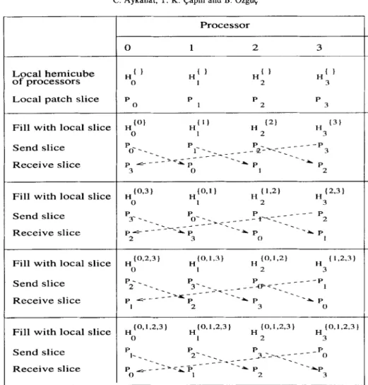
3.2.1. Ring topology. Patch circulation needed in this phase can be achieved in P concurrent communication sieps as follows. In each step, processors concurrently project their current patch data subsets onto their local hemicubes. Then, they concurrently send these patch data subsets to their next processors on the ring. Patch data subsets received from the previous processors on the ring become the current patch data subsets for the next step. At the end of P

concurrent communication steps, each processor completes the projection of all patches onto its local hemicube. Although P- 1 communications would be enough for this operation, one more communication is required in order to return all geometry data subsets to their home processors for maintaining the storage consistency of geometry and color data subsets for subsequent iterations and rendering.

Figure 1 illustrates the execution of the algorithm on a ring with 4 processors. In this figure, P4 denotes the qfh subset of the patch geometry data which corresponds to the original local patch data subset of processor (I, and Hi denotes that the local hemicube of processor q has been filled by the local patch data subsets of the set J of processors.

We present two interprocessor communication schemes for the implementation of the synchronous patch data circulation in this phase: tightly-coupled and loosely-coupled. In the tightly-coupled scheme, each processor delays sending its current patch data subset until it completes the projection computations associated with those patches. This scheme introduces processor idle time if the projection computations associated with the current patch subset of the destination processor are less than those of the sending processor. The loosely- coupled scheme is introduced to reduce the processor idle time. In this scheme, processors divide their current patch data subsets into two halves. Each processor sends the appropriate half as soon as it completes the projection operations associated with that half. Then, it proceeds to process the: other half after issuing a non-blocking

(6)

312 C. Aykanat, T. K. Capm and B. Ozgiiq

Local hemicube of processors

Local patch slice

Fill with local slice Send slice

Receive slice

Fill with local slice Send slice Receive slice Processor 0 1 2 3 P P P P 0 1 2 3 H (01 H(Il H (21 H (3) 0 1 2 3 P 0---__ P 1--- p L-- -I:,,--- -z--e--- _ -p2-_y~- - - - -P 3 -. P --A P -i p 3 0 1 2 “(0.3) H{o.ll H 11.2) H (2.31 0 1 2 3 P P P _---- p 3- - _ _{-_} o--,~~~~---t--~;~ 2 .---- - - -._ -. p&--- _+P _-A _p --A p 2 3 0 1 H 10.2.3) “(0,1,3) H to.1.21 H (1.2.3) 0 I 2 3 P2-- _-. P P ---p --_ 3~--~=_- _ - --a-=;-- 1 p 4--- ---a--- P -__ AP -. --A p I 2 3 0 Hto,1.2,3) “(0,1,2,3) H to.1 v2.3) H {0,1,2,3) 0 I 2 3 P P P I-__ 2‘ _ _ -P 0 -. -:a<--- --.J>-:-- _ ,3----,= - - - - -. P L- - *P -* p --Ap 0 1 2 3

Fig. 1. Patch circulation on a ring with 4 processors

receive into the memory area corresponding to the former half (that is already processed and sent).

Thus, messages arriving to the destination pro-

cessors usually find pending non-blocking receives, hence enabling the overlapping of receive operations with local computations on a cycle-stealing

basis. However, blocking send mode should be

used in order to prevent the arriving message to

contaminate the message being sent. Note that

both schemes use in-place communications since

they do not necessitate any extra send/receive

buffer.

Xd = Xd-l(d - I)&-, , ford> 1, whereXr =0

(6)

3.2.2. Hypercube ropology. For MIMD hyper-

cubes, patch circulation can be achieved by embedding the ring onto the hypercube using Gray Code ordering scheme. However, this embedding utilizes different channels of the hypercube for the communication between successive processors of the em-

bedded ring. This necessitates d successive

communication steps to achieve a single concurrent shift in the ring embedded on SIMD hypercubes. An efficient circulation scheme for a d-dimensional

SIMD hypercube can be achieved with the use of

exchange sequence X, [21]:

For example, X2= (0, 1, 0) and XJ = {0, 1, 0, 2, 0, 1, 0) are the exchange sequences for 2-D and 3-D

SIMD hypercubes, respectively. The exchange

sequence X, specifies the sequence of bidirectional

channels to be used for interprocessor commu-

nications in successive concurrent exchange

communication steps. The recursive definition of

the exchange sequence X, states that the d-

dimensional hypercube is divided into two d- 1

sub-hypercubes over channel d- 1 (represented by

the X,-r subsequences). In the first phase corresponding to the prefix subsequence Xd- r, patch

data circulation is performed independently and

concurrently in these two d- 1 dimensional sub-

cubes using the exchange sequence X,- ,. Then, in

the second phase, processors of these two sub-

cubes exchange their current patch data subsets

with each other over channel d- 1. In the last

phase corresponding to the postfix subsequence

(7)

Processor

0 1 2 3 4 5 6 7

Local hemicube H H H H H H H H

of processors 0 2 3 4 5 6 7 x3

Local patch slice P P P P P P P P

0 2 3 4 5 Ii 7

Project & send slice P u:=:” -P I

“A

Receive new slice ‘T’ ‘o

P . _,P P. _.P P . P 2 ..,,I 3 4‘. ,’ 5 h *. I’ 7 ,a PA’ ,’ .‘A I-\ PA’ .A , P P P L’ .~ P 0 3 2 5 4 1 6

Project s( send slice P.;. ‘.,’ ,‘pq P . I \. ,’ ,P II P \ 7 ‘.*,’ ,P 6 P \ 5 -. I’ ,P 4 ,’ -. ,I. PK aP pK’ ‘Ap .’ -\ pkx’ *p ,,l-.A 0

Receive new slice P

4’ P

2 3 (I I 6 7 4 5

Project Rr send slice P 6‘. -*‘7 P 4‘.. ,’ .P 5 P. 2‘. ,’ ,P 3

,‘-‘. .%. ;z

Receive new slice ‘7’

0

2

Project Kr send slice P _ 7 --. 4 P _ 3 --_ _.z<2-- -.;=--P ;_>.y- P -P (1 -. -

LT-- &-- ;/-- -. _I

Receive new slice ’ P P %P -P

5 4 7 6 0 3 2

Project Kr send slice P. 5‘. ,’ ,P 4 P. 7 -. *’ ,P h P. I’.\ ,T’ P 0 P.;. ,,-p 2

=: :>r

, Receive new slice

‘2’ ‘A ,*4‘.4

P 5 P L’ 6 P 7 Pfi 0 ,‘^\A P P fl 2 .4 P 3 0

Fig. 2. Patch circulation on a 3-D hypercube.

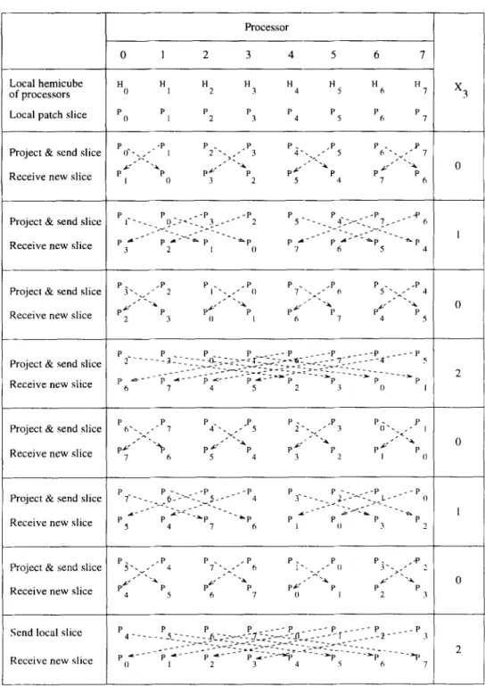
pendently and concurrently in these two d- 1 3.2.3. Performance analysis of Phase 2. The parallel

dimensional subcubes using the exchange sequence algorithms given for the ring and the hypercube

Xd- i. Note that P- 1 communication steps are topologies both require P concurrent communica-

enough for circulating all the patches so that each tions and a communication volume of N/P patch

patch subset visits all the processors. One more geometry data in each concurrent communication.

exchange communication over channel d- 1 is Hence, the efficiency of this phase is independent of

required to return all patch data subsets to their the interconnection topology of the processors, so the

home processors for maintaining patch data storage performance of this phase does not degrade with

consistency. Figure 2 illustrates this patch circula- simple topologies. It follows that the parallel com- tion scheme on a 3-D hypercube with 8 processors. plexity of Phase 2 is:

(8)

314 C. Aykanat, T. K. Capm and B. Ozgiic

Tp2 = Pku + W/f') T$-,q + W/P) TPROJ = Ptsu t NT& t NTPROJ (7)

Here, T”TR is the time taken for the transmission of the geometry data of a single patch, T~ROJ is the average time taken to project and scan-convert one patch onto a hemicube.

There are two crucial factors that affect the efficiency of the parallelization in this phase: load imbalance and communication overhead. Note that the parallel complexity given in Eq. (7) assumes a perfect load balance among processors. Mapping equal number of patches to each processor achieves balanced communication volume at each concurrent communication step. Furthermore, as will be discussed later, it achieves perfect load balance among processors in the parallel light distribution phase (Phase 4). However, this mapping may not achieve computational balance in the parallel hemicube production phase (Phase 2).

The complexity of the projection of an individual patch onto a hemicube depends on several geometric factors. Recall that each patch passes through a projection pipeline consisting of visibility test, clipping, perspective projection and scan-conversion. A patch which is not visible by the shooting patch requires much less computation compared to a visible patch since it leaves the projection pipeline in a very early stage. The complexity of the scan-conversion stage for a particular patch depends strongly on the distance and the orientation of that patch with respect to the shooting patch. That is, a patch with larger projection area on a hemicube requires more scan-conversion computations than a patch with a smaller projection area. As mentioned earlier, each iteration of the proposed algorithm consists of P

concurrent steps. At each step, different processors concurrently perform the projection of different patch subsets onto different hemicubes. Hence, the decomposition scheme should be carefully selected in

order to maintain the computational load balance in this phase of the algorithm.

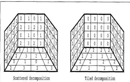
Two possible decomposition schemes are tiled and scattered decompositions. In the tiled decomposition, the neighboring patches are assigned to the same processors. This type of decomposition can be achieved in the following way: assuming that the patches that belong to the same surface are supplied consecutively, the first N/P patches are allocated to processor 0, the next N/P patches are allocated to processor 1, and etc. At the end of the decomposition, each processor stores almost equal number of patches in its local memory. In the scattered decomposition, the neighboring patches are stored in different processors, therefore the patches that belong to a surface are shared by different processors. Scattered decomposition can be achieved in the following way: again assuming that the neighbor patches belonging to the same surface are supplied consecutively, the incoming patches are allocated to the processors in a round-robin fashion. That is, the first patch is allocated to processor 0, the next to processor 1, etc.

When P patches are allocated, the next incoming patch is allocated to processor 0, and this process continues. When the decomposition is completed, first N mod P processors store [N/P] patches, while the remaining processors store LN/P] patches in their local memories. Figure 3 illustrates the scattered and tiled decompositions of a simple scene consisting of four faces of a room. The numbers shown inside the patches indicate their processor assignments for a 4 processor multicomputer.

Assuming that neighbor patches require an almost equal amount of computation for projection on different hemicubes, the scattered decomposition is expected to produce patch partitions requiring an almost equal amount of computations in Phase 2. So, it can be expected that the scattered decomposition

achieves a much better load balance than the tiled decomposition in Phase 2.

Scattered

decomposition

Tiled decomposition

Fig. 3. Scattered and tiled decomposition schemes

(9)

315 Communication overhead in this phase consists of

two components: number of communications and volume of communications. Each concurrent communication step adds a fixed message set-up time overhead tSu to the parallel algorithm. In medium grain multicomputers (e.g. Intel’s iPSC/2 hypercube) tSU is substantially greater than the transmission time tTR where tTR denotes the time taken for the transmission of a single word. For example, tsuz 550 p, where ~TR z 1.44 ps per 4-byte word in iPSC/2. Note that T gTR = 13tTR in Eq. (7), since the communication of an individual patch geometry involves the transmission 13 4-byte words.

However, as seen in Eq. (7), the total number of concurrent communications at each iteration is equal to the number of processors P, whereas the total volume of concurrent communication is equal to the number of patches N. Hence, the set-up time overhead is negligible for complex scenes (NFP). Then, assuming a perfect load balance, efficiency of Phase 2 can be expressed as:

&=1

PNTPROJ p PNTPRoJ+P~sL,+ NT”rR NTPROJ NN NTPRoJ+NT& TPROJ 1 =- = TPROJ+ T$R 1 -+%~TPRoJ

since one iteration of the parallel algorithm is computationally equivalent to P iterations of the sequential algorithm. Equation 8 means that projection of an individual patch onto a hemicube involves the communication of its geometry data as an overhead. As seen in Eq. (8), the overall efficiency of this phase only depends on the ratio TtR/TpRoJ

for sufficiently large N/P. For example, efficiency is expected to increase with increasing patch areas and increasing hemicube resolution, since the granularity of a projection computation increases with these factors.

In this work, we have also developed and implemented a demand-driven (asynchronous) patch circulation scheme for the experimental performance evaluation of the proposed loosely-coupled synchronous scheme with scattered decomposition. The proposed demand-driven implementation exploits both the rich hypercube topology and the direct- routing feature of iPSC/2 architecture. The direct- routing hardware of iPSC/2 almost achieves single- hop communication performance on multi-hop communications by avoiding the interception of intermediate processors. In this scheme, as soon as a processor completes the projection of its current patch subset it makes a request to another processor (in a deterministic order). When a processor receives a request, it sends its initially assigned local patch subset to the requesting processor. Processors reply requests in interrupt-driven mode in order to mini-

mize the idle time of the requesting processor. Non- blocking sends are used during these replies in order to overlap send operations with the local computations. Ths scheme necessitates an extra local memory space of size @N/P) in each processor to hold the current patch subset to be received upon request in addition to the initially assigned patch subset. Note that extra memory space will be needed in the processors of a hypercube multicomputer which utilizes store-and-forward type software routing for handling multi-hop messages since intermediate processors are intercepted in such routing schemes. Hence, this scheme is not efficient for multicomputer architectures which do not implement the direct routing scheme. This demand-driven scheme is also not efficient for parallel architectures implementing simple interconnection topologies (e.g. ring) due to network congestion.

3.3. Phase 3: form-factor vector computation

In this phase, each processor can concurrently compute the form-factor vector corresponding to its shooting patch using its local hemicube item-buffers constructed in the previous phase. This phase requires no interprocessor communication. Local form-fact’or vector computations involved in this phase require scanning all hemicube item-buffer entries. Hence, perfect load balance is easily achieved since each processor maintains a hemicube of equal resolution.

3.4. Phase 4: light distribution

At the end of Phase 3, each processor holds a local form-factor vector corresponding to its shooting patch. In this phase, each processor should compute the light contributions from all P shooting patches to its local Ipatches. Hence, each processor needs all form-factor vectors. Thus, this phase necessitates global interprocessor communication.

We introduce a vector notation for the sake of clarity of the presentation of the algorithms discussed in this section. Let X, denote the qth slice of a global vector X assigned to processor q. For example, each processor q can be considered as storing the qth slice of the global array of records representing the entire patch geometry data. In this notation, each processor q is responsible for computing the qrh slice AB, of the global contribution vector AB in order to update the qfh slices B, and AB, of the global radiosity and delta radiosity vectors B and AB, respectively. The notation used to label the i3 distinct form-factor vectors computed by

P processors is slightly different. In this case, Fp denotes the form-factor vector computed by processor p and F; denotes the qth slice of the local form-factor of processor p. In other words, F: denotes th.e form-factors from the shooting patch of processor p to the local patches of processor q.

As seen in Eq. (I), red, green and blue reflectivity values and the area of each patch i are needed as three ratios r,ir, g, b)/Ai in the contribution computa-

(10)

316 C. Aykanat, T. K. Capin and B. bgiiq tions. Hence, each processor q computes these three

ratios for each local patch and stores them into a local vector rq(r, g, b) (of size N/P) during preprocessing. That is, each processor q can be considered as holding the qth slice r&r, g, b) of the global vector r(r, g, b) which contains these constants for all patches. Hence, in vector notation, each processor q, for q = 0, 1, , P- 1, is responsible for computing P-l &(r, g, b) = c W(r, g, b)A:(q(r, g, b) x F$) p=o (9) %(r, g, b) = B,(r, g, b) +bR,(r, g, b) (10)

&(r, g, b) = AB,(r, g, b) +&(r, g, b) (11) where Aq(r, g, b) and A! denote the delta radiosity values for three color-bands and the area of the shooting patch of processor p. In Eq. (9) “x” denotes the element-by-element multiplication of two column vectors. As seen in Eqs (10) and (1 l), radiosity and delta-radiosity update computations are local vector additions which do not require any interprocessor communication. It is the contribution computation phase (Eq. 9), which requires global interaction. Equation (9) can be rewritten by factor- ing out the r4 vector as

UP,(r, g, b) = Aq(r, g, b)4’F:

forp=O, 1, . . . . P- 1 (12) P-l U,(r, g, b) = C Up,(r, g, b) (13) pal %(r, g, b) = dr, g, b) x U,(r, g, b) (14) Note that the notation used to label the U vectors is similar to that of the F vectors. That is, U:(r, g, b) (of size N/P) represents the contribution vector of the shooting patch of processor p to the local patches of processor q omitting the multiplications with the respective local r,{r, g, b)/Aj coefficients. Hence, U,(r, g, b) (of size N/P) represents the total contribution vector of all P shooting patches to the local patches of processor q, omitting the multiplications with the respective local r,{r, g, b)/Aj coefficients. The following sections present the ring and hypercube algorithms for performing this phase.

3.4.1. Ring topology. The first approach discussed in this work is very similar to the implementation proposed by Chalmers et al. [13]. In their implementation, each processor p broadcasts a packet consisting of the delta radiosities, area and the form-factor vector of its shooting patch. Each processor q, upon receiving a packet {Aq, A:, Fp}, computes a local contribution vector U$(r, g, b) by performing a local

scalar vector product for each color (Eq. 12) and accumulates this vector to its local U&r, g, b) vector by performing a local vector addition operation (Eq. 13). However, multiple broadcast operations with high volumes are expensive and may cause excessive congestion even in rich interconnection topologies. In this work, indicated packets are circulated in a synchronous manner, similar to the patch circulation scheme discussed for Phase 2. This circulation operation requires P- 1 concurrent communication steps. Between each successive communication step, each processor concurrently performs the contribution vector accumulation computations (Eqs 12 and 13) corresponding to its current packet. At the end of

P- 1 concurrent communication steps, each processor q accumulates its total contribution vector U,(r, g, b). Then, each processor q can concurrently compute its local AR,(r, g, b) vector by performing a local element-by-element vector multiplication for each color (Eq. 14).

It is obvious that perfect load balance in this phase can easily be achieved by mapping an equal number of patches to each processor. Hence, the parallel complexity of Phase 4 using the form-factor vector circulation scheme is,

Tp4 = (P- l)tsu + (P - l)Ntl, + P(N/P)TCoNrR

+ (NIP) TLIPD

= (p - lhu + (p - l)Ntl, + NTcaNrR

+ (N/f’) TC/PD

Here, tt, is the time taken to transmit a single floating point word, TCON~R is the time taken to compute and accumulate a single contribution value, and TUpD is the time taken to update a single radiosity and delta radiosity value using the corresponding entry of a local U, vector.

Note that, in this scheme, processors accumulate the contributions for their local patches during the circulation of form-factor vectors. Hence, as also seen in Eq. (15), this scheme necessitates high volume of communication ((P- l)N words) since entire form- factor vectors, each of size N, are concurrently communicated at each communication step. However, as also seen in Eqs (12) and (13), each processor q

needs only the qfh slices (each of size N/P) of the form- factor vectors it receives during the circulation. That is, the form-factor circulation scheme involves the circulation of redundant information. In this work, we propose an efficient scheme which avoids this redun- dancy in the interprocessor communication. In the proposed scheme, partial contribution computation results, Uz(r, g, b) vectors (each of size N/P), are circulated instead of the form-factor vectors (each of size N). Hence, each processor effectively accumulates the contributions of its local shooting patch to all other processors’ local patches during the circulation of the partial contribution computation results.

(11)

In a straightforward implementation of the proposed scheme, each processor q first constructs the contribution vector Ui(r, g, b) of its shooting patch to its local patches, and initiates the circulation of contribution vectors. After the ith concurrent com-

munication step in the circulation, processor q

;;;:y the uyq-l”odP (r, g, b) vector using the

(q-i)modP of its ocal form-factor vector Fq, and

accumulates this vector to the current partial

contribution vector. At the end of P- 1 concurrent communication steps, each processor q holds the final contribution vector U~q+t)mo&r, g, b) of the next processor in the ring. Hence, one more communication is needed in order to return the final contribution vectors to their home processors. However, this final

communication step can be avoided by each pro-

cessor q constructing U~q~~dOJr. g, b) vector in ;k;

initialization phase accumulating

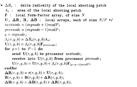
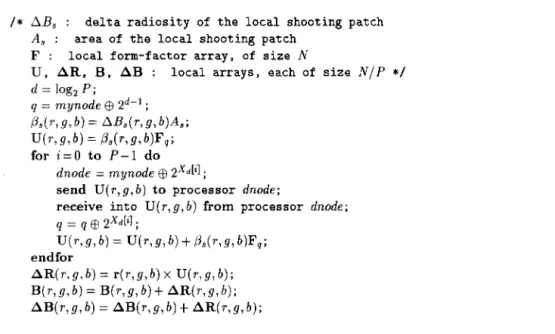
yq-i- 1 )modP(r’ g, b) vector at step i. Figure 4 illustrates the node program (in pseudocode) of the proposed contribution vector circulation scheme for the ring topology. In this pseudocode, the local variable mynode is assumed to contain the index of the respective node processor. Note that U, AR, B, and AB represent local arrays, each of size N/P, in the pseudocode in contrary to the global vector notation used in the texl..

3.4.2. Hypercube topology. The algorithm pro-

posed for the SIMD hypercubes is similar to that for the ring topology. This phase again requires the exchange sequence introduced for Phase 2 in order to

circulate the partial contribution computation

results. Figure 5 illustrates the node program (in

pseudocode) of the proposed contribution vector

circulation scheme for the hypercube topology. In

Fig. 5, Xdij denotes the ifh channel in the exchange sequence & defined in Eq. (6).

3.4.3. Performance analysis of Phase 4. As seen in Figs 4 and 5, the contribution vector circulation schemes proposed for ring and hypercube topologies

both require P- 1 concurrent communications and a

communication volume of 3N/P floating point words

at each concurrent communication. Both schemes

preserve the perfect load balance, if exactly equal number of patches are mapped to each processor. Hence, tke efficiency of this phase is also independent of the interconnection topology of the processors. Thus, the performance of this phase does not degrade with simple topologies. It follows that the parallel complexi;:y of Phase 4 is:

Tp4 =: (p - l)tsu + 3(P - 1) (N/P)t,,

l

P(NIP)TCONTR + (N/ P)T”~D

=: (P- l)tsr,+3 y _{Nto t NTCONTR}

N

fp TUPD

Note thal: the constant 3 appears as a coefficient in the “t(,” term since each entry of an individual U: vector consists of 3 contribution values for 3 color-

bands. Comparison of Eq. (16) with Eq. (15)

confirms that the proposed contribution vector

circulation scheme reduces the total concurrent

communication volume in Phase 4 by an asympto-

tical factor of P/3, for P>3, compared to the form- factor vector circulation scheme.

As seen in the for-loops of Figs 4 and 5,

/* AB, : delta radiosity of the local shooting patch ‘4, : area of the local shooting patch

F : local form-factor array, of size N

U, AR, B, AB : local arrays, each of size NIP */

nextn,ode = (mynode •t 1)modP; p-evn.ode = (mynode - 1)nrodP; y = mynode;

iMr,g,b) = ABs(T,g,bMs; U(T, g, b) = b’s(r, g, ~)Fpreunode; for p:= 1 to P-l do

send U(r,g,b) to processor neztnode;

receive into U(r,g,b) from processor prevnodc; U(T,g,b)= U(T,g,b)+p,(T,g,b)F(q--p--l)modP;

endfor

AR(r,g,b) = r(r,g,b) x U(r,g,b); Wr,g,b) = B(r,g,b)t AR(r,g,b); .4B(~.g,b) = AB(T,g,b)+ AR(r,g,b);

(12)

318 C. Aykanat, T. K. Capm and B. Ozgiig

/* AB, : delta radiosity of the local shooting patch

A, : area of the local shooting patch

F : local form-factor array, of size N

U, AR, B, AB : local arrays, each of size N/P */ d = log,P;

q = mynode $ 2d-1 ; Ps(r,g,b) = AB.dT,g,b)As; U(r,g,b) = Ps(T,g,bP’,;

for i=O to P-l do

dnode = mynode $ 2Xd[i] ;

send U(r,g, b) to processor dnode;

receive into U(r,g, b) from processor dnode;

9 = * @ ‘p&l ;

U(r,g,b) = U(r,g,b)+ Bs(r,g,b)F,;

endfor

ANT, 9, b) = r(T,g, b) x U(r, g, b); B(r,g,b) = B(r,g,b)+ AR(r,g,b); AB(~,g,bj = AB(r,g,b) t AR(r,g,b);

Fig. 5. The contribution vector circulation scheme for the hypercube topology.

computation and accumulation of a single contribution val;e (except the initialization) require 1 multiplication and 1 addition operation, for each color-band, at each step. Hence, TCoNTR = (3 x 2)t,,/,

= 6tcnro where tcalc denotes the time taken by

floating-point multiplication and addition operations. As also seen in these two figures (after the

for-loops), updating a single radiosity and delta-

radiosity value using the respective entry of the local U array requires 1 multiplication and 2 addition operations for each color-band. Hence,

Similar to the efficiency analysis of Phase 2, the set- up time overhead becomes negligible for sufficiently large granularity values (N/P&-). Then, the efficiency of Phase 4 can be expressed as:

1

Ep4 =- PWCONTR + TUPD)

P NTCONTR +(N/P)TuPD+P~s~+~N~,, TcONTR+ TUPD 52 TCONTR + TuPD/~+ 3trr 1 %dc = 6tcarc + %czdP + % 1 = 0.4 + 0.6/P + 0.2(trr/tcalc) (17)

since one iteration of the parallel algorithm is computationally equivalent to P iterations of the sequential algorithm. Note that rj(r, g, b)/Aj values, for all patches, are also assumed to be computed and stored during the preprocessing phase of the sequen-

tial algorithm. As seen in Eq. (17), the efficiency of the proposed contribution vector circulation scheme increases with increasing number of processors for a fixed granularity (N/P). Furthermore, this scheme will yield superlinear speedup (efficiency value greater than 1) for a wide range of machine specific ttr/tcalc values. For example, even for P=2, superlinear speedup can be obtained for t,,/tcalc< 1.5 (e.g. t,r/tCo~cz 1.44 pet/5.8 psecw0.25 in iPSC/2). The

superlinear speedup in this phase may appear to be

controversial since the conventional algorithm performs P radiosity and delta-radio&y update computation phases, whereas the modified algorithm performs only one update computation phase, for P

shooting patch selections. However, this analysis is still valid since it is not rational to use the modified algorithm on sequential computers and the performance degradation of the parallel algorithm due to this modification is also included in its experimental performance evaluation.

4. LOAD REBALANCING FOR ADAPTIVE SUBDIVISION

In this section, we propose a simple, yet effective

parallel load re-balancing scheme to enhance our parallel algorithms to be usable in the parallelization of the radiosity methods adopting adaptive subdivision and meshing techniques.

Assume that at the beginning of a particular iteration k first Qk = Nk mod P processors, 0, 1, . . . , Qk- 1, store [Nk/P’J patches, while the remaining processors, Qk, Qk+], . . , P- 1, store INk/P]

patches in their local memories. Here, Nk denotes the total number of patches to be processed in the current iteration k including the subpatches obtained

(13)

(14)

320 C. Aykanat, T. K. Capm and B. Ozgiiq

beginning of the next iteration k+ 1. Here, Nk+, = Nk + Mk denotes the total number of patches to be processed at iteration k+ 1. Hence, the proposed scheme restores the even distribution of the patches while maintaining the nice scattered decomposition at the beginning of each iteration. Note that each processor should know Qk+ 1 for the load re-balancing operation to be performed at the end of iteration k + 1. It is sufficient to have processor P- 1 compute and broadcast Qk+ I= (Qk + Mk) mod

P since it already has spW1 =Mk. This broadcast operation requires P- 1 left or right shift operations on the successive processors of the ring starting from processor P- 1.

Communication overhead introduced during the circulation of patch radiosity values is negligible since only two words (one integer and one floating-point word) are circulated for each patch. Communication overhead introduced during the subpatch circulation operation can also be considered as negligible if

Mk < Nk during the iterations. Hence, calculations and communication operations (circulation, prefix- sum and broadcast) performed for computing the vertex radiosities and re-assignments for the generated subpatches introduce negligible overhead to the overall parallel algorithm. Thus, the advantage of hypercube topology over ring topology does not matter although both prefix-sum and broadcast operations can be performed in d= log, P concurrent communication steps in hypercubes [21]. However, all-to-all personalized communication schemes proposed in the literature [22] can be exploited to reduce the communication volume overhead in the re- assignment phase on MIMD type hypercubes implementing direct routing (circuit-switching).

5. EXPERIMENTAL RESULTS

The proposed parallel algorithms are implemented and tested on rings embedded on an Intel’s iPSC/2 hypercube multicomputer. Only the demand-driven scheme discussed for Phase 2 is implemented and tested on the hypercube topology using the direct- routing feature of iPSC/2.

The form-factors are computed using hemicubes of constant resolution 50 x 100 x 100. The proposed

parallel algorithms are experimented for six different scenes with 522, 856, 1412, 3424, 5648 and 8352 patches. The test scenes are selected as house interiors consisting of objects such as chairs, tables, etc. in order to represent a realistic 3-D environment.

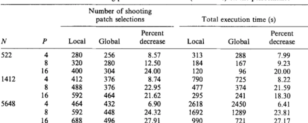
Table 1 illustrates the effect of the local and global shooting patch selection (in Phase 1) on the convergence of the parallel algorithm. As seen in Table 1, global selection scheme decreases both the

total number of shooting patch selections and the parallel execution time significantly. As seen in this table, percent decrease in the parallel execution time is slightly smaller than the percent decrease in the total number shooting patch selections for each instance due to the small computational and communication overhead of the global scheme compared

to the local scheme.

Table 2 shows the effect of the decomposition scheme on the performance of the hemicube production phase (Phase 2) of the parallel algorithm. Efficiency values in Table 2 are computed using:

Ej”ciency = TsEQ/(PT~AR) ₍₁₈₎

Parallel timing ( TPAR) in Eq. (18) denotes the average parallel hemicube production time per shooting patch. These timings are computed as the execution time of P concurrent hemicube productions divided by P since P hemicubes are concurrently produced for P shooting patches in a single iteration of Phase 2. Sequential timing (TsEQ) in Eq. (18) denotes the average sequential execution time of a single hemicube production. Hence, in Table 2, an efficiency value denotes the quality of a decomposition scheme on the load balance. .4s seen in Table 2, scattered decomposition always achieves better load balance than the tiled decomposition. Note that as the number of processors increases, load balance quality of the scattered decomposition increases in comparison with that of the tiled decomposition. Further- more, the performance of the loosely-coupled approach is almost always better than the tightly-

Table 1. Effect of the shooting patch selection scheme (in Phase 1) on the performance Number of shooting

patch selections Total execution time (s)

Percent Percent

N P Local Global decrease Local Global decrease

522 4 280 256 8.57 313 288 7.99 8 320 280 12.50 184 167 9.23 16 400 304 24.00 120 96 20.00 1412 4 412 316 8.74 790 725 8.22 8 488 316 22.95 417 374 21.59 16 592 464 21.62 295 241 18.30 5648 4 464 432 6.90 2618 2450 6.41 8 592 448 24.32 1692 1289 23.81 16 688 496 27.91 990 721 27.17

(15)

Table 2. Effect of the decomposition scheme on the performance (in terms of efficiency) of the hemicube production phase (Phase 2)

Synchronous (ring)

Tiled Scattered Asynchronous

demand

Tightly Tightly Loosely driven

N P coupled coupled coupled (hypercube)

856 4 0.696 0.888 0.884 0.893 8 0.631 0.872 0.885 0.895 16 0.508 0.821 0.880 0.888 1412 4 0.848 0.865 0.875 0.890 8 0.575 0.854 0.885 0.888 16 0.483 0.839 0.869 0.876 3424 4 0.717 0.769 0.887 0.892 8 0.658 0.756 0.887 0.887 16 0.587 0.745 0.871 0.867 5648 4 0.774 0.797 0.839 0.867 8 0.690 0.784 0.870 0.864 16 0.568 0.77s 0.865 0.860

coupled approach for communication because of the reduced processor idle time. As is also seen in Table 2, the scattered decomposition together with the loosely-coupled synchronous circulation scheme on simple ring topology achieves almost the same high efficiency values as the asynchronous demand-driven scheme in spite of the fact that the demand-driven scheme exploits the rich hypercub_e topology and the direct-routing feature of iPSC/2.

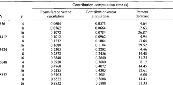
Table 3 illustrates the execution times of the distributed light contribution computations (Phase 4) during a single iteration of the parallel algorithm. The last column of Table 3 illustrates the percent decrease in the parallel execution time obtained by using the contribution vector circulation scheme instead of the form-factor vector circulation scheme. Note that the advantage of the contribution vector circulation scheme over the form-factor vector circulation scheme increases with increasing P as is expected.

Figure 6 illustrates the overall efficiency curves for the patch circulation approach. In Fig. 6, the efficiency curves are constructed using Eq. (18). Here, TSEQ and TPAR denote the execution time taken for the sequential algorithm and the parallel algorithm on P processors, respectively, to converge to the same tolerance value. Note that global shooting patch selection, loosely-coupled synchronous patch circulation with scattered decomposition, and contribution vector circulation schemes are used in Phases 1, 2 and 4, respectively, in order to obtain utmost parallel performance on the ring topology. As seen in Fig. 6, efficiency decreases with increasing P

for a fixed N in general. There are two main reasons for this decrease in the efficiency. The first one is the slight increase in the load imbalance of the parallel hemicube production phase with increasing P. The second, and the more crucial reason is the modification introduced to the original sequential algorithm

Table 3. Effect of the circulation scheme on the performance of the light contribution computation (Phase 4) Contribution computation time (s)

Form-factor vector Contributionvector Percent

N P circulation circulation decrease

856 4 0.0604 0.0576 4.64 8 0.0762 0.0664 12.63 16 0.1072 0.0784 26.87 1412 4 0.1012 0.0962 4.94 8 0.1232 0.1064 13.64 16 0.1680 0.1184 29.52 3424 4 0.2305 0.2202 4.46 8 0.2872 0.2456 14.48 16 0.3840 0.2640 31.25 5648 4 0.3920 0.3680 6.12 8 0.4760 0.4072 14.45 16 0.6385 0.4303 32.61 8352 4 0.5405 0.5081 6.00 8 0.6552 0.5608 14.41 16 0.8832 0.5888 33.33

(16)

322 C. Aykanat, T. K. Capm and B. Ozgii$ 06 0” 5 -= 05 E 04 O3 t 0.2 / 0 2000 4000 6000 8000 Number of patches (N)

Fig. 6. Overall efficiency.

for the sake of parallelization. As discussed earlier,

this modification increases the total number of

shooting patch selections required for convergence in comparison with the sequential algorithm. Figure 7, which illustrates the normalized efficiency values per single shooting patch computation, is presented

in order to confirm the latter reason. Figure 7

eliminates the effect of the increase in the number of shooting patch selections. Greater efficiency values in Fig. 7 than those in Fig. 6 reveal the performance degradation in the proposed parallel algorithm due to the increase in the number of shooting patch selections. As seen in Fig. 7, the efficiency of the parallel algorithm, per shooting patch computation, remains almost constant as is expected.

Table 4 illustrates the variation of the increase in the total number of shooting patch selections for different tolerance values and number of processors. In Table 4, 8% tolerance for convergence means that shooting patch selections continue until the total energy (i.e. the sum CL, ABiAi) reduces below E

percent of the initial energy (i.e. the initial sum). As seen in this table, the modification introduced for the

0.6 6 5 .= 0.5 E w 0.4 0.1 ‘- 0.0 - I / 0 2000 4000 6000 8000 Number of patches (N)

Fig. 7. Efficiency per shooting patch.

sake of efficient parallelization increases the total

number of shooting patch selections. The percent

increase in the total number of shooting patch

selections increases with increasing number of

processors as is expected. However, for a fixed

number of processors, this percent increase decreases with decreasing tolerance values. As seen in Table 4, the percent increase in the number of shooting patch selections remains below 12% for tolerence values

<60% for P< 128 processors. Hence, this paralleli-

zation scheme is highly recommended for medium

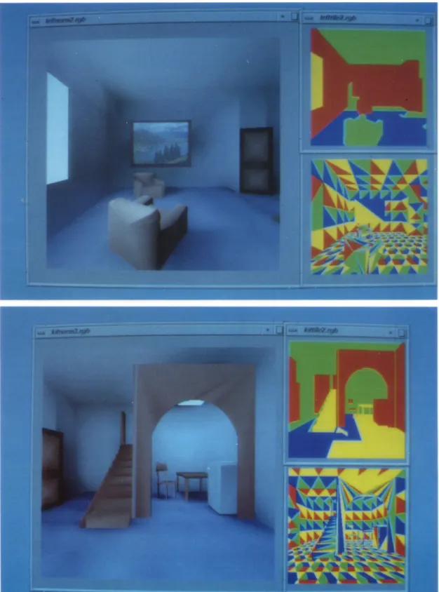
number of processors and medium tolerance values. Figure 8 illustrates two different views from the test scene data, and their tiled (upper right) and

scattered (lower right) decompositions. Different

colors (red, green, blue and yellow) denote patch

assignments to four processors in the respective

decompositions.

6. CONCLUSIONS

An efficient synchronous parallel progressive

radiosity algorithm based on patch data circulation

was proposed and discussed. The proposed scheme

Table 4. Total number of shooting patch selections of the parallel algorithm normalized with respect to those of the sequential algorithm

Final delta radiosity percentage (tolerance)

P 70 65 60 55 50 45 40 1 1.00 1.00 1 .oo 2 0.99 1.00 1 .oo 4 1.01 1.00 1.00 8 1.00 1.01 1 .oo 16 1.20 1.11 1.03 32 1.30 1.25 1.04 64 1.50 1.23 1.12 128 1.95 1.29 1.12 1.00 1 .oo 1 .oo 1 .oo 1.01 1.02 1 .Oh 1.11 1 .oo 1.00 1 .oo 1.00 1 .oo 1.00 1.00 1.01 1.01 1.01 1.02 1.03 1.05 1.05 1.11 1.08 1 .oo 1.00 1.00 1 .oo 1.01 1.02 1 .a4 1.07

(17)

Fig. 8. Two views from the test scene data with 3424 patches, and their tiled (upper right) and scattered (lower right) decompositions. Different colors in the decomposit-.on views denote processor assignments