Integrated flexible capacity and inventory management under flexible capacity uncertainty

(1)

INTEGRATED FLEXIBLE CAPACITY AND

INVENTORY MANAGEMENT UNDER

FLEXIBLE CAPACITY UNCERTAINTY

a thesis

submitted to the department of industrial engineering

and the institute of engineering and science

of bilkent university

in partial fulfillment of the requirements

for the degree of

master of science

By

Mehmet Fazıl Pa¸c

August, 2006

(2)

I certify that I have read this thesis and that in my opinion it is fully adequate, in scope and in quality, as a thesis for the degree of Master of Science.

Assist. Prof. Dr. Osman Alp (Supervisor)

Assist. Prof. Dr. Alper S¸en

Assist. Prof. Dr. Sedef Meral

Approved for the Institute of Engineering and Science:

Prof. Dr. Mehmet B. Baray

Director of the Institute Engineering and Science

(3)

ABSTRACT

INTEGRATED FLEXIBLE CAPACITY AND

INVENTORY MANAGEMENT UNDER FLEXIBLE

CAPACITY UNCERTAINTY

Mehmet Fazıl Pa¸c

M.S. in Industrial Engineering Supervisor: Assist. Prof. Dr. Osman Alp

August, 2006

In a manufacturing environment with volatile demand, inventory management can be coupled with dynamic capacity adjustments for handling the fluctuations more effectively. In this study we consider the integrated management of inven-tory and flexible capacity management under seasonal stochastic demand and uncertain labor supply. The capacity planning problem is investigated from the workforce planning perspective. We consider a manufacturing firm that can tem-porarily increase its production capacity by utilizing contingent workers from an external labor supply agency. The uncertainty of contingent capacity arises from the (un)availability of contingent workers, the pool size and the behavior of the labor supply agency. Using a dynamic programming approach, we formu-late an infinite horizon model determining the optimal levels of permanent and contracted capacity, in order to minimize the total cost of operations. Within the dynamic program, we determine the optimal operational capacity decisions, namely the size of contracted and contingent capacity to be utilized in each pe-riod. The characteristics of the optimal policies are analyzed under an infinite horizon setting. In addition we consider temporary labor contracts, that diminish the effects of supply uncertainty on the manufacturer, at a specific contracting cost. Our analysis shows that as the supply uncertainty and/or the expected cost of utilizing contingent workers increase, the value of temporary labor contracts also increase. In contrast increasing demand variability reduces the incentive of the manufacturer to own capacity and increases the utilization of contingent resources.

Keywords: Flexible Capacity, Capacity Management, Inventory, Production

Planning, Stochastic Dynamic Programming. iii

(4)

¨

OZET

TEDAR˙IK BEL˙IRS˙IZL˙I ˘

G˙I ALTINDA ES¸ZAMANLI

ESNEK KAPAS˙ITE VE ¨

URET˙IM PLANLAMA

Mehmet Fazıl Pa¸c

Endüstri Mühendisli˘gi, Yüksek Lisans Tez Yöneticisi: Yard. Do¸c. Dr. Osman Alp

A˘gustos, 2006

¨

Ureticiler talep dalgalanmalarına, envanter yönetimi ve e¸szamalı esnek kapa-site yönetimi ile etkin bir ¸sekilde kar¸sılık verebilirler. Bu ¸calı¸smada e¸szamanlı esnek kapasite ve envanter yönetimi, kapasite tedari˘gi ve mevsimsel talep belirsi-zli˘gi altında incelenmi¸stir. Kapasite planlama, i¸sgücü ba˘glamında ele alınmı¸stır.

¨

Uretim kapasitesi i¸s¸ci tedarik acentesinden ge¸cici i¸s¸ci alımıyla arttırılabilmektedir. Ge¸cici i¸s¸ci tedari˘gindeki belirsizlik, ortamdaki ge¸cici i¸s¸ci sayısından, i¸s¸ci tedarik acentesinin elindeki i¸s¸ci sayısından ve dönemsel kararlarından kaynaklanmak-tadır. Operasyonel maliyetler, dinamik programlama kullanılarak sonsuz plan-lama ¸cevreninde enaza indirgenmektedir. Bu ¸calı¸smada eniyi kapasite ve üretim politikalarının karakteristikleri incelenmi¸stir. Ge¸cici i¸s¸ci tedari˘gindeki belirsi-zlikten kaynaklanan etkileri azaltmak i¸cin tedarik¸ci acente ile i¸s¸ci kontratları yapılması önerilmektedir. Ge¸cici i¸s¸ci kullanımının beklenen maliyetinin, belir-sizlik ve/veya fiyattan dolayı artması durumunda i¸s¸ci kontratlarının de˘gerlendi˘gi gözlemlenmi¸stir. Buna kar¸sılık artan talep belirsizli˘ginin üreticiyi esnek kapasite kullanımına yöneltti˘gi ve kontratların de˘gerini azalttı˘gı görülmü¸stür.

Anahtar sözcükler : Esnek Kapasite, Kapasite Yönetimi, Envanter, ¨Uretim Plan-lama, Rassal Dinamik Programlama.

(5)

Acknowledgement

I would like to express my gratitude to Asst. Prof. Osman Alp for his guidance, patience and encouragement throughout this study.

I am indebted to Asst. Prof Sedef Meral and Asst. Prof. Alper S¸en for accepting to read and review this thesis and also for their valuable comments and suggestions.

I would also like to express my gratitude to TUBITAK for its support through-out my master’s study.

I am most thankful to G¨ulay for her support and her patience throughout this study.

I am deeply thankful to my family for believing in my work and supporting me. Special thanks to my brother Burak for encouraging me in coding.

Many thanks to all my friends in Bilkent IE, especially to Mehmet Mustafa Tanrıkulu for establishing Kaytarikcilar. Without the friendship all the burdens would be unbearable.

And to everyone, who trusted, helped and encouraged me throuhout my stud-ies.

(6)

List of Figures

5.1 Expected Inventory Level After Production-Uniform Uncertainty,

cp = 2.5, cc= 3.5, h = 1, b = 5 U = 10, Poisson Demand . . . . . 66

5.2 Optimal Capacity Position & Optimal Production vs Starting In-ventory Level - Uniform Uncertainty, cp = 2.5, cc = 3.5, h = 1,

b = 5 U = 10, Poisson Demand . . . . 67 5.3 Expected Inventory Level After Production vs Starting

Inventory-Normal Uncertainty, cp = 2.5, cc = 3.5, h = 1, b = 5 U = 10,

Poisson Demand . . . 68 5.4 Optimal Capacity Position vs Starting Inventory Level-Binomial

Uncertainty with Increasing Probability of Success, cp = 2.5, cc =

3.5, h = 1, b = 5 U = 10, Poisson Demand . . . . 69 5.5 Optimal Capacity Position vs Starting Inventory Level-Binomial

Uncertainty with Increasing Probability of Success, cp = 2.5, cc =

3.5, h = 1, b = 5 U = 10, Poisson Demand . . . . 70 5.6 Infinite Horizon Discounted Cost of Operations vs Capacity

Position-Binomial Uncertainty with Decreasing Probability of Suc-cess, cp = 2.5, cc= 3.5, h = 1, b = 5 U = 10, Poisson Demand . . 71

5.7 H(w|x = 0) vs Capacity Position-Binomial Uncertainty with In-creasing Probability of Success at High and Low Requests, cp =

2.5, cc= 3.5, h = 1, b = 5 U = 10, Poisson Demand . . . . 72

(10)

LIST OF FIGURES x

5.8 Optimal Capacity Position vs Starting Inventory Level-Binomial Uncertainty with Increasing Probability of Success at High and Low Requests, cp = 2.5, cc = 3.5, h = 1, b = 5 U = 10, Poisson

Demand . . . 73 5.9 Expected Inventory Level After Production vs Starting Inventory

Level-Binomial Uncertainty with Increasing Probability of Success at High and Low Requests, cp = 2.5, cc= 3.5, h = 1, b = 5 U = 10,

Poisson Demand . . . 74 5.10 Expected Inventory Level After Production vs Starting Inventory

Level-Binomial Uncertainty with Increasing Probability of Success at Moderate Requests, cp = 2.5, cc = 3.5, h = 1, b = 5 U = 10,

Poisson Demand . . . 75 5.11 Optimal Production vs Starting Inventory Level-Binomial

Uncer-tainty with Increasing Probability of Success at Moderate Re-quests, cp = 2.5, cc= 3.5, h = 1, b = 5 U = 10, Poisson Demand . 76

6.1 Periodic Production-Certain Supply vs Uniform Supply. U = 10,

V = 0, cc = 3.5, b = 50 . . . . 83

6.2 Value of Contracting vs Permanent Capacity Level-Uniform Sup-ply Uncertainty, Poisson Demand b = 50, cc= 3.5 . . . . 92

6.3 Relative Value of Contracting vs Permanent Capacity Level-Uniform Supply Uncertainty, Poisson Demand b = 50, cc= 3.5 . . 93

6.4 Value of Contracting vs Contracting Cost (ci) - Uniform Supply

Uncertainty, Poisson Demand b = 50, cc= 3.5 . . . . 94

6.5 Relative Value of Contracting vs Contracting Cost (ci) - Uniform

(11)

List of Tables

3.1 Summary of Notation . . . 21

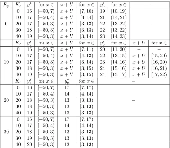
4.1 Computational Analysis-Parameter Set . . . 39 4.2 Effect of Kc on the optimal policy. U = 10, b = 50, cc = 3.5,

cp = 2.5 and h = 1. . . . 41

4.3 Effect of Kp on the optimal policy. b = 50, cc = 3.5, cp = 2.5 and

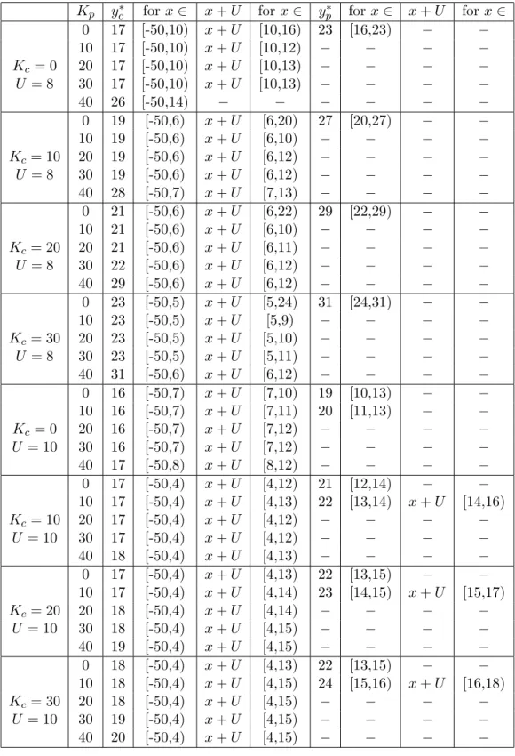
h = 1. . . . 42 4.4 Effect of U on the optimal policy. b = 8, cc= 3.5, cp = 2.5, Kc= 0,

Kp = 10 and h = 1. . . . 43

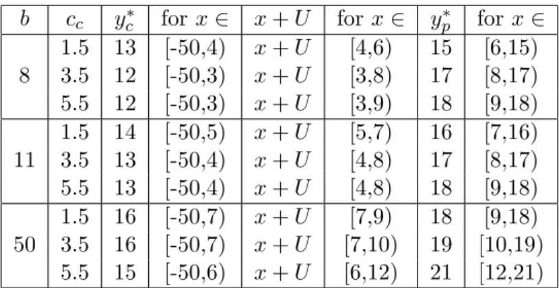
4.5 Effect of contingent labor cost and backordering cost on the opti-mal policy. U = 10, cp = 2.5, Kc= 0, Kp = 0 and h = 1. . . . 44

4.6 Effect of demand variability on the optimal policy. U = 10, cc =

5.5, cp = 2.5, Kc= 0, Kp = 0 and h = 1. . . . 45

6.1 Average Inventory Level and Average Production with Contingent Capacity. U = 6, V = 0 . . . . 80 6.2 Average Inventory Level and Average Production with Contracted

and Contingent Capacity. U = 10, V = 2, ci = 1.2 . . . . 82

(12)

LIST OF TABLES xii

6.3 Optimal Contracted Capacity Level (V∗_{)-Uniform Supply}

Uncer-tainty. . . 85 6.4 Optimal Contracted Capacity Level (V∗_{). U = 6, c}

c = 3.5 . . . . 86

6.5 Optimal Contracted Capacity Level (V∗_{). b = 50, c}

i = 0.6 . . . . 86

6.6 Effect of Backordering Cost on Optimal Contracted Capacity Level. Poisson Demand, cc= 3.5. . . . 87

6.7 Effect of Demand Uncertainty on Optimal Contracted Capacity Level. Poisson Demand, U = 6, cc= 3.5, b = 50. . . . 88

6.8 Effect of Contingent Labor Cost and Uncertainty on Owned Ca-pacity (U∗_{, V}∗_{). c}

p = 2.5, ci = 0.6, b = 50 . . . 90

6.9 Effect of Demand Variability on Owned Capacity. cc = 3.5, ci =

0.6. . . . 90 6.10 Effect of Backordering Cost on Owned Capacity. cp = 2.5, ci = 0.6. 91

6.11 Effect of Backordering Cost on V CC and %V CC. cc = 3.5, ci =

0.6. . . . 95 6.12 Effect of Contingent Labor Cost on Value of Contracting. b = 50,

ci = 0.6. . . . 96

6.13 Effect of Contingent Labor Uncertainty on Value of Contracting.

cc= 3.5, ci = 0.6. . . . 96

6.14 Effect of Demand Variability on the Value of Contracting. b = 50,

ci = 0.6. . . . 97

6.15 Heuristic Performance and Supply Uncertainty. (b = 5, 10, 15), (cc= 1.5, 3.5, 5.5) . . . . 99

6.16 Heuristic Performance (Average Gap) with Increasing Coefficient of Variation. Gamma Demand, b = 15, cc= 3.5 . . . . 99

(13)

LIST OF TABLES xiii

6.17 Heuristic Performance with Increasing Permanent plus Contracted Capacity. Uniform Supply Uncertainty, b = 15, cc= 3.5 . . . 100

6.18 Heuristic Performance with Increasing Permanent plus Contracted Capacity. Binomial Uncertainty with Increasing Probability of Success k = 20, b = 15, cc= 3.5 . . . 101

6.19 Heuristic Performance under different Backordering and Contin-gent Labor Costs. Uniform Supply Uncertainty, U = 6 . . . 102

(14)

Chapter 1 Introduction

Demand volatilities have significant impacts on companies in the manufactur-ing industry. Seasonal fluctuations in demand influence the production decisions of manufacturing companies. In make-to-stock environments, a conventional ap-proach is holding safety stocks for coping with uncertainties in demand. An alter-native approach could be switching manufacturing lines between seasonal prod-ucts prior to seasonal demand peaks. Under the existence of non-stationarities in demand, dynamic capacity adjustments arise as an effective tool in addition to these approaches. Manufacturing companies may increase their production capacity temporarily by acquiring external capacity resources (e.g. outsourcing, short term machinery leasing, hiring temporary workers). Effective utilization of such resources may result in increased demand responsiveness and reduced op-erational costs. However external capacity may not always be available at the desired amount and/or quality in the environment. Therefore the manufacturer has to consider the effect of uncertainty in the supply of external capacity, when making the production plan. In this study, we consider the integrated planning of production, inventory and flexible capacity under demand and external capacity supply uncertainties.

(15)

CHAPTER 1. INTRODUCTION 2

Capacity flexibility within the context of this study is the ability of the man-ufacturer to temporarily increase the production capacity with the usage of ex-ternal resources. The problem under consideration focuses on labor intensive production environments, therefore capacity will be analyzed under the work-force context. Capacity can be defined as the maximum amount of production that can be achieved by utilizing internal and external resources. Production capacity of the firm can be classified under two main categories: Permanent ca-pacity and temporary caca-pacity. Permanent caca-pacity can be considered as the maximum amount of production that can be achieved by the company’s owned workforce, which is under the steady payroll. External capacity resources in our context are the contingent workers that are temporarily acquired from an external labor supply agency (ELSA). External labor supply agencies provide contingent workers to firms, from its own pool of workers or by finding temporary workers from the environment. Contingent worker requests of the manufacturer may not be met in full terms by the ELSA due to two main reasons. The first reason is that the ELSA may not be capable of meeting the manufacturer’s request due to the lack of availability or skill of temporary workers. In the second case however, the ELSA may not be willing to meet the request of the manufacturer consid-ering possible better alternatives in the market. In both cases the contingent labor request of the manufacturer may be totally unmet or partially fulfilled. A labor supply contract that is signed between a manufacturer and an ELSA is a possible way to alleviate the impact of labor supply uncertainty on the manu-facturer. On the other hand, such a contract would bring guaranteed sales to the ELSA. There may exist a variety of labor contracts. In our setting the labor supply contract between the manufacturer and the ELSA is specified as follows. The manufacturer pays a specific fee each period per contracted worker and the ELSA provides contracted workers to the manufacturer with certainty with an additional fee per worker requested. Under this setting, the notion of contracting that we present becomes similar to option contracting. The cost of contracting is analogous to the reservation cost and the utilization cost is analogous to the exercise cost of option contracts. The manufacturer may still request contingent workers in addition to the contracted workers, but such workers are subject to supply uncertainty. Under this setting, we classify external capacity resources

(16)

under two categories: Contracted workers and contingent workers.

In this study we focus on designing labor supply contracts as well as the si-multaneous management of capacity, production and inventory under a periodic review make-to-stock environment with non-stationary stochastic demand and uncertain labor supply. The design of the contract includes the determination of the number of contracted workers and the fees paid for those workers. Permanent capacity levels of companies are not adjusted frequently. In general a strategic decision on the permanent capacity level is given at the beginning of the plan-ning horizon and it is not changed until a significant shift in the environment. In our problem permanent and contracted capacity levels are determined at the beginning and fixed throughout the planning horizon. Nevertheless, we analyze the problem under an infinite planning horizon setting in order to reflect the long term benefits of integrated capacity and production management.

Demand seasonality is one of the main driving forces behind dynamic capacity adjustments. Seasonality trends affect a major portion of the manufacturing and service industries. To give a brief description, seasonality can be defined as the source of predictable and uncontrollable variations in demand, which occur on a recurrent basis. Seasonality has many causes. Among the most general ones are natural causes such as weather, periodic annual government actions such as taxation; new product introductions especially in automotive and electronics in-dustries; and seasonal patterns resulting in periodic peaks such as the Christmas season. As seen in the automotive and electronics examples sometimes industries create their own seasonality. Among the periodic trigger factors are annual trade shows and new product releases.

Companies facing seasonal fluctuations in demand generally use the approach of building up inventory for meeting peak demands, however, keeping excessive inventory, especially under the requirement of high service levels, may be too costly. On the other hand, under the presence of apparent seasonality, utilizing

(17)

flexible capacity may become a better approach. Determining the production capacity is generally considered as a strategic or tactical level decision. However, under the presence of capacity flexibility, it is a crucial decision at the operational level as well. After the determination of the permanent production capacity at the tactical level, the responsibility of the operational level is the management of capacity by utilizing external resources when necessary.

Dynamic adjustments of the permanent capacity, such as hiring or firing, are generally too costly. Besides the social and motivational effects, such adjust-ments, tend to have a negative effects on the efficiency of workers. When making the capacity decisions, a company must be aware of the long-run pattern of fluc-tuations and must set the permanent level of capacity accordingly. Setting the permanent capacity levels too high may result in excessive labor costs while low levels of permanent capacity may result in backordering or additional capacity acquisition costs. Under an unstable market, the strategic decision of determin-ing the permanent capacity level is generally difficult when considerdetermin-ing the long period of circulation. However, when the pattern of seasonality and the stabil-ity of the market is known, permanent capacstabil-ity levels can be set more effectively considering flexible capacity management. While such downright planning of per-manent and external capacity levels may result in major reductions in long-run operational costs, even the operational decision of determining the appropriate temporary capacity level alone yields significant benefits. Presence of a tight competition in the aforementioned environments increases the incentive of using flexible capacity to cut down operational costs. Especially when the inventory holding and/or backordering costs are high, the firm may rely on temporary ca-pacity for meeting the demand.

Considering the capacity as the workforce level, we focus on the utilization of flexible workforce as contingent (contracted or temporary) capacity. Throughout the world, the usage of temporary workforce drastically increased from the late 80’s through the mid 90’s [6]. US Bureau of Labor Statistics indicates that in February 2005 there were 10.3 million independent contractors (7.4 percent of

(18)

total employment), 2.5 million on-call workers (1.8 percent of total employment), 1.2 million temporary help agency workers (0.9 percent of total employment), and 813,000 workers provided by contract firms (0.6 percent of total employment) in USA [24]. Aside from the workers with alternative work arrangements as indi-cated above, contingent workers (temporary jobs) accounted for 4.1 percent of the total US employment. As another example, 6.6 percent of the active labor force of the Netherlands was composed of flexible workers (temporary, standby, replacement and others) in 2003 [5]. In March 2006, 7.9 percent of the active labor force in Turkey was composed of contingent workers [32].

Temporary workers can be hired anytime and they are generally paid for labor hours. Experience shows that it takes as short as 1-2 days to receive temporary workers from external resources, such as labor supply agencies. The wage rate for temporary workers tend to be lower than that of their permanent counterparts however their costs to the hiring firm are generally higher. Nevertheless we do not confine ourselves to such constraint in our analysis. Productivity of tempo-rary workers may vary for industries requiring different levels of skill. However for jobs with little or no skill requirement, temporary workers may not cause a significant reduction in productivity.

Availability of temporary workers is a major concern when the manufacturer relies on external capacity for production. A manufacturer may not always ac-quire contingent workers in the desired quantity and/or quality. The underlying reasons for availability uncertainty of temporary workers can be as follows. In a tightly competitive environment finding the desired quantity of temporary work-ers with the required set of skills may not be possible as the demand for skilled labor ascends. On the other hand, a labor supply agency may consider more than one alternative at a time, in contemplation of maximizing its benefits. In this case a manufacturer’s request for temporary workers may be rejected if there exists a better alternative for the ELSA. Labor supplier’s behavior and the avail-able worker pool size may induce an uncertainty for the availability of temporary workers. While an ELSA with a large pool size may avoid small sized requests,

(19)

another ELSA with a limited pool size may motivate small sized requests by offering higher availability rates. Another important factor affecting the avail-ability of temporary workers is the labor demand in the market. In a season with intense labor demand it is difficult to find temporary workers with the required skill level in the desired quantities. The skill level required by the manufacturer is also a factor causing uncertainty in temporary workforce availability. The labor supply agency may not be capable of finding workers with the required skill in the desired quantity. In addition, the delivery lead time and the timing of the request can be considered as a source of availability uncertainty. An ELSA may not always be quick enough in responding to a firm’s request.

Contracting with the ELSA for temporary workers is a good solution for ab-rogating the effect of availability uncertainty. Contracted workers are available to the manufacturer whenever requested. Contracting may increase costs, as the manufacturer pays a specific fee to the ELSA even if the contracted workers are not utilized. But under appropriate cost rates, it is an attractive tool for dimin-ishing the effects of availability uncertainty. In this study we investigate different settings to find out the cases where the manufacturer is better off with contract-ing. We also determine the optimal contract sizes under such cases.

In this study we analyze the problem of determining the capacity levels simul-taneously with the production decision within the aforementioned environment. We find the optimal operational parameters with an infinite horizon dynamic program under discounted cost criterion. The problem is analyzed under differ-ent supply uncertainty structures. The structure of the availability uncertainty is dependent on the amount of contingent capacity requested by the manufac-turer. The uncertainty structures include the cases where the availability rate is increasing or decreasing in the number of contingent workers requested. The characteristics of the optimal policy are discussed for different settings under dif-ferent supply uncertainty types. We also consider a special case of the problem where there is no supply uncertainty. We show that the finite horizon results of the problem (as discussed by Tan and Alp [31]) extend to infinite horizon. An

(20)

important result that we provide in this study is the value of contracts. In cases where contracting temporary workers is beneficial for the manufacturer, we elab-orate on the value of the contract by the savings gained. Computational analysis shows that contracting saves up-to 12 percent of the expected total cost in the experimental settings considered. Finally, a comparison of the cases with and without the presence of labor supply uncertainty is made. We illustrate the effect of supply uncertainty on the contingent capacity usage.

The rest of the thesis is organized as follows. In Chapter 2, we provide an extensive review of the related literature. In Chapter 3 we introduce our model and the supply uncertainty structures. In Chapter 4, a special case of the problem, where contingent labor is available with certainty is analyzed in an infinite horizon context. In Chapter 5, we analyze the problem and provide the characteristics of the optimal policy. Optimal permanent and contracted capacity levels, value of optimal contracts, comparison of the optimal policy with a heuristic policy and the effect of labor supply uncertainty is provided by the numerical analysis in Chapter 6. Finally a summary of results, conclusions and possible extensions are given in Chapter 7.

(21)

Chapter 2 Literature Review

Capacitated production/inventory problems and capacity/workforce planning problems have been extensively studied in literature separately. However a com-bined dynamic approach is not yet thoroughly analyzed. The problem under con-sideration focuses on the simultaneous planning of capacity and production under the presence of demand and capacity uncertainty. Therefore it has strong interac-tions with the following fields: (i) integrated production/capacity planning, (ii) workforce planning and flexibility, (iii) capacitated production/inventory plan-ning and (iv) production/inventory planplan-ning with random capacity/yield. Here we provide a brief summary of the most related works in these fields and discuss their similarities and differences with our problem.

Capacity planning has been analyzed extensively in all levels of decision mak-ing. While the earlier works generally focus on strategic and tactical perspective, recent studies integrate an operational approach. An in depth review on strategic capacity management is provided by Van Mieghem [22]. The paper presents the fundamentals of the formulation and solution of major capacity planning prob-lems, concerning the size, type and timing issues in an environment with demand and/or capacity uncertainty. The author also focuses on the recent studies focus-ing on multiple capacity types.

(22)

CHAPTER 2. LITERATURE REVIEW 9

Atamturk and Hochbaum [4] focus on an integrated capacity and production planning problem under a non-stationary deterministic demand setting. Authors exploit the trade-offs between capacity expansions, subcontracting and inventory holding. The study is precursory in integrating the cross-impacts of decisions af-fected by capacity expansions. We investigate a similar problem under stochastic demand and with flexible capacity management instead of capacity expansions. Angelus and Porteus [2] concentrate on a simultaneous capacity and production planning problem for short life-cycle products, under stochastically increasing and then decreasing demand structure. The study investigates capacity expansions as well as contractions at exogenously determined prices. Target interval policy is shown to be optimal in both cases, with or without inventory carry-over. Target interval policy requires the smallest possible change in the capacity level in each period in order to bring the available level into the target interval of that period. In case of no inventory carry-over, authors provide a detailed characterization of the target intervals. For the case of inventory carry-over a general result is established and then capacity and inventory are shown to be economic substi-tutes. Authors indicate that capacity target intervals are decreasing in the initial inventory level and the optimal base stock levels decrease in the capacity level. The notion of dynamic capacity adjustments and integrated production planning provided in this study is comparable to that of our model. One major distinction between this study and our work is that, it considers periodic hiring and firing decisions for adjusting capacity, whereas we consider utilizing external capacity resources for a fixed permanent capacity level.

Dallaert and de Kok [8] investigate the integrated capacity and production planning problem under a more flexible capacity setting. In their study, capacity is composed of long-term contract workers and temporary workers. Authors ana-lyze the capacity and production planning problem in a decoupled approach and an integrated approach. In the decoupled approach, separate resource and pro-duction decisions are made in the following order. First the order up-to levels and production decisions are made and then the levels of regular and temporary work-force are determined accordingly. In the integrated approach however, decisions

(23)

are made simultaneously. It is shown that the integrated approach outperforms the decoupled approach. The model of flexible capacity management used in this model is similar to our setting. However this study initially solves the inventory problem and accordingly determines the capacity levels, whereas we consider an integrated approach, considering the uncertainty in temporary production capac-ity. Hu et al. [18] investigate the problem of minimizing the long-run average cost of holding inventory and/or purchasing extra capacity under demand fluc-tuations. The study considers a fixed permanent production capacity, which can be temporarily increased by utilizing contingent capacity. Authors model the problem on a continuous time framework under a Markov modulated high-low demand rates. It is shown that the optimal policy is of hedging point type, where two hedging levels are associated with each discrete state of the system. The positive hedging level corresponds to the inventory target, while the negative hedging level corresponds to the backlog level below which extra capacity should be purchased. In a similar problem, Tan and Gershwin [30] study production and subcontracting strategies with limited production capacity and fluctuating de-mand. The problem under investigation considers lead time sensitive customers, who choose not to order for excessive lead times. The firm has a set of sub-contractors with different capacity levels in order to supplement the production capacity. Authors derive a hedging type policy, namely the feedback policy, for determining the production rate and the rate at which subcontractors should be requested. The model presented in this study has similarities with the system that we consider, however we investigate the problem under periodic review in an environment with supply uncertainty. Yang et al. [36] deal with the optimal production-inventory-outsourcing policy for a firm with Markovian production capacity facing independent stochastic demand and the option of outsourcing. The model does not associate a fixed cost for production but outsourcing has a fixed cost. The decision maker in this model decides on the amount to be outsourced for the next period after observing the realized internal capacity and the demand. Therefore the problem does not consider a simultaneous planning of production/capacity. Authors derive simple optimal policy forms under rea-sonable assumptions. For stochastically monotone Markovian capacity, policy parameters are shown to be decreasing in the firm’s current capacity level under

(24)

some basic conditions. The authors show that the results hold for infinite horizon and undiscounted-cost cases and derive the conditions under which outsourcing is more valuable. The model in this problem offers outsourcing as a tool to reduce the effect uncertain internal capacity, on the other hand in our model we present uncertain capacity outsourcing as a tool for coping with demand fluctuations.

Tan and Alp [31] consider the management of flexible capacity, inventory and the determination of permanent capacity level under non-stationary stochastic de-mand in a finite planning horizon. This study constitutes the basis of our study. The model analyzed is based on production system where contingent workers are utilized on top of the permanent capacity, whenever required. The study con-siders cases with and without setup costs for initiating production and utilizing contingent capacity. Authors analyze the characteristics of the optimal policy for the integrated capacity/production planning problem and evaluate the value of utilizing flexible capacity under different settings. A state dependent order up-to type policy is shown to be optimal. Optimal order up-to points are shown to be non-decreasing in the initial inventory position. The study derives two critical points, one for production with permanent capacity and the other for production with permanent plus contingent capacity, which are shown to be non-increasing in the number of periods remaining. Our study is an extension of this study. We consider the availability uncertainty of contingent workers and introduce con-tracted workers as a source for diminishing the effects of uncertainty. Alp and Tan [1] consider the tactical planning of capacity under capacity flexibility in a periodic review make-to-stock environment with stochastic demand. Capacity flexibility in this model is provided by contingent workers which can be acquired whenever requested. The study derives optimal production parameters and the tactical capacity level and derives the value of flexibility under various conditions.

In the field of workforce planning and flexibility, Holt et al. [17] pioneer the research with the seminal work that presents models that analyze the trade-off between keeping large sized permanent workforce levels and frequent workforce level modifications for satisfying peak season demands under demand fluctuations.

(25)

This study is a milestone in introducing the notion of flexible capacity manage-ment. The model of flexible capacity management that we provide is an extension of this model with demand and supply uncertainty. Wild and Schneeweiss [35] analyze manpower capacity planning with a hierarchical approach. Optimization of the hierarchical model presented in the paper is done by using a stochastic dynamic program. The paper demonstrates the simultaneous application of vari-ation of monthly working time, overtime, utilizing contingent workers and leasing of work force and compares their performances.

Milner and Pinker [23] analyze the design of labor supply contracts between firms and external labor supply agencies (ELSA). The contract under their study includes long term contracted workers and temporary workers, that will be pro-vided to the firm which already has a specific level of permanent capacity. Au-thors analyze the problem in a single period environment, for both parties in-volved (firm and the ELSA). The study involves an uncertainty for temporary (non-contracted) workers provided by the ELSA under two different settings: Productivity uncertainty and availability uncertainty. Therefore the effect of un-certainty on contracts is analyzed under two different perspectives. In case of productivity uncertainty equilibrium contracts that coordinate both the firm and the ELSA in an optimal way exist. On the other hand under availability uncer-tainty, it is shown that it is not possible to construct optimal contracts. However there is still a wide region of parameters, where both parties are better-off with a contract. The paper investigates such set of parameters and trade-offs that should be considered in workforce contract negotiations. The model of flexible capacity management that we use is the same with the model introduced in this study. However we consider a multi-period setting where inventory carrying and backordering are allowed. Pinker and Larson [25], in a similar setting, focus on the determination of regular and contingent worker pool sizes for service indus-tries from a more tactical perspective. The operational control parameters are determined with a stochastic dynamic programming approach, and the tactical level of permanent and temporary capacity are determined accordingly. In their study regular workers are defined as workers with fixed schedules, who can also

(26)

work overtime. Contingent workers on the other hand have flexible working hours specified by the contract over the finite planning horizon. The model represents a variety of contracts such as temporary workers, on-call workers with guaranteed minimum pay, and compensatory time arrangements. The model is formulated in order to minimize the expected labor and backlogging costs by optimal plan-ning of regular and contingent worker levels. The problem includes the optimal planning of operational staffing decisions, such as overtime and capacity utiliza-tion. The study also reflects the effects of information timing on the benefits of flexibility. This study considers a multi-period flexible capacity planning problem from the service perspective. The decision of overtime and the number of contin-gent workers to be utilized is given according to the workload in the system. We study a similar flexible capacity management problem from the manufacturing perspective, where backordering and inventory carryover is allowed. The pool of contingent workers mentioned in this study is similar to the concept of contracted workers in our study. One major distinction is that we consider the availability of additional contingent workers with supply uncertainty.

In the field of capacitated inventory/production management, Federgruen and Zipkin [12] provide a fundamental analysis under stochastic demand. The study shows the optimality of base stock type policies when there exists no setup costs of production. Kapuscinski and Tayur [20] extend the results of Federgruen and Zipkin [12] by proving the optimality of the base stock policy under finite horizon, discounted infinite horizon and infinite horizon average cases for general Marko-vian, periodic demand. The authors use a simulation based technique to compute the optimal parameters and indicate several properties of the optimal policy. Gal-lego and Scheller-Wolf [13] consider the same problem under the existence of fixed order costs. By generalizing the K-convexity as CK-convexity, authors provide a partial characterization of the optimal policy. The optimal policy is shown to have an (s,S)-like structure. To characterize the optimal policy, the parameter space is divided into four regions. While in two of these regions the optimal policy is completely characterized, in the other two, it is partially specified. The study suggests the existence of a simpler optimal policy structure, however the

(27)

authors indicate that under specific parameter sets there still could be regions between the two critical points s and s0_{, where starting and stopping ordering}

can be optimal in succession. The problem considered in this study is a special case of our problem, where no contingent workers are available. In Chapter 5, we analyze the special case of our problem where the contingent workers are available with certainty. Our analysis shows that the optimal policy changes for different regions of starting inventory level as in Gallego and Scheller-Wolf [13], however the characteristics of the optimal policy are different.

When we consider the field of production/inventory planning under random capacity/yield, Silver [29] pioneers the research with the analysis of optimal order quantities when the arriving quantities are random under deterministic demand. The study extends the economic order quantity formulation with supply uncer-tainty in two different modes; in the initial case the variation of the quantity received is independent of the quantity ordered Q, whereas in the second it is dependent on Q. The study indicates that the optimal order quantity depends only on the standard deviation of the amount received. Yano and Lee [37] review the literature of lot sizing under random production or procurement yields. The study presents various methods in modeling of cost, yield uncertainty and perfor-mance in the context of systems with random yields. The literature investigated in this study considers a single source for production/procurement which is sub-ject to a random upper limit (capacity), where the decision under question is the order quantity. Authors investigate the structural results of the previous works, indicate their shortcomings and provide directions for future research.

Ehrhardt and Taube [9] focus on the single period inventory model with ran-dom replenishment quantities and ranran-dom demand. The replenishment quantity is considered as a random function of the amount ordered. The study charac-terizes the structure of optimal policies for linear ordering costs. For the case of no setup costs the optimal policy is shown to be of base stock type. Under the existence of setup costs, authors indicate that the optimal policy is of (s, S) type. The uncertainty model that we develop for the contingent workers is analogous to

(28)

the uncertainty model used for the replenishment quantities in this study. Wang and Gerchak [33] consider continuous review inventory control under variable capacity. The study analyzes the effects of variable capacity on optimal lot siz-ing in continuous review environments. Authors consider two models; the basic EOQ model and the order quantity/reorder point model with backlogging. For both cases, the optimality conditions for generally distributed variable capacity are presented. The analysis indicates that the optimal order quantities for both models and the optimal reorder point for the second model, are greater than those without variable capacity. The study also provides effective procedures for finding optimal solution for exponentially distributed variable capacity. Erdem and Ozekici [11] consider a single item inventory model in a randomly changing environment under periodic review. Model parameters are specified by the state of the environment which is determined by a time-homogenous Markov chain. Random yield is due to the random capacity of the vendor. The problem is an-alyzed in single period, multiple periods and infinite horizon. In all cases it is shown that the optimal policy is an order up-to level policy, which is dependent on the state of the environment. Their analysis show that the order up-to levels are identical with the results of the certain yield (infinite supply) case in the sin-gle period. However the multi-period and infinite horizon results show that the presence of an uncertain yield results in order up-to levels greater than or equal to that of the model with certainty.

Ciarallo et. al. [7] analyze the optimality of extended myopic policies under uncertain capacity and uncertain demand in a periodic review production plan-ning system. In the single period analysis, it is shown that the random capacity does not affect the optimal policy but results in a unimodal, non-convex cost function. Optimal policies for single period are drawn by classical convexity ar-guments due to the unimodality. In the multi-period case despite the non-convex cost function optimal policies are shown to be of order up-to type for finite and infinite horizon settings. The results indicate that the optimal policy and the critical numbers depend on the distribution of capacity uncertainty. Authors in-dicate the benefit of extended myopic policies under the consideration of review

(29)

period of uncertain length. The uncertainty of production capacity specified in this study is analogous to that of our model. However in our study, production capacity is also considered as a decision variable, and it can be increased by uti-lizing contracted and contingent workers. On the other hand this study considers the production level as a decision variable which is constrained by the uncer-tain production capacity. Another important distinction is that we consider the availability uncertainty only for contingent workers and assume that the owned production capacity is always fully available, whereas this study considers the uncertainty of the whole production capacity. Iida [19] studies a non-stationary periodic review dynamic production inventory model with uncertain production capacity and uncertain demand. The author derives upper and lower bounds for the optimal order up-to levels and shows that the upper and lower bounds of the finite horizon problem converge in the infinite horizon problem. This study is analogous to our work as it considers production planning under uncertain capacity and uncertain non-stationary demand. However in our study we con-sider production capacity as a decision variable, whereas this study concon-siders the uncertainty within the owned capacity of the firm and decides only on the pro-duction level.

Wang and Gerchak [34] combine the concepts of variable capacity and random yield in a periodic review production planning model with uncertain demand. The cost minimization problem under investigation is solved by a stochastic dynamic program. Authors prove that the finite horizon objective function is quasi-convex and the resulting optimal policy is a single critical point policy. The model pro-vided in their study is a generalization of a previous model by Henig and Gerchak [16] which only considers random yields. Results of this study indicate that the finite horizon solutions converge to infinite horizon results. The study indicates that when both random yield and variable capacity are present at the system the optimal policy is of reorder point type, whereas with the presence of variable capacity alone it is of order-up-to type. Erdem et. al. [10] focus on a continu-ous review inventory system with deterministic demand and multiple suppliers with variable capacities. In this model the quantities received from suppliers are

(30)

equal to the ordered quantities if the realized capacities are sufficient, otherwise the firm receives the maximum amount that the realized capacity provides. The study aims to specify the optimal order quantities while diversifying the risk of shortage, by utilizing n suppliers. Each supplier in this model has a specific lead time and a continuous distribution of capacity. Gullu [14] focuses on base stock policies for production/inventory problems with uncertain capacity levels. The periodic review model differs from previous research in the sense that it gives a discrete time environment. Post production inventory level is either the quantity ordered (if the capacity permits) or the inventory level before production plus the full available capacity. The system is analyzed under expected average cost per period criterion. The system operates under a stationary modified base stock policy. The main contribution of this study is that it establishes an analogy be-tween the class of base stock production/inventory policies that operate under demand/capacity uncertainty and G/G/1 queues and their associated random walks. The problem investigated in this study has a strong resemblance with our model in essence, however the definitions of capacity result in a fundamental distinction. In our study we define the production capacity as the total of perma-nent, contracted and contingent capacity, and introduce the number of contracted and contingent workers to be utilized as a decision variable. The uncertainty in the production capacity in our study arises from the uncertainty of the contin-gent capacity. On the other hand Gullu [14] considers the production level under variable production capacity as the decision.

Kouvelis and Milner [21] analyze the joint effects of demand and supply un-certainty on capacity and outsourcing decisions in multi-stage supply chains. Au-thors analyze the investment of a firm on the two stages of a supply chain, in which the first stage is responsible of the core activities of the firm while the second is responsible for the non-core activities. The objective is maximizing the multi-period discounted profit. The study discusses the effect of non-stationary stochastic demand on the outsourcing decisions and the effect of non-stationary supply, due to the market demand, on the capacity decisions. Characterization of the single period and the multi-period optimal capacity investment decisions

(31)

have been provided and the effects of changes in supply and demand uncertainty on the extent of outsourcing have been analyzed. The analysis shows that as the supply uncertainty increases capacity investments increase. On the other hand in-creasing demand uncertainty results in an increase on the reliance to outsourcing. Results indicate that if the demand is independent and identically distributed for all periods then it is not optimal to modify capacity after the first period. The model considered in this study has similarities with our model, however the ca-pacity investments considered in this study are less dynamic, considering that the changes are made in the beginning of critical periods as expansions with a fixed cost paid only at the time of investment. Also the outsourcing option presented in this model differs from our decision of contingent capacity.

Gullu et. al. [15] analyze a periodic review, single-item inventory model un-der supply uncertainty. The authors model the uncertainty in supply using a three-point probability mass function; supply is either fully available, partially available or unavailable. The study shows the optimality of order up-to type policies by using a stochastic dynamic programming formulation. Schmitt and Snyder [28] examine a model with supply uncertainty from the outsourcing per-spective. In their model supply is subject to regular variance as well as complete disruptions. Authors analyze the model under two different cases. In the initial case the unreliable supplier is the only option, whereas in the second case there exists a second reliable supplier with a higher cost rate. The study determines optimal order and reserve quantities. The case with a second reliable supplier is similar to our model, where we have uncertain contingent workers and cer-tain owned capacity (permanent and contracted workers). Both studies provide important information on the trade-off between supply uncertainty and the cost of capacity/supply certainty. However our work differs from their study, as we plan the flexible workforce and determine the production after realizing the ca-pacity. Arikan et. al. [3] provide an analysis of a periodic review capacitated inventory system with supply uncertainty where advance demand information is available. Authors assume three different supply processes, namely all or noth-ing type, partial availability and binomial availability. The all or nothnoth-ing type

(32)

contingent labor supply uncertainty model that we analyze reduces to the all or nothing supply uncertainty problem modeled in this study, as capacity is fully utilized in our optimal production policy. A major distinction of our work from this study is that we determine the optimal production quantity after realizing the capacity, therefore requested capacity is not always fully utilized, whereas in this study the realized amount of supply is always used. In addition we consider the utilization of contracted workers for reducing the effects of supply uncertainty.

All in all, the problem that we analyze is closely related with the aforemen-tioned fields. We analyze the integrated capacity and production planning prob-lem from a workforce planning perspective. The studies in the field of flexible capacity management up to now have assumed that there is an ample supply of external capacity that can be acquired at a specific cost. There exists recent studies considering uncertainty of contingent workers, however the problem of flexible capacity management has not yet been analyzed with labor supply un-certainty in a production environment, where inventory carryover is allowed. Our major contribution to the literature is that we introduce the supply uncertainty of contingent workers in a production environment and illustrate the trade-off between holding inventory and utilizing external capacity. Another key contribu-tion of our study is that we introduce temporary worker contracts for diminishing the effects of uncertainty. Under the presence of contracts, we analyze the cost of contingent capacity uncertainty and determine the amount that the manufac-turer is willing to pay to abrogate it. On the other hand, in the literature of production/inventory management under random yield there is a single decision, which is the production/order quantity. We introduce capacity and production decisions separately but plan the levels simultaneously.

(33)

Chapter 3 Model Formulation

In this section, we provide a dynamic programming formulation that can be used to solve the integrated capacity and inventory management problem under con-sideration. We first present our basic definitions, assumptions and settings.

We define capacity position w as the total amount of capacity requested by the manufacturer. Capacity level is defined as the production capacity observed after the uncertainty is resolved, i.e. after the realization of the contingent capacity (if any) is observed. If the capacity position is less than or equal to the permanent production capacity plus the contracted capacity (w ≤ U + V ), the capacity level is equal to the capacity position. On the other hand, if w > U + V , then the capacity level is a number between U + V and w. The permanent and contracted capacity levels are fixed and fully available throughout the planning horizon, but are decision variables to be determined at the beginning of the planning horizon. The unmet demand is fully backlogged. The costs under consideration are in-ventory holding and backordering costs, and unit costs of permanent, contracted and contingent capacity, which are all non-negative. We assume that there are no shortages of raw material and the lead time of production and acquiring external capacity can be neglected. There are no fixed costs for initiating production and no material related costs are considered in the model. The notation is summa-rized in Table 3.1. Further explanation of notation will be provided as need arises.

(34)

CHAPTER 3. MODEL FORMULATION 21

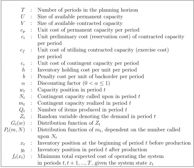
Table 3.1: Summary of Notation

T : Number of periods in the planning horizon

U : Size of available permanent capacity

V : Size of available contracted capacity

cp : Unit cost of permanent capacity per period

ci : Unit preliminary cost (reservation cost) of contracted capacity

per period

cf : Unit cost of utilizing contracted capacity (exercise cost)

per period

cc : Unit cost of contingent capacity per period

h : Inventory holding cost per unit per period b : Penalty cost per unit of backorder per period α : Discounting factor (0 < α ≤ 1)

wt : Capacity position in period t

Nt : Contingent capacity called upon in period t

mt : Contingent capacity realized in period t

Qt : Number of items produced in period t

Zt : Random variable denoting the demand in period t

Gt(w) : Distribution function of Zt

Pt(m, N ) : Distribution function of mt, dependent on the number called

upon Nt

xt : Inventory position at the beginning of period t before production

yt : Inventory position in period t after production

ft(xt) : Minimum total expected cost of operating the system

in periods t, t + 1, ..., T , given the system state xt

Throughout our analysis, we consider linear costs of capacity. The cost of permanent capacity is independent of the production quantity and paid each pe-riod even if there is no production. The unit cost of permanent capacity is cp

per period. Therefore the total permanent capacity cost for a workforce of size

U is cp∗ U per period. In the particular contract type that we consider the unit

cost of contracted workers (c0

w) is composed of two components; ci and cf, where

c0

i + c0f = c0w. c0i is the amount of money paid for each contracted worker at the

start of every period, independent of their utilization. This cost component cor-responds to the cost of keeping contracted workers. There is also an additional cost component c0

f, which is paid for each contracted worker utilized in

(35)

by a permanent worker in a period in order to bring production and capacity into a line. The initial cost of contracted workers and the cost of production for contracted capacity and contingent capacity are also defined in the same unit ba-sis. Considering that productivity rates of permanent, contracted and contingent workers differ in nature, let λc and λv be the productivity rates of a contingent

worker and a contracted worker, respectively. The model works for all values of

λc and λv, however we consider 0 < λc ≤ λv ≤ λp = 1 as permanent workers

are expected to be the most productive, whereas contingent workers are expected to be the least. Recalling that c0

i and c0f are the initial cost and the utilization

cost of a contracted worker respectively, the unit initial and utilization costs of a contracted worker can be written as ci = c0i/λv and cf = c0f/λv, respectively,

assuming that the productivity remains identical among the contracted workers. Similarly the unit cost of production for a contingent worker can be written as

cc = c0c/λc, where c0c is the unit cost of a contingent worker. The total initial

cost of contracted workers of contracted capacity is equal to ci ∗ V if the total

contracted capacity is equivalent to V productive units. From now on permanent equivalent units will be considered for contracted and temporary workers. In particular N contracted/temporary workers will produce N units of product in a period.

The amount of contingent capacity received, m is distributed by P (m, N ), which depends on the number of contingent workers requested N. The firm can receive at most N and at least zero contingent workers depending on the type of the corresponding probability distribution. The total cost of contingent capacity is m ∗ cc if the firm observes m contingent workers, regardless of whether they

are utilized or not. Demand in period t, Zt is distributed with a distribution

function Gt(z). The units left on hand after the realization of demand are held

in inventory at a cost of h per unit per period. Unmet demand is backordered at a unit cost of b per period.

The capacity decision in period t, defined as the capacity position wt, is made

(36)

and contingent capacity availability, aiming the minimum total expected cost of operations for periods t and on. The production decision within the capacity position decision is bounded above by the observed capacity level. If the capacity position w, is set to a number less than U + V (permanent and contracted) then there is a single corresponding production decision which is specified by minimiz-ing the operatminimiz-ing costs from period t and on. If the capacity position is set to a number above U + V , then an optimal production decision is to be given for each realization of the capacity level.

The order of events is as follows. At the beginning of each period t, the inventory level xt is observed, and the capacity position decision is made as wt. If

wt ≤ U +V , then a production decision Qt≤ U +V is made to raise the inventory

level to xt+ Qt = yt ≤ xt+ U + V . If the capacity position wt > U + V , then

a production decision Qt ≤ U + V + mt is made to raise the inventory level to

xt+ Qt= yt≤ xt+ U + V + mt, where mt is the observed contingent capacity. At

the end of the period, the demand zt is realized. If the demand is below the level

on hand, then it is fully met and the leftover units are carried to the next period at a cost of h per unit. If the demand exceeds yt, then it is backordered at a

unit cost of b. The beginning inventory level for the next period is xt+1 = yt− zt.

Accordingly the minimum cost of operating the system for periods t and on is denoted as ft(xt). We assume that the the ending condition is fT +1 = 0. We solve

our integrated capacity and inventory management problem using the following dynamic program:

ft(xt, U, V ) = Ucp+ V ci+ minwt: 0≤wt{Ht(wt|xt)} for t = 1, 2, ...T

and f0(U, V ) = minU ≥0, V ≥0{f1(x1, U, V )}

where Ht(wt|xt, U, V ) is the minimum expected total cost of operation for periods

t and on, for the capacity position wtand starting inventory level xt, and is given

(37)

CHAPTER 3. MODEL FORMULATION 24 Ht(wt|xt) =          ϕt(wt|xt) if 0 ≤ wt≤ U (wt− U)cf + ϕt(wt|xt) if U < wt ≤ U + V γt(wt− U − V |xt) if U + V < wt .

In function Ht(w|x); ϕt(ηt|xt) = minyt:xt≤yt≤xt+ηt{Lt(yt) + αE[ft+1(yt− z)]}

is the production decision function that attains the minimum total expected cost of operations, excluding the immediate labor costs, for periods t, t + 1, .., T , where the observed capacity level is ηt and the starting inventory level is xt and

γt(N|x) = V cf+

R_N

0 (ccm+ϕ(x+U +V +m))p(m, N )dm is the expected minimum

cost of operations for periods t and on when N temporary workers are called upon.

In the above equations Lt(yt) = h

R_y_t

0 (yt − zt)dGt(z) + b

R_∞

yt (zt− yt)dGt(z)

is the regular convex loss function. Note that the optimal capacity position is independent of cp and ci since the permanent capacity and contracted capacity

levels are determined at the beginning and fixed throughout the planning horizon.

Let Jt(yt) = Lt(yt)+αE[ft+1(yt−wt)] be the total expected cost of operations,

excluding the immediate labor costs, for periods t and on, when the inventory level after production is yt and the starting inventory level is xt. Note that

Jt(yt) is independent of the starting inventory level xt. If Jt(yt) is convex in yt,

then the optimal solution of the production problem ϕt(·) is known. Let ˆyt be

the minimizer of Jt(yt) and yt∗ be the optimal inventory level after production

under a realized capacity of η. Then it is well established in the literature that (Federgruen and Zipkin 1986):

y∗ t =          x + η if x + η ≤ ˆyt ˆ yt if x ≤ ˆyt≤ x + η x if ˆyt< x .

(38)

Recall that fT +1 = 0. Therefore the last period’s (T ) minimum cost of

op-erations, excluding the immediate labor costs, for a capacity level of ηT can be

written as, ϕT(ηT|xT) =          JT(xT + ηT) if xT + ηT ≤ ˆy JT(ˆy) if xT ≤ ˆy ≤ xT + ηT JT(x) if ˆy < xT . (3.1)

In such a case we can rewrite the cost function for utilizing temporary capacity in period T as follows: γT(N|xT) = V cf + R_N 0 mccp(m, N )dm + R_y_ˆ_T_{−U −V} 0 L(x + U + V + m)p(m, N)dm +R_{y−U −V}_ˆN L(ˆyT)p(m, N )dm.

This implies that, if the observed capacity level U +V +mT is not sufficient to

produce up-to the optimal point ˆy then it is fully utilized, QT is set to U +V +mT

to bring the inventory level as close to ˆy as possible, if U + V + m ≥ ˆy then the

optimal production decision is producing up-to ˆy, not necessarily fully utilizing

the observed capacity level.

Throughout our analysis we study the problem over an infinite planning hori-zon. The underlying reason for studying the problem over an infinite planning horizon is that tactical capacity decisions have a long validity unless an unpre-dictable shift in the market demand occurs. An infinite horizon analysis is also analytically convenient for this problem as it removes the ending condition. An-other important fact supporting our infinite horizon analysis is that the finite horizon results converge to the infinite horizon results rather rapidly, in a time as short as 20 periods, as indicated in Chapter 4.

(39)

3.1 Supply Uncertainty Structures

The impact of supply uncertainty is investigated under different structures to reflect the effect of different behaviors of labor suppliers. Observations show that the behaviors of labor supply agencies differ according to the following factors.

• Size of available temporary worker pool • Capability of finding skilled workers • Competition in the environment

• Demand structure of different customers • Opportunities in alternative options • Information on the customer behavior

While an ELSA with a limited worker pool size in a competitive market may prefer moderate demands, in order to satisfy the demand from all customers, another ELSA in the same environment, having a relatively larger pool size, may prefer lower and higher demands and avert moderate demands by providing low availability rates at moderate requests, for maximizing its profit.

The fact that should be considered here is that the models of uncertainty that we provide are representative for different ELSAs and different environments, while they are not intended to reflect the rational decisions of ELSAs in such environment to the full extent. We use the following structures for modeling the supply uncertainty.

All or nothing type labor supply uncertainty: In the case of an all or nothing type uncertainty the firm receives the N contingent workers fully with probability p and does not receive any with probability (1 − p). This is usually the case where the ELSA has better alternatives existing in the environments and

(40)

therefore rejects the offer of the firm for higher benefits from other alternatives. Here 1 − p can be considered as the probability of ELSA having better alterna-tives, and hence rejecting the offer.

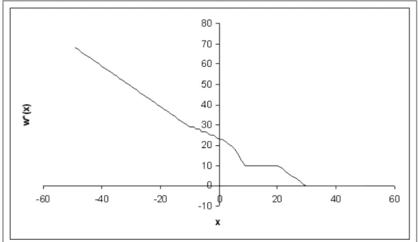
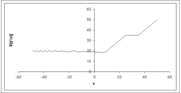
Uniform labor supply uncertainty: Uniform labor supply uncertainty models an ELSA with a large pool size. However the capability of the ELSA in finding skilled workers is variable. In this type of uncertainty if N workers are requested, acquiring each additional worker has a probability 1

N +1. Note that

the expected number of workers acquired increases as the number requested in-creases. On the other hand the probability of acquiring each additional worker decreases as 1

N gets smaller. Under this model the firm has equally likely chance

of acquiring 0 to N workers.

Normal labor supply uncertainty: We use normal distribution for an ELSA with a large pool size and a specific capability of finding workers with the required skill. If the firm requests N workers from the ELSA, the number of workers to be received is distributed with a normal distribution with mean µ ≤ N and a standard deviation σ. As the number of workers requested (N) increases, expected number of workers received and the standard deviation increases lin-early.

Binomial supply uncertainty with a decreasing probability of finding a worker: In this case the ELSA has a limited pool size and multiple customers with consistent demand rates. As the number requested from the ELSA increases, the probability of finding each worker decreases linearly. If the firm requests N workers, the number of workers acquired with a binomial distribution with rate of success equal to K−N

K , where K is the size of the ELSA’s worker pool.

Binomial supply uncertainty with an increasing probability of find-ing a worker: Under this settfind-ing we model an ELSA, preferrfind-ing larger sized demands. The ELSA avoids the division of its workforce by providing low avail-ability rates for small number of workers requested. As the number requested