Lot streaming in multi stage shops

I I3¥ #-f îi

Ä Ш іѣ іѣ

;?í3;;áég!UTt=í ΐ·5 Tí-. ТУг 'Гі; à іІрТріШ^^ ñ-í ·:ϊ= г ■, w* ад i!,» г3t· 2 J 3 iuiJut‘-_ ¿í¿ . rlM-.íM?‘.iA^'iT¡ú ϋ т!и/« ч>·· w г

i ' î ® i i r i ê i f £ e t i # i ; :. . . . ! Í 2 t Ч і i i - . , . i i I t U i r W u u . sí.a¡3· T i f £ , i i ' S I i l ' j ' r i - ’ · . Г · · Я 'V··í^ τ ’ , ·*Ι w r i * ϊ № · , i;% , . . w 2 . i . : t ' Г t s ' . ; L i t i s S l î l l c î : . .M В Щ 'zt ■· y >■ -;·-. Г.; " i»· ’a;? ... f . r k 3 a : ■ i t · · i ; ’■-:'! ·* i■■ v - î ù ;;í Έ ; t . | ‘¡-•■i.îuï'J .* ■ ' J r ü l 'i ' . f t . " ÏW S 'J . * ,í í: ï d ^ S Ü ѵ т : а ^ . JJr “. '“ i"· ' ' t 5 j* *“■·:·■ Í... Ll.J Z^. . . a^ ¡4'-' л; Îi?ja;;»S»· ,.:··ι. S« .j ¡s * Ü-.'.Î ¡/’лГіІ 1 tí .ftt 'í? ·;γ|* 4*í ^-■:«] -i ·:*-»?· t«“ 4î:t3 ■ ai :β a .; .?. v

,.ί ..U ■- a_i! aas -j -î· 5 ■ ίΡ ·? · · V - 4 ii ЩЦ> ■ « V &ÿ V.' ; 'te»· lï.VV \iUP<«'J·* (mrf ; Í 'W '

LOT STREAMING IN MULTI STAGE SHOPS

A THESIS

SUBMITTED TO THE DEPARTMENT OF INDUSTRIAL ENGINEERING

AND THE INSTITUTE OF ENGINEERING AND SCIENCES OF BILKENT UNIVERSITY

IN PARTIAL FULFILLMENT OF THE REQUIREMENTS FOR THE DEGREE OF

MASTER OF SCIENCE

By

Alper Şen

December, 1994

-А Ь7,У . S ' 4 İ - 1 Щ

I certify that I have read this thesis and that in my opinion it is fully adequate, in scope and in quality, as a thesis for the degree of Master of Science.

Assoc. Prof. Omer S. Benli (Advisor)

I certify that I have read this thesis and that in my opinion it is fully adequate, in scope and in quality, as a thesis for the degree of Master of Science.

Prof. ^г. Akif Eyler

I certify that I have read this thesis and that in my opinion it is fully adequate, in scope and in quality, as a thesis for the deaiete of Master of Science.

aAZ__^

__

^™f. Mustafa Akgul

I certify that I have read this thesis and that in my opinion it is fully adequate, in scope and in quality, as a thesis for the degree of Master of Science.

Assist. Prof. Selim Aktürk I certify that I have read this thesis and th at i

in scope and in quality, as a thesis for^tjier^i^f

ion it is fully adequate, ster of Science.

. Cemal Akvel

Approved for the Institute of Engineering and Sciences;

Prof. M ehm et^aray

ABSTRACT

LOT STREAMING IN MULTI STAGE SHOPS

Alper Şen

M.S. in Industrial Engineering

Supervisor: Assoc. Prof, Ömer S. Benli

December, 1994

In this thesis, a number of lot streaming problems in flow, open and job shops are investigated. Lot streaming is the process of splitting a job to al­ low for overlapping of its operations on various machines resulting in shorter completion times. When there is a single job, the problem is to find the size of the transfer batches (“subJots”) which minimizes a given performance mea­ sure (e.g., makespan, mean flow time). Multi-job problems are harder, since sequencing and sizing decisions must be made simultaneously. Most of the cur­ rent research in lot streaming is concerned with minimum makespan problems in flow shops. In this study, other performance measures and shop structures are also analyzed. Optimal sublot sizes are derived for the single job two ma­ chine flow shop mean flow time problem. Solution methods are proposed for the minimum makespan problem in open shops both for multiple job and single job cases.

Key words: Scheduling, Lot Streaming, Flow Shops, Open Shops, Job Shops

ÖZET

ÇOK MAKİNALI ATELYELERDE KAFİLE AKTARMA

Alper Şen

Endüstri Mühendisliği Bölümü Yüksek Lisans

Tez Yöneticisi: Doç. Dr. Ömer S. Benli

Aralık, 1994

Bu çalışmada çok makinalı atölyelerde kafile aktarma problemleri ince­ lenmiştir . Kafile aktarma bir işin bölünerek değişik makinalarda işlemlerinin çakıştırılması yoluyla akış zamanlarının azaltılmasıdır. Sadece bir tek iş oldu­ ğunda, problem, verilen performans ölçütünü enazlayan transfer kafilelerinin büyüklüklerinin bulunmasıdır. Sıralama ve büyüklük kararlan eşgüdümlü alın­ ması gerektiğinden, çok işli problemlerin çözümü daha güçtür. Bu konuda yapılan araştırmaların çoğunluğu akış tipi atölyelerde çizelge uzunluğu prob­ lemlerini incelemektedir. Bu çalışmada ise, değişik performans ölçütleri ve atelye tipleri İncelenmektedir. Tek işli, akış tipi, iki makinalı atölyelerde orta­ lama akış süresini enazlayan transfer kafilesi büyüklükleri hesaplanmaktadır. Çok işli ve çok makinalı atölyelerde çizelge uzunluğu problemleri için çözüm yöntemleri önerilmiştir.

Anahtar sözcükler: Çizelgeleme, Kafile Aktarma, Atelye Tipi Üretim

ACKNOWLEDGEMENT

I am very grateful to my supervisor, Associate Professor Ömer S. Benli for his invaluable guidance and motivating support during this study. His instruc­ tion will be the closest and most important reference in my future research.

I would like to thank to Assistant Professor Cemal Akyel for his efforts, guidance and encouragement in this research.

I am indebted to Professor M. Akif Eyler, Associate Professor Mustafa Akgiil and Assistant Professor M. Selim Aktürk for their keen interest in the subject m atter and valuable comments.

I would also like to thank to my classmates A. Aydın Selçuk and Abdullah Daşçı for their enlightening discussions.

Special thanks are due to Engin Topaloğlu, for his extensive cooperation. Finally, I would like to thank to my family and everybody who has in some way contributed to this study by lending moral support.

C ontents

1 Introduction 1

1.1 Problem D e fin itio n ... 4

2 Single Job M odels 7 2.1 Flow Shop Models 7 2.1.1 F o rm u la tio n s... 7

2.1.2 Two-Machine P r o b le m ... 11

2.1.3 Three or More M ach in es... .30

2.2 Open Shop M o d e ls ... 33

2.2.1 Single Routing M odel... 35

2.2.2 Multiple Routing M o d e l ... 38

2.3 Job Shop M o d e ls ... 38

3 M ultiple Job M odels 40 3.1 Flow Shop Models 41 3.1.1 Non-Preemptive M o d e ls ... 41

CONTENTS VIll

3.1.2 Preemptive M o d e ls... 43 3.2 Open Shop M o d e ls ... 43 3.2.1 Non-preemptive Single Routing M o d e l ... 45

3.2.2 Preemptive Multiple Routing Model 48

3.3 Job Shop M o d e ls ... 49

List o f Figures

1.1 Reducing flow times through lot stre a m in g ... 2

2.1 Sublot completion, Case 1: L = ( L i,. . . , Z-^+i,. . . , . . . . 17 2.2 Sublot completion, Case 1: L = ( L i,. . . , ¿„ + e, Lv+i — e ,. . . , Lg) 17 2.3 Sublot completion. Case 2: L — { L i,... ,L v ,L y ^ i,. . . , Lg) . . . . 18 2.4 Sublot completion. Case 2: L = ( L i,. . . , Z-t, + e, Z^+i ~ ■ ■ ■, Lg) 18 2.5 Sublot completion, TrLk > Lk+i, k = I , ... ,s 19

2.6 Sublot completion, optimal sublots 20

2.7 Sublot completion, non-optimality of consistent s u b lo ts ...25 2.8 Sublot completion, equal su b lo ts... 26 2.9 Sublot completion, lower bound on consistent sublot sizes . 27

2.10 Item completion, equal sublot sizes 29

2.11 Item completion, optimal sublot s iz e s ... 29 2.12 Network representation of a lot streaming problem ... 31 2.13 Gantt charts for machines and j o b s ... 35

LIST OF FIGURES

3.1 Time lags for lot streaming

3.2 Two-machine open shop, constructing the optimal schedule

. 42 . 46

List o f Tables

2.1 Two-Machine Mean Flow Time Problems 30

Chapter 1

Introduction

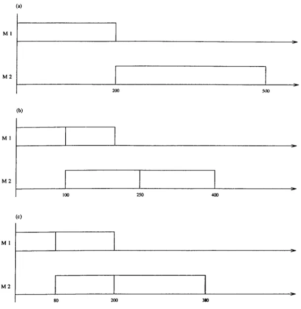
In classical scheduling theory, the job’s integrity is preserved while it is pro­ cessed and transferred. However, especially in batch manufacturing, it is prac­ tical to move some portion of the job to the downstream machine, before it is entirely completed on the current machine. Lot streaming is the creation of these transfer lots for a job, so that its operations can be overlapped on various machines. Lot streaming is applied by means of suhlots, which are the groups of items that are transferred from one machine to the next at once. Overlapping operations give the opportunity to start processing earlier on the downstream machines to achieve shorter completion times.

Consider the example, in which we have only two machines and a single job that consists of 100 identical units. Each unit requires processing of 2 minutes on the first machine and 3 minutes on the second machine. If lot streaming is not allowed, the job can be completed in 500 minutes (Figure 1.1.a). But, by simply transferring 50 units (half of the job) to the second machine, after they are complete on the first machine, it is possible to complete all the units in 400 minutes. We can also deliver these 50 units as soon as they are processed on machine 2. Hence 50 units will be delivered at time 250 and the remaining 50 will be delivered at time 400, resulting in an average completion time of 325 minutes (Figure l.l.b ), as compared to 500 minutes in the no lot streaming case. We are further able to reduce completion time to 380 minutes and average

CHAPTER 1. INTRODUCTION

completion time to 308 minutes, using sublot sizes 40 and 60 (Figure l.l.c).

(a ) M I ---200 500 M 2 (b) M 1 M 2 100 250 400 (c ) M 1 M 2 80 200 380

Figure 1.1: Reducing flow times through lot streaming

The use of sublots to accelerate operations is an important aspect in OPT systems. Umble & Srikanth [32], Lundrigan [17] and Browne et. al. [6] discuss that one of the key elements in OPT systems is the distinction between the process and transfer batches. “The transfer batch may not, and many times should not, be equal to the process batch”. Fogarty et. al. [11] state the importance of transfer batches in the context of drum-buffer-rope scheduling.

CHAPTER 1. INTRODUCTION

Jobs should be streamed on the non-bottleneck machines to enable the bottle­ neck machines to start their work as early as possible. The transfer of items is easily maintained by the use of resources (workers, material handling equip­ ment) at non-bottlenecks. Fogarty et. al. [11] also discuss that reducing sublot sizes (thus, increasing number of transfers) may be more efficient, than forcing process batch sizes to equal one as in JIT systems. Swann [25] and Vollmann [35] argue that conventional MRP techniques are no longer applicable, if over­ lapping operations are allowed. If parts are expedited by use of sublots, there is a need for designing (or revising) scheduling algorithms to get the possible benefits of OPT philosophy in an MRP system.

Overlapping of operations in scheduling is first considered by Mitten [18]. He proposed an algorithm to sequence multi jobs in a two-stage flow shop, in which each job may start processing on the second machine, a certain amount of time after it has started processing on the first machine.

Szendrovits [26] allowed for equal sized transfers between the stages and proposed a model to minimize the sum of setup, finished products inventory and work-in-process inventory costs, while meeting the continuous demand. The Economic Production Quantity of identical items that he optimized is processed uninterrupted on all machines. Truscott [31] studied the case where the sublot sizes can be multiples of a certain number and developed a model to minimize makespan in the presence of setup times, equal sized transfers and transfer times, again with the restriction that the machines should work continuously.

Baker [1] and Trietsch [29] relaxed the assumption that the sublots should be equal sized and proposed solution procedures to find the sublot sizes which minimize the makespan of a single job, with exogenously assigned maximum number of sublots. Since then, there is a considerable interest in lot streaming problems, of which the related portions are reviewed in the succeeding chapters.

The following section defines the lot streaming problem along with various models and restrictions.

CHAPTER 1. INTRODUCTION

1.1

P ro b lem D efin itio n

A resource that performs at most one activity at a time is called a machine. A shop is a collection of machines. An m-machine shop consists of m machines, Ml, M2, . . . , Mm- The activities are called jobs. There are n jobs, Ji, J2, · · ·, </n· Each Jj has m operations Oij. 02j, · · ·, 0,nj. Oij has a processing of duration Pij to be performed on A/, . No two operations can be processed simultaneously on a machine. A routing R = (M[ij, M[2],. . . , A/[„,]) for a job is the order of machines that will process the job. If this order is fixed for all jobs, the shop is called a Row shop. In an open shop, there are no such restrictions. In Job shops, each job may require more than m operations (hence each job may require same machine at different stages of its processing). Each job has distinct but a fixed routing in job shops. .\ job Jj consists of ty identical units. Hence, each operation is composed of Uj identical sub-operations, each of length Pij ~ P ijl^ j·

For a job, the group of units that are transferred at the same time from one machine to the next machine in the routing, forms a sublot of that job. For each Mi and for each Jj, there can be at most s,j sublots. We assume that the number of sublots is fixed in the shop for each job, i.e. = S j , i ■= \ , ... ,m .

In one extreme, Sj = Uj for each J, which implies a continuous flow production line, if the shop is a flow shop. In the other extreme, Sj = 1 for each j , which implies a classical scheduling model where each job’s integrity is preserved while it is transferred. The processing time of the kth. sublot for Jj on M, is pijLijk, where Lijk denotes the number of units in sublot. Clearly, Lijk = Uj for each Jj on each M,·. Cijk is the completion time of the kth sublot of Jj on A/,·. A job is completed, if all of its sublots are completed on all machines, that is, the completion time of Jj, Cj = max,-,;t Cijk.

If the number of units that form a sublot remains the same throughout the shop, then the sublots are called consistent, i.e. Lijk = Ljk for each Mi. Otherwise, they are called variable sublots. The size of the sublots may be restricted to take integer values, i.e. discrete case or the job can be assumed to be infinitely divisible, i.e. continuous case.

If each Jj is processed Pij consecutive time units on M,, over the time the machine is busy, then the shop is called a non-preemptive shop. If jobs can be processed with interruptions to allow for processing of units of a some other job, then the shop is called a preemptive shop. The shop is still a non-preemptive shop if the processing of a job is interrupted, but the machine is idle during the interruption. In any of these models, we do not allow for interruption of sublots on any machine. If a machine is not allowed to have idle time from the start of its first operation to the completion of its last operation, we say that the model is a continuous work model. Otherwise, we say that intermittent idling is allowed.

There may be several objectives, depending on the completion times of individual units (items), sublots or jobs. The job completion time may be critical for a system, in which each job is delivered as a whole. Items in a sublot may be assumed to be completed, when the sublot to which they belong is completed, resulting in a sublot completion time model. In item completion tim e models, each item is completed as soon as its operations are completed on last machine.

CHAPTER 1. INTRODUCTION 5

Under these models, the objective is a regular measure of performance, i.e. a monotone non-decreasing function of completion times. This may be the makespan, i.e. the time at which all the jobs (with all of their sublots and units) are completed. Стах — rnaxj Cj. Total flow time can be another objective, where we want to minimize the sum of job completion times, Cj. When the sublot completions are of concern, it is reasonable to weigh the completion time of each sublot with the number of units in it. That is, mean completion time of a job is, C[m]jkL[m]jk^ where [m] is the last machine in the routing of Jj. The objective can be easily revised for item completion time model. Similarly, all other relevant objectives, as well as the other elements of the theory of clcissical scheduling can be adapted to the lot streaming models.

The problem is to find the sizes (and routings if the shop is an open shop) of the sublots, and their sequence on machines so as to minimize the given objective function, subject to the restrictions mentioned above.

The purpose of this study is to propose solution methods for some of the untouched lot streaming problems. Chapter 2 presents the characteristics of the single job problem along with an extensive review of literature. The main contribution of this chapter is the Section 2.1.2 where we solve the two-machine mean flow time problem under sublot completion time model. The problem of routing and streaming a single job in an open shop is studied in Section 2.2. In Chapter 3, the multi-job lot streaming models are reviewed and studied. Section 3.2 and Section 3.3 present the first studies on streaming multi jobs in open shops and job shops. While different models in the literature are also reviewed, our derivations depend on the following assumptions.

• All units in a job are available at time 0. • Processing times are known.

• Jobs have zero setups.

• Material handling equipment is not a constraint neither in availability nor in capacity, except that the maximum number of sublots is limited. • Transfer times are zero.

• Jobs are infinitely divisible, i.e., sublot sizes may not be integer.

CHAPTER 1. INTRODUCTION 6

Chapter 4 discusses the main results of the thesis and directions for further research.

C hapter 2

Single Job M odels

Although their application areas may be limited, single job lot streaming mod­ els can be useful in understanding the nature of multi-job problems. They can also be utilized as a subproblem in exact or heuristic procedures to solve the multi-job problems. The research in single job problem concentrates in and is initiated by the flow shop problems with consistent sublots to minimize makespan. In this chapter, since single job models are analyzed, subscript j is omitted in variable definitions.

2.1

F low Shop M odels

2.1.1 F orm ulations

The basic lot streaming problem was first introduced by Baker [1]. In this problem, the sublot sizes are assumed to be consistent, i.e. Lik = Lk for each machine A/,·, so that the integrity of the sublot is preserved throughout the shop. The objective selected is the minimization of makespan. It is a convenient measure to observe the flow time reductions through lot streaming.

CHAPTER 2. SINGLE JOB MODELS

of the sublot k cannot start on M,, before the sublot (^ — 1) is completed on M,. The start of this sublot is also restricted by its completion in the previ­ ous machine, M,_i. With these constraints, the linear program to minimize makespan can be stated as.

min Cms subject to Cik > -k p. Z,/:, f = 1 ,..., m, = 1,.. Oik > -f-p.Tjt, ¿ = l , . . . , m , ¿ i » = k=l Cik > 0, k = l , . . . , s , f = Lk ^ b, k 1 , . . . , s , C^k b, k — C,o = 0, z = 1 ,... ,m. (2.1) (2.2) (2.3) (2.4) (2.5) (2.6) (2.7) (2.8)

Rather than minimizing makespan, the average time a unit spends in the shop can also be a measure of performance. The basic assumption that all the units in the job are completed, only when the whole job is completed may be a restrictive assumption. Customer service may be improved if we do not wait until the whole job is processed [21]. Assuming that each sublot is delivered as soon as its processing is completed in the shop (“sublot completion time model”), we have the objective of minimizing sum of sublot completion times, where each sublot is weighed by its size. The resulting model is a quadratic program with the objective function

LkCmk k=l

(2.9) subject to constraints (2.2)-(2.8). This quadratic objective function is first proposed by Kropp and Smunt [16].

Items can also be delivered, as soon as their processing is complete on the last machine (“item completion time model”). Suppose that there are s sublots transferred from Mm-i to Mm- Assume as if the last machine Mm processes s sublots. If Cmk is tlic completion time of the processing of sublot k on the

CHAPTER 2. SINGLE JOB MODELS

last machine, C„ik - PmLk will be the starting time of sublot k on Af„j. Since we assume that the number of units in a sublot can be fractional, the mean completion time of a unit in sublot k will be, {Cmk + Cmk — PmLk)/2. Hence, the consistent sublots formulation to minimize the mean flow time under item completion time will be.

s 1

min LkCmk - T^Llpr, k=l

subject to constraints (2.2)-(2.8).

(2.1 0)

An extension of this model, under the consistency assumption, can be used to minimize the number of tardy units. Suppose there is a due date, d, for the job, and the problem is to complete as many units as possible by this due date. A unit is tardy, if the sublot to which it belongs is tardy. If the optimal makespan, is less than or equal to d, then we are done, there are no tardy units. Otherwise, i.e., if > d, then append the constraint

C m , , s —\ — d (2. 11)

and optimize the objective function, m inL,,

subject to the Constraints (2.2)- (2.8), and (2.11).

When we allow for variable sublot sizes, simple lot streaming models are no longer applicable. The assumption that the number of sublots remains the same through the shop may be unrealistic in many production systems. These considerations lead to a systematically different model proposed by Benli [5]. This model is a periodic review model with variable period lengths, which are decision variables. The total number of transfers is h. = where s, is the number of transfers allowed from machine A/, to machine A/.+i. The periods are denoted by [T^, Tt+i], where Ti, T2, . . . , 7), are the times at which transfers

CHAPTER 2. SINGLE JOB MODELS 10

may take place. Define, A',..

L:,t

0,,i

Number of units produced on machine i in [Ti-i.Ti], Number of units transferred to machine z + 1 at time Tj, Number of units in the input buffer of machine i at time Tj, Number of units in the output buffer of machine i at time Ti,

1 if Li^t > 0, 0 if Li^t = 0.

Note that on any machine M,·, production can take place only in periods i , . .. ,h — rn + i, since the at least the first z — 1 and last m — z — 1 periods will be used for the transfer of products from machines Mi, A/j, · · ·, M,_i and M,+i, M ,+ i,... M„j, respectively. Then, we have the following mixed integer linear program to minimize makespan.

min Th

(

.

)

Ii,ti ^i,ti At,t ^ 0, Z 1, . . . , 771, t Z, . . . , /z 77Z T z, (2.19) Yi.t € {0,1}, z = 1 ,... ,m , t = z,. . . , /z - 77Z + z, (2.20)

where /¿^i—i — i — Oi,h—m+i — 0, i/o,o — Ljji,h — U and /z is a very large number or the capacity of the material handling equipment. The Constraints (2.13) and (2.14) are the inventory balance equations for the input and output buffers. Machine capacity constraints are (2.15). Constraints

CHAPTER 2. SINGLE JOB MODELS 11

(2.16) indicate whether a transfer takes place from a machine A/,· at time 7). Constraints (2.17) limit the number of transfers (sublots) at each stage. The formulation is adaptable to other problems like mean flow time minimization. Basic results of the lot streaming problem can also be obtained through the restriction of the general model.

2.1.2

T w o -M a ch in e P ro b lem

M inim izing M akespan

When the sublot sizes are consistent, we have the following linear program to solve the minimum makespan problem,

minC2s (2.21) Cik > Ci,k-l “1“p { i 1)2, L· (2.22) C2k > Cik + P2-^/:? ^ 1) · · · ) *5, (2.23) ± L , = (2.24) k=l Cik > 0, i = 1,2, Â: = 1 , . . . , 5, (2.25) Lk > 0, k =: 1 ,...,5 , (2.26) Cio = 0, i = 1,2, (2.27)

This problem was studied by Baker [1] and Potts & Baker [20]. Baker [1] used the LP formulation to derive the solution. Potts Sc Baker [20] showed that the makespan is equal to the sum of

• The processing time of sublots I , . .. ,k on M i, and • The processing time of sublots k , . . . , s on M2

for any sublot k and hence each sublot is critical'. The solution is given by the “geometric” sublot sizes, i.e.,

1 — 7T

Li - U

CHAPTER 2. SINGLE JOB MODELS 12

Lk = TfLk-i, k = 2---- ,5, (2.29)

where tt =

p^lpi-The discrete version of the problem is studied by Trietsch [29]. He proposed an iterative algorithm of time complexity ^ ( s ) to find the optimal integer sublot sizes. Trietsch L· Baker [30] analyzed the cases, where the transportation times in between machines are not negligible and the transporters have limited capacity.

VARIABLE SUBLOTS

If we allow for variability in the sublot sizes in each stage, one would expect that any regular measure of performance would improve. This is simply based on the fact that, for these measures of performance, consistent sublots are subsets of variable sublots. The question is the following: when is it sufficient to consider only the consistent sublots in the search of optimal (variable) sublots? When the objective is the minimization of makespan, Trietsch & Baker [30] state that it is not necessary to consider the variable sublot sizes since there is is only one set of transfers. Note that, here the transfer of items from second machine is not considered.

EQUAL SUBLOTS

The optimal solutions for the two-machine flow shop problems result in dif­ ferent sublot sizes. However, it may be more practical to use equal sublot sizes. In this section, we will compare makespan obtained by using equal sublot sizes, F ^{L ), with the optimal makespan, F*{L), using the ratio, F ^{L )/F '‘{L). For notational convenience, we shall assume that U = 1, = 1 and p2 = tt.

When equal sublots are used, makespan is.

F^{L) = rnax{l/s -f- tt. 1 -f tt/s}. On the other hand, optimal makespan is.

CHAPTER 2. SINGLE JOB MODELS 13

Potts & Baker [20] have shown that,

F ^ { L )/F ^ L ) < 1.09.

M in im izin g M ean Flow T im e u n d e r S u b lo t C o m p letio n T im e M odel

Suppose, an item leaves the shop when the sublot to which it belongs is com­ pleted in the last stage. In a 2—machine flow shop, the flow time of all units in the job will sum up to L2kC2k- This is equivalent to mean flow time, which is the average time a unit spends in the shop, h Ej=i L2kC2k- Thus the problem, with consistent sublots, becomes a quadratic programming problem with the objective function

S

E ^^kC2k, (2.30)

k = l

subject to Constraints (2.22)-(2.27).

An efficient solution procedure, proposed for the two-stage flow shop prob­ lem with consistent sublots is given below. In this problem one has to consider two cases: (f) tt < 1, and (n) tt > 1, where tt = P2İP1· Çetinkaya & Gupta [8], independently, obtained the same result for the first case, and they conjectured but not proved the result for the second case.

CASE I : 7T < 1

As discussed in Şen et. al., [27], consider the general case. There are in machines, with the property pi > max2<,<m{Pt}, and we will show that equal sublot sizes (i.e. Lk = U/s A: = 1 ,... ,s) are optimal.

We first need the following result showing that there exists an optimal solution with nondecreasing sublot sizes.

R e su lt 1 If Pi > max2<Km{Pi} then an optimal solution exists where;

CHAPTER 2. SINGLE JOB MODELS 14

To prove this result, Şen et. al. [27] showed that any schedule that does not satisfy (2.31) can be converted to a schedule which satisfies (2.31) without increasing the mean flow time. Suppose we are given the sublot sizes L = { L i,... 1 Ls) which are claimed to be optimal and for at least one k , Lk > Lk+i- An iterative procedure is designed for achieving a schedule which satisfies (2.31). At each iteration v, maximum sized sublot among the first s — v sublots is replaced at the {s — v) th position in the schedule. In s iterations, the resulting schedule satisfies (2.31). It is also shown that at each iteration, the mean flow time does not increase.

Çetinkaya & Gupta [8] proved the same result using the following Lemma by Miyazaki k Nishiyama [19],

L em m a 1 For the ordinary flow shop problem (without lot streaming) to min­ imize weighted flow time (Y^wjCj), job h precedes job I in the optimal schedule if,

i) 10k < We

ii) Wh ZT=i Pr,h < we ET=i Pr,t, i = 1 ,..., m where, wj is the weight of job j .

Consider our problem as a weighted flow time problem, with sublots con­ sidered as jobs. The processing time of job k on machine i is piLk and weight of job k, lük = Lk- Note that,

m m

Lk ^ Le ^ Lk^(^Pr Lk ^ Le ] p^Le·

r = i r = i

It is easy to see that sublot k precedes sublot H if Lk < Le- Then, the result follows.

With this property, the following formulation with a convex function and fewer constraints can be obtained. Assuming U = I,

minY)^ LkCmk k=l

CHAPTER 2. SINGLE JOB MODELS ₁₅ v=2 subject to C,nk = P iY ^ L c P LkY^p^,. k = l , . . . , s ,

^=l

R e su lt 2 An opti7nal solution to the above problem is

Lk = - .

s k =

P ro o f: Let the Lagrangian function be,

5 A:—1 m s

£ ( L i , Ls,6) = J2 M pi + Lk E py) + Lk - 1),

i t = l t - l v-\ k = \

then dC

dLk = P iY ^ L tP 2Lk Y^py - piLk + S = 0, andu = l

BC

®

Since,

Lk = { - S - p i ' ^ L i ) l { 2 ^ p y - p i ) , A: = l , . . . , s

^=1

Y^k-i Lk = ^ implies that j is the candidate optimal solution. However, to prove that it is the desired solution, we have to show that the objective function is convex. The Hessian matrix of the objective function is,

a b b b b .. b a b b b .. b b a b b .. 11= b b b a b .. b b b b a ..

CHAPTER 2. SINGLE JOB MODELS ₁₆

where a — pi^ and b = pi.

In order for the objective function to be convex, the Hessian matrix should be positive definite. In a positive definite matrix, every upper left sub-matrix should have positive determinant. Let H i , . , Hr, ...,H s = H be the upper left sub-matrices of H. The determinant of Hr can be found to be,

d e t ^ , = 6 ^ ( ^ - i r - ' ( ^ - F r - l ) (2..32) since a > b. It is clear that, det Hr > 0, r = 1 , . . . , s.

CASE II : 7T > 1

Again assume, without loss of generality, that 17 = 1 and the processing time of the job is 1 on the first machine and tt{ = pa/Pi) on the second machine.

Since p2 > Pi ■, we have tt > 1.

R e su lt 3 When tt > 1, wLk > Lk+i, k — I , . . . s — I, in an optimal schedule.

P ro o f : Suppose the contrary, i.e., there exists an optimal solution L = { L i,. . . , Ls) such that, at least for one k, wLk < Lk+i- Let v — mini<jt<s_i{^ | irLk < Lk+i}. A new solution can be constructed for some e > 0, as

Lk = Lk, k = l , . . . , v - i Ly — Ly -j- e,

Lu-f-i —

Lk = Lk, k = u -b 2 , . . . , s.

It is sufficient to show that the new solution, L is feasible and F{L) < F{L). Since E]b=i Lk = Eyt=} Lk, and Ci,y+i = Ci.,.+i = E t t l Lk, for feasibility, it is enough to show

C'2,t;+l £ C2,v+l- (2.33)

We will now show that (2.33) holds and F( L) < F{L) for the following two possible cases.

CHAPTER 2. SINGLE JOB MODELS 17

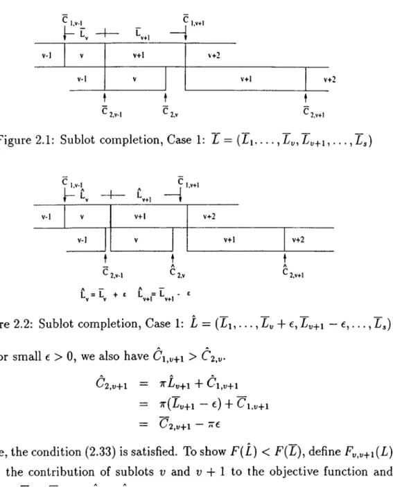
C ase 1 : > C'2,u (See Figure 2.1 and Figure 2.2).

l · “

1

K+1

v-1 V v + l v+2

v-1 V v+1 v+2

- 2.V-I ' 2,v ' 2.V+1

Figure 2.1: Sublot completion, Case 1: Z = ( i i . . . . , Ly-|_i, . . . ,

l.V'l , l.VTl l · “ ‘ 'v --- K u — 1 v-1 V v+1 V + 2 v-1 V v+1 v+2 ' 2.V-1 '2.V ' 2.V+1 L = L _{V V}+ e L = L _{v+1 v+1}- £

Figure 2.2: Sublot completion, Case 1: L = ( L i , . . . , + e, — e, . . . , L^) For small e > 0, we also have Ci,u+i > C2,v

G2,v+1 = ^Lv+l + Ci^v+l

= ir(Lv+i — e) + Ci,v+i

= C 2 , t , + 1 — 7T£

Hence, the condition (2.33) is satisfied. To show F(L) < F{L), define

to be the contribution of sublots v and u + 1 to the objective function and Uv,v+i ^ Ly -\- Tv+1 — Ly Lv+i·

F y ^ y ^ l { L ) — + Z / u ( l + 7 r ) ] Z - „ + [ ( C ’ i , i ; - 1 + ¿ u + T v + i ) + 7 r T u + i ] Z / i , ^ . i

= ( i + 2 r ) T : + ( f / „ ,u+l + T^Ly+x )iv+l + Ci^y-iUy^v-x-i = (1 + '^)Ly + Uy^y+iLy^-i + X ¿u+1 + G\^y-iUv^y+i Similarly,

Fy^y^i{L) = (I + t)LI + Uy,y+iLy+i + + Ci^y-iUy^y+i

CHAPTER 2. SINGLE JOB MODELS 18

then,

Ev,v+i{L) — = —(27t + l)e^ + (2r + — 2L„)e = - ( 2 ; r + l ) e 2 + (27r + l ) ( I , + i - I „ ) e

But, we know that ttL^ < Lt,+i, thus L^ < Lv+i, therefore it is clear that Fv,v+i(L) - Fv ,v+i{L) is positive for some e > 0. Hence. F{L) > F{L), for some e > 0.

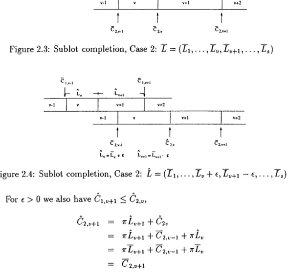
C ase 2 : Ci^v+i < C2,v (See Figure 2.3 and Figure 2.4).

C,.v. Ly —f— Ly^j v-I V v+1 v+2 v-1 V v+1 v+2

_1

_t

_1

Figure 2.3: Sublot completion. Case 2: L = ( Li , . . . , ¿„+1, . . . , L^)

c,.v ., c , i - L , - 1 - L „ , ,V+1 V-1 V v+1 v+2 v-1 V 1 v+1 v+2 c,.

Figure 2.4: Sublot completion. Case 2: L = ( Z i , . . . , + e, Ly^i — e , . . . , Zj)

h a v e C i ^ x j ^ i _{^ ^ 2 , V I t} C ' 2 , u- f l = 7 r Z „ + i + C 2 V — 7t Z v + i + ^ 2 , 1 — 1 - I - 7t Z „ — 7 T L v + i - f - C 2 , t -1 + 7 r Z „ z = C 2 , v + l

CHAPTER 2. SINGLE JOB MODELS 19

since + = L„ + Z„+i. Hence, (2.33) is satisfied. To show F(L) < F{L), Tv,v+l(L) — (C2,v-1 F'^Li.)Li, (C2,v-1 -l· '^Fv ,u+l)Ly^l -7-2 — 7T ~ J^v) + f-^v,v+l02,v-l Similarly, then, A A A _ _ _ _

Fi,^v+i(L) '^L^ T Ly) T Fy,v+\02,y—\

= T^{Ly + e)^ + T^Fy,y+i{Fy^y+i — Ly — t) F /7v,u+iC'2,i—i

Fy^y+i{L) - Fy^y+i{L) = -ire^ F {Fy,y+i - 2Ly)Trc

= —TTC^ + (Tv+1 - Ly)i:e.

Since (Ty+i — Ly)7T is positive, Fy^y+i{L) — Fy^y^i{L) is positive for some c > 0. Thus, F{L) > F{L) for some e > 0. Thus in any optimal schedule, 7TL k ^ Tfc+l A'=:1,...S — 1. □

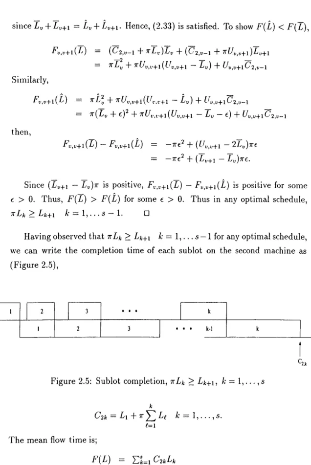
Having observed that nLk > Lk+\ Ar = 1, . . . s — 1 for any optimal schedule, we can write the completion time of each sublot on the second machine as (Figure 2.5),

1 2 3 • f · k

1 2 3 0 • · k - 1 k

Figure 2.5: Sublot completion, TrLk > Lk+\, A’ = 1, . . . , s

‘'2,k

C2k — ¿ 1 + 7T L( A — 1 , . . . , s.

e=i

The mean flow time is;

F{L) = Y:UiC2kLk

CHAPTER 2. SINGLE JOB MODELS ₂₀

Then, an equivalent reformulation of the problem is, 5 k ininF(L) = Li k=i e=i s subject to ' ^ L k = 1, Jt=l Lk+\-TrLk < 0, k = l , . . . , s - l , Lk ^ 0, A; = 1 , . . . , s. (2.34) (2.35) (2.36) (2.37)

R e su lt 4 The following sublot sizes are optimal for (2.3^)-(2.37),

Lk = TT^-'^Li, k = l , . . . , v , (2.39) Lk = --- ---, k = v + l , . . . , s (2.40) (s - u) ifirTv > Tv+1 > Lv and v < s. v-2 Y-1 V v+l v+2 v+3 Yfi v-3 v-2 v-l Y Y+l v+2 v+3

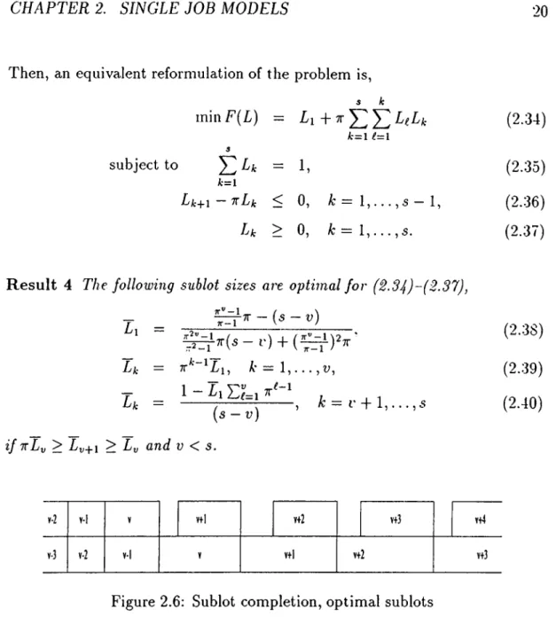
Figure 2.6: Sublot completion, optimal sublots

P ro o f : The Gantt chart for an instance of the above sublot sizes will be as shown in Figure 2.6. Since the objective function can be shown to be convex, it will be sufficient to show that the above solution is a Karush-Kuhn-Tucker point. The Hessian matrix for the objective function is,

2 1 1 1 1 . . 1 2 1 1 1 . . 1 1 2 1 1 . . H = 1 1 1 2 1 . .

CHAPTER 2. SINGLE JOB MODELS 21

The determinant of each upper left sub-matrix of H is positive since, from (2.32) we have,

det Hr = r + l, r =

Hence, the Hessian matrix is positive definite and the objective function is convex.

Assign, Lagrange Multipliers 6 for (2.35), and A^,- for (2.36). As seen in Figure 2.6, only the first u — 1 of the type (2.36) constraints are binding. So Karush-Kuhn-Tucker conditions for the solution are.

For Li

1 LI — ttAj — 0.

For Lk A: = 2 , . . . , u — 1

7T + irLf; + <5 + Afc_i — TrAfc — 0. For L, For Lk A: = u -f 1 . . . , 5 7T -f- wLy -H ^ + Au_x — 0. A "t" TrLjt ■}■ — 0. (2.41) (2.42) (2.43) (2.44)

We have the following solution to the system (2.41)-(2.44). Using the values L = ( T i ,. . . , Ls), and noting th at Lk = Ls k = u + 1,. . . , s, we get from (2.44),

^ “ 7 T 7 T L/^ y (2.45)

We also get from (2.43) and (2.45),

A^._i — 7t(Tj Ty), (2.46)

which is nonnegative. From (2.42) we obtain.

CliAFTER 2. SINGLE JOB MODELS ₂₂

Ajk = TrAjt+i + x{Lg — Lk+i) k = I , . .. ,v - 2 . which together with (2.46), proves the non-negativity of At k We have from (2.46) and (2.47),

A i = ( ^ — ^ ) I . - (

7T — i TT^ — 1 ) i .·

(2.47)

(2.48)

On the other hand, (2.41) and (2.45) give, 1 -f- ttLi — ttLs

Ai —

7T (2.49)

We also need to show that the sublot sizes result in a consistent solution of Lagrange multipliers. I + ttLi - ttL, ^ -TT — ~ --- 1 _7T — t ---_{7T — 1}7·/^« ~ 1. _{TT^ — 1 -)^1} Using (2.40), . 7 r ' ' - T — TT^” — 7T^ — — — 1 7T — 1 7T^ — i 7T 7T — 1 (s — u) 7T^ — 1 ^ X ,7r‘' - U 1 1 Lx 7Γ^'' -— l ^ ( s -— u) X ^ x — l ^ ( s — r ) ^ x^ — 1 which results in.

¿ 1 = □

f e ^ x ( s - u ) + ( ^ ) ^ x

For u = s (i.e. all the sublot sizes are geometric), we have the system of equations (2.41), (2.42) and (2.43). The system has a consistent solution, hence it is enough only to show the non-negativity of the Lagrange multipliers, Afc, ^ = 1 , . . . , s — 1. We have,

-x^* -f- 2x"+i + 2x* - 2x - 1 ■^s-l —

CHAPTER 2. SINGLE JOB MODELS ₂₃

5 — < — 1 5 - 1

Aji· = A,_1 ^ 7T^ + { L s - L()k^

<f=0 ^=/.-+1

Since Ajt > Aj_i k = 1 ,... 5 — 2. it is sufficient to check the non-negativity of As—1.

Hence, all the sublot sizes are geometric (u = s), only if the polynomial in the numerator of is positive for a given tt, since the denominator is always positive.

Combining these results, the following algorithm solves the problem: A lg o rith m I

u <— 0, optimal^—FALSE

If / (tt) = -Tr2^ -h 27T*+^ + 27T* - 27T - 1 > 0

optimal i— TRUE, geometric sublots are optimal

W h ile n o t optimal u <— u + 1 Ll [ ^ 7 T - (s - u)]/[$fp-7r(5 - u) + ( ^ ) ^ 7t] Lk <— k = 2, . . . ,v Lk ^ [ l ~ Li E L i - ^)]> k = v + l , . . . , s if 7T L y ^ L y ^ \ ^ L yy

optimal <— TRUE, T = ( L i,.., Tj) is optimal

For certain values of s, closed form solutions can be obtained. These solu­ tions can be obtained by determining the intervals of tt in which — Lyj^i and Lyjfi — Ly is positive for u < s and / (tt) is positive for s. Sample solutions for s = 2 and s = 3 are given below.

CHAPTER 2. SINGLE JOB MODELS ₂₄

S o lu tio n F or 5 = 2

, r . r . . i ( 4t. * ) + ^ ( ^ . 1 ? ) i t l + v / 2 < x

In the first interval of tt, the sublot sizes are geometric (v = $ = 2), while in the second u = 1. S o lu tio n For 5 = 3 1 2 + ’ TT^-fTT + l ’ 7t2 + /T|1 -/1 TT^ + TT-l l7i£j:£^_z£ 1 7r^-f27T+l V 2 TT^+TT^ + TT ’ 2 7T^-f-7t2-f 7T ’ 2 + ( TT-fl TT+l \ V 37T ’ 3 ;r ’ 3;r / if 1 < 7T < (1 + \/5)/2 i ) i f ( l + v / 5 ) / 2 < 7 r < ( 3 + v / T 3 ) / 2 if (3 + \/r3)/2 < 7T

In the first interval of tt, the sublot sizes are geometric (u = 5 = 3), in the second V = 2, and in the last interval u = 1.

VARIABLE SUBLOTS

Although the consistent sublots are optimal in the job completion case, they are not necessarily optimal for the sublot completion case. The following example shows that when the objective is the minimization of sum of sublot completion times, consistent sublots do not result in global optimality. Note th at in this case there is a second set of transfers from the second machine.

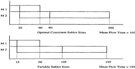
Consider the following example : 60 units \vill be processed on a two- stage flow shop and pi = 1 and p2 = 3. There are two sublots available. As shown in the sample solution above and since tt = 3 the optimal consistent sublot sizes are 20 and 40. These sublot sizes result in a mean flow time of

¿ (2 0 X 80 -h 40 X 200) = 160 (Figure 2.7).

But, we can achieve mean flow time of ¿(3 0 x 105 -f 30 x 195) = 150 by using sublot sizes (15, 45) on the first machine and (.30, 30) on the second machine (Figure 2.7) .

CHAPTER 2. SINGLE JOB MODELS 25 M I M 2 2 0 M I M 2 15 6 0 8 0 O p t im a l C o n s is t e n t S u b lo t S iz e s 2 0 0 M e a n F lo w T i m e = 160 6 0 105 V a r i a b l e S u b lo t S iz e s 195 M e a n F lo w T i m e = 150

Figure 2.7: Sublet completion, noii-optimality of consistent sublots the following conjectures, without proofs.

C o n je c tu re 1 Mean flow time is minimized by equal sublots on each stage if

P i >

P2-C o n je c tu re 2 Mean flow time is minimized by geometric sublots on first stage, and equal sublots on second stage if p\ < p2

-These conjectures depend on the continuous production on dominant machines. For Pi > P2i the first machine is dominant, and determines the sublot sizes. For Pi < P2i the dominant machine is the second one and geometric sublots on the first machine provide the minimum idle time for second machine which allows continuous production. Thus, operations on the second machine start as early as possible and since geometric sublots on the first machine provide required input, equal sublots are obvious on the second machine. Note that, the Conjecture 2 in addition gives the alternate optimal solution to the minimum makespan problem.

EQUAL SUBLOTS

The optimal sublot sizes are derived for the consistent case and conjectured for the variable Ccise in previous sections. Recall that, for tt < 1, equal sublots

CHAPTER 2. SINGLE JOB MODELS 26

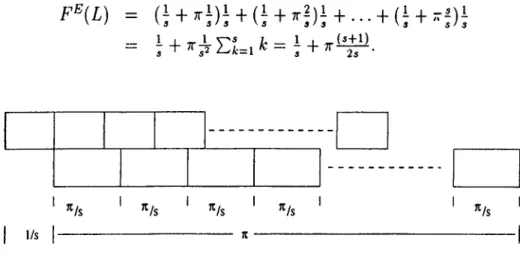
are optimal. For the case tt > 1, mean flow time with equal sublot sizes is (See Figure 2.8),

1/s

' ^1$ ^ ^Is ' ^1$ ---

)t---^/s

Figure 2.8: Sublot completion, equal sublots

Since it is not possible for general s to derive explicit expression for the optimal mean flow time that can be achieved by the consistent sublots, F^{L), we shall use a lower bound for its value. We know (from Result 3) that,

7TLk ^ Lf;^i, fc = l , . . . , s 1, is a necessary condition for optimality.

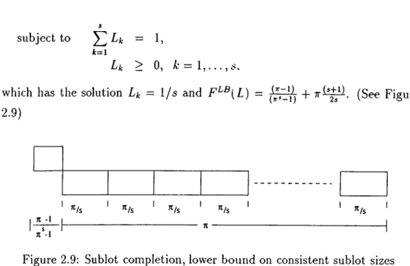
Consider the following linear program: ^ = min L\

subject to TrLjt > Ljt+i, A: = 1 , . . . , s — 1,

- 1,

k=l

Lk > 0, A: = 1 ,... ,5 — 1.

It is not difficult to show that 2 = Thus, the smallest possible size of the first sublot on Mi is 2. Since pi = 1, 2 is the earliest time M2 can start processing. Once M2 starts processing, it will continue uninterrupted because

7T > 1. Thus a lower bound for the optimal flow time, F ‘^{L), is given by the minimal value of the following quadratic program,

CHAPTER 2. SINGLE JOB MODELS ₂₇

subject to E i . = 1.

k = l

Lk ^ k = ^ s.

which has the solution Lk = l / s and F ^^ ( L ) = (See Figure 2.9) ^/s n -1 ^/s ' ^/s --- Ji---^/s n -I

Figure 2.9: Sublot completion, lower bound on consistent sublot sizes

We have F^^{L) < F^{L). Thus, F ^ { L ) / F ^ { L ) < F ^ { L ) / F ^ ^ { L ) where,

i _L Trif+ll F ^ { L ) / F ^ ^ { L ) = - " 2*

iiz ill 4 _ T r k h i l '

Result 5

1.14.

Suppose s can take any real value, then, /(Tr,^) = F ^ { L ) I F ^ ^ ( L ) is a continuous function of $ and tt for s > 2 and tt > 1. Then, we set the partial derivatives with respect to s and ~ equal to zero. These two non­ linear equations are solved numerically by Maple V ©, giving a single solution (7T*,s*) = (1.938,4.267). The solution (tt' .s*) gives /(;r*,s*) = 1.14. This single solution is a maximum point, since

= _0.00184.

OTTOS OTT^ os^

It is obvious that, for discrete values of s the function’s maximum is less then the one we have found. Consider the solution ( ^ ,5) = (1.992,4). These values result in the ratio 1.139, which is very close the ratio found using (7r“,s*).

The construction of the lower bound for the consistent sublot sizes gives the optimal variable sublot sizes that we have conjectured, that is geometric

CHAPTER 2. SINGLE JOB MODELS 28

sublots on the first machine, equal sublots on the second machine. Since F*{L) is the mean flow time achievable by variable sublots, we claim the above result holds for the variable sublots ( F ^ ( L ) /F ’ (L) < 1.14).

M in im izin g M ean Flow T im e u n d e r Ite m C o m p le tio n T im e M odel

In this case, an item is assumed to be completed as soon as it completes processing in the last machine. When continuous sublot sizes are allowed, this is equivalent to assuming infinite number of transfers in the last stage. In the case of two-machine flow shop with consistent sublot sizes, the objective function is

m \ n j2 [C2k - { P2/2)Lk] Lk

k = l

subject to Constraints (2.22)-(2.27).

Again we have two cases to consider: {i) tt < 1, and (ii) tt > 1, where 7T = P2/P1· L· Gupta [8] have shown that, if tt < 1, then equal size sublots are optimal, otherwise it is optimal to use the geometric sublot sizes as given in equations (2.28) and (2.29).

EQUAL SUBLOTS

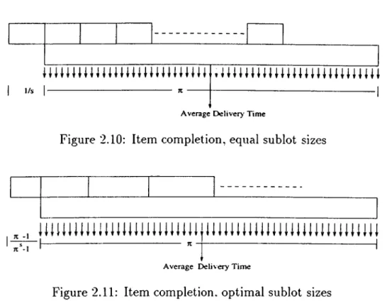
Note that, equal sublots are also optimal, when x < 1. Therefore, we again consider the case x > 1, in which geometric sublot sizes are optimal. Equal sublots give the following mean flow time (See Figure 2.10 and Figure 2.11)

F^iL) = l / s + ir/2,

since all the items can be assumed to be delivered at time I/5 + x/2. For the optimal sublot sizes we have a similar form:

(x - 1)

(x* - 1) + Tr/2·

CHAPTER 2. SINGLE JOB MODELS 29

1 >/» 1

. u m u m m u u u u m u i 1 1

Average Ctelivery Time

Figure 2.10: Item completion, equal sublot sizes

71 -1 7 l’‘- l

I t l l l l l U i l l l I t t i m i t l l l l j l l U t U l l l l l l l l U t l l l U l l l I U

”T

Average Delivery Tim e

Figure 2.11: Item completion, optimal sublot sizes

This result is obtained by a similar approach to the one used in Result 5. For s = A and tt = 2.021, the ratio turns out to be 1.172.

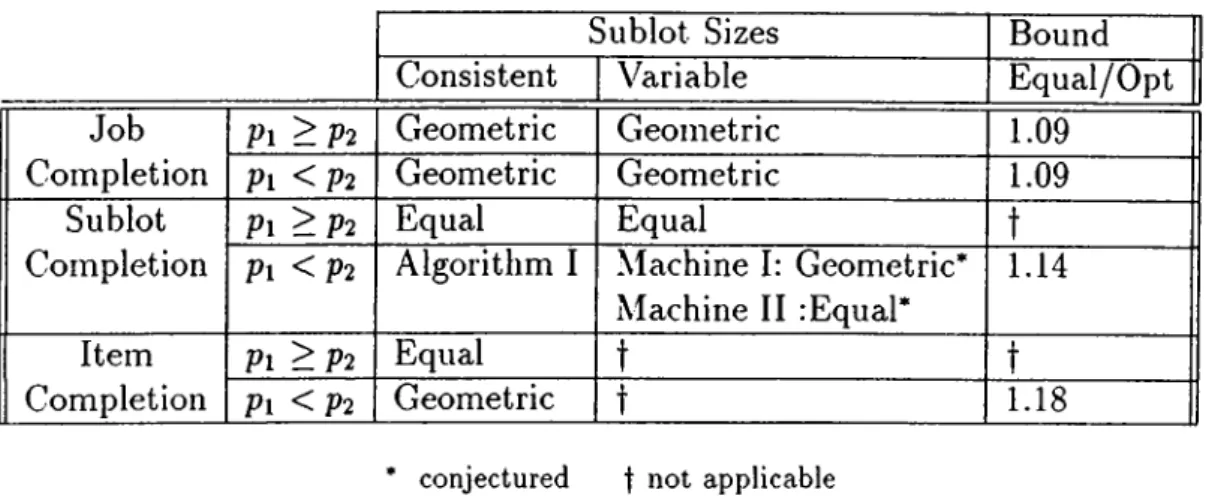
In this section we analyzed lot streaming of a single job in a two-stage flow shop. Makespan minimization problem can be viewed as a mean flow minimization problem under the job completion time model. Where applicable, consistent and variable sublots are separately treated. The implications of equal sublots, which are widely used in practice are also presented. Table 2.1 summarizes the results of minimization of mean flow time in a two-stage flow shop.

Except in Sublot Completion Time Model with pi < p2, consistent sublots are optimal in other cases even if variable sublot sizes are allowed. As seen from the last column, equal sublots are quite effective. Thus, the practical use of equal sublots may be justified.

There may be other streaming policies applicable to the two-machine flow shop. Some instances may allow infinite number of transfers (unit transfers) between machine 1 and machine 2. In this case, equal sized deliveries are

CHAPTER 2. SINGLE JOB MODELS 30

Table 2.1: Two-Machine Mean Flow Time Problems

Sublot Sizes Bound

Consistent Variable Equal/Opt

Job Completion Pi > P2 Geometric Geometric 1.09 Pi < P2 Geometric Geometric 1.09 Sublot Completion Pi > P2 Equal Equal t

Pi < P2 Algorithm I Machine I: Geometric* Machine II :Equal* 1.14 Item Completion Pi > P2 Equal _{t t} Pi < P2 Geometric t 1.18

* conjectured f not applicable

obvious. Some other models may allow different number of sublots at each stage. While specific instances should be studied for analytical results for this problem, the general model of Benli [5] presented in section 2.1.1 provides a mixed integer linear (or quadratic) programming formulation.

2 .1 .3

T h r e e or M ore M a ch in es

When there are three or more machines and the consistent sublots are used, linear programming and quadratic programming formulations are available for minimum makespan and minimum mean flow time problems.

Potts & Baker [20] observed that the flow shop problem with process­ ing times p i , . . . , p i , ... ,pm, and the inverse problem with processing times pm ,·· · ,pm-i+i,· ••,Pi are equivalent.

Baker [1] studied the three-machine problem with two sublots and obtained results similar to that of the two-machine problem. Glass et. al. [12] used the network representation of the lot streaming problem to provide solutions for the three machine problem with s sublots. A vertex (¿, k) is defined for each machine i and for each sublot k, with weight piL^· Directed edges from vertex (z, k) to vertex (z + 1, fc) for z = 1 , . . . , m — 1 and /¡: = 1 , . . . , s ensure that sublot

CHAPTER 2. SINGLE JOB MODELS 31

k can start processing on machine i + 1 only after it is completed on machine i. Directed edges from (¿, k) to (», + 1) for f = 1 , . . . , m and it = 1 , . . , , s — 1 ensure that machine i can start processing sublot k + l, only after it completes the processing of sublot k. The length of a path is defined as the total weight of vertices that are on it. The longest path from vertex (1,1) to vertex (m,s), referred to as critical path, gives the makespan. A 3-machine 4-sublot problem is depicted in Figure 2.12.

S u b lo i 1

M a c h in e 2

M a c h in e 3

Figure 2.12: Network representation of a lot streaming problem

Glass et. al. [12] showed that, in an optimal solution, all sublots are positive. This intuitive result states that all the possible transfers will be utilized to accelerate the production. Using network representation of the problem. Glass et. al. [12] derived the optimal consistent sublot sizes for the three-machine minimum makespan problem.

R e s u lt 7 In a three-stage flow shop, if p\ < pipz optimal sublot sizes are Li = i ~ ~ 1)’

1 1/^, if Pi = P 3 ,

Lk = k = 2, . . . , s ,

CHAPTER 2. SINGLE JOB MODELS 32

R e s u lt 8 In a three-stage flow shop, if p\ > pipz optimal sublot sizes are Lk = L„ = Lk = ^\Ly, h 1, l/[(9i ~ l)/(9i ~ 1) + - 1)/(9з - 1) - 1], if P\ -ф P2,p-2 ф Рз, 1/[г - 1 + “ l ) / ( ? 3 - 1)], if Pi = P2,P2

Ф

where v can be easily found by bisection search in { I ,...,« } and q\ = Pi/p2,

93 = P3/P2·

When the sublot sizes are not restricted to be consistent, the three-machine problem can be solved by a procedure proposed by Trietsch & Baker [30].

When interm ittent idling is not allowed, the two-machine solution can be applied independently to the consecutive machines to find the variable sublot sizes which minimize makespan.

When the objective is minimization of the mean flow times, note that the results presented in Section 2.1.2 for the case pi > p2 is applicable to m- machine problem for the case pi > max2<,<m{pi). Thus, equal sized sublots are optimal for minimizing mean flow time under sublot and item completion time models, when the processing time on the first machine is greater than processing times any of the other machines.

The two-sublot problem received a greater attention, since marginal returns diminishes as the number of sublots increases. Baker L· Jia [3] reported that two or three sublots are sufficient to obtain most of the benefit that can be achieved by lot streaming. Furthermore, two-sublot solutions can be used in developing heuristic methods in s-sublot problems.

Baker Sz Руке [4] and Williams & Tüfekçi [36] studied the two-sublot makespan minimization problem. They derived algorithms of complexity O(m^) to calculate the optimal sizes of the consistent sublots and used it in heuristics to compute the sizes of multiple sublots.

CHAPTER 2. SINGLE JOB MODELS 33

Topaloglu et. al. [28] and C^etinkaya & Gupta [8] proposed 0 { m ‘^) time algorithms to find sublot sizes that minimize mean flow time under sublot and item completion time models.

2.2

O pen Shop M o d els

In open shop problems, since one is able to choose any routing for the jobs, it is possible to obtain shorter makespan than the flow shop problems. How­ ever, this flexibility also adds complexity to both formulation and solution of open shop problems. Therefore, the current research is limited to minimum makespan problems. Before analyzing the lot streaming problem, the basic properties and results in open shops will be summarized.

An open shop schedule must satisfy the following two sets of constraints,

• No two jobs can be processed simultaneously on a machine. T hat is, for each Mi and for each pair of jobs (Jj, Jyt),

either Cij > Pij -f Cik or ^ Pik T Oij. (2.50) • No two machines can process a job simultaneously. That is, for each Jj

and for each pair of machines (Mi,Mi)^

either C i j ^ P i j -h C ( j or C i j ^ P ( j T C i j

(2.51)

Gonzales & Sahni [13] proposed a linear time algorithm, to minimize makespan in a two-machine non-preemptive open shop when there is no lot streaming. We briefly outline the algorithm below.

СНАРГЕН 2. SINGLE JOB MODELS ₃₄

A lg o rith m I I

S te p 1: Define A = {Jjjaj > bj}, B = {Jjlaj < bj}

S te p 2: Choose Jr and J( to be any two distinct jobs whether in A or B such that

Or > max 6, bf > max a,

“ J j € A ■' - J j e B ^

and let A' = A - {J(, Jr} B ' = B - [J(, Jr) S te p 3: If aj - 0( > bj - br,

Construct the schedule (J^, B', A', Jr) on Mi, (J^, B \ A') on M2, with job Jr having the routing (M2, M i), and other jobs {Mi, M2) otherwise.

Construct the schedule {B', A', Jr, Jt) on Mi, {J(, B ' , A ' , Jr) on M2, with job Ji having the routing (M2, Mi), and other jobs (Mi, M2)

Note that the jobs in A' and B' can be ordered arbitrarily.

It can be shown [13] that the algorithm finds a schedule with a makespan,

n n

С т ах = m a x { ^ Uj, b j, max(aj + 6j)} (2.52) j= i j= i ^

Since this is a lower bound for the length of any schedule, the algorithm is optimal. However, Gonzales & Sahni [13], also have shown that the problem is NP-Hard for m > 3.

It has been customary to analyze the scheduling problems from the ma­ chines’ point of view. Alternatively, one may consider the problems from the viewpoint of jobs. For example, the Gantt charts can be constructed for the jobs rather than the machines. In Figure 2.13, the first Gantt chart represents a 2-machine 3-job schedule, while the second one represents the same schedule from the jobs point of view. This “duality” is useful in open shop problems.

CHAPTER 2. SINGLE JOB MODELS ₃₅ Mach 1 Mach 2 Job 1 Job 2 Jo b 3

Figure 2.13: Gantt charts for machines and jobs

Since there is no machine order in open shops, the two types of representation are equivalent in studying a minimum makespan problem. Therefore, if we con­ sider jobs as machines and machines as jobs, the schedules (makespans) will not be affected. Hence an m-machine n-job open shop minimum makespan problem (in which processing time of job j on machine i is P,j) is equiva­ lent to an n-machine m-job open shop minimum makespan problem (in which processing time of job i on machine j is Pij).

In the lot streaming problem, there are two cases to consider. In the first case, all the sublots of the single job may be restricted to follow the same routing, which will be called single routing models. In this case, the routing for the job and sizes of the sublots should be optimized. However, the open shop may have further flexibility to allow for different routings for each sublot of the single job, i.e. a multiple routing model. In this case, we expect to have shorter makespans by optimizing the routing and size of each sublot.

2.2.1

S in gle R o u tin g M o d e l

Assume that the sublots are consistent. There are two decisions to be made: the routing of the job and the sizes of the sublots. Clearly, if we are given the

CHAPTER 2. SINGLE JOB MODELS 36

routing of the job, the problem turns into a flow shop lot streaming problem, for which we can obtain optimal solutions efficiently by linear programming formulations [1].

On the other hand, if we are given the sublot sizes, the problem is only to determine the routing of the job. This model is studied by Steiner & Truscott [24] with the equal sized sublots, i.e. Lk = l /s . k = 1,__ s. With the additional restriction that the machines must work continuously ( “continuous work’’’), they have shown th at in an optimal schedule the job must follow any of the pyramidal routings. In a pyramidal routing Rp = (A/[ij, .^/[2] , . . . ,

the job visits the machines with an ascending order of processing times followed by machines with a descending order of processing times, i.e., there is no i such that > p[i] < p[,+i].

Here, we relax the assumption that the sublots must be of equal size and the machines must work continuously. However, we will show that the result we will obtain, will also imply the above mentioned result.

Now, consider the m-machine open shop lot streaming problem. Suppose that sublots are known a-priori and he L = (Li, L2, . . . , Lg). Hence the problem is a classical open shop problem with m machines and s jobs, with processing times,

Pik ~ PiLki i — I) · · · ) ^ 1 , . . . , s.

But in this specific problem, we also have job (fc + 1) follows job k. Therefore, the dual s-machine m - job open shop problem is in fact a flow shop problem with processing times.

Pik — PkLii I 1 , . . . , S, k 1 , . . . , TÏÏ. (2.53) Observing this relation, we can now use the basic results of the flow shop problem.

Note that, when there are two sublots, the corresponding flow shop problem is a 2-machine one. There are two cases to consider, Li > L2 and ¿2 > Li. When Li > L2, in the corresponding flow shop, the processing time on the first