Hypothesis testing under subjective priors and costs as a signaling game

Созданным в 1997 году ансамблем руководит народный артист республики, профессор Мансум Ибрагимов( (азерб. Mənsum İsrafil oğlu

Matematik Öğretiminde Takım-Oyun-Turnuva Tekniğinin Öğrencilerin Akademik Başarısına, Öğrenme Kalıcılığına Etkisi ve Öğrenci Görüşleri, International

London kindly waived the Turkish loan of 1855, 26 but Cyprus and Egypt were obliged to go on pay- ing: the Ottoman debt was redefined and was now a public debt of these colonies

Yaşanan gelişmeler neticesinde 1 Haziran 2020 tarihi itibari ile sokağa çıkma kısıtlamaları durdurulmuş olup; sonrasında 17 Kasım 2020 tarihi itibari ile

Representational similarity analysis (RSA) is one of the techniques used for relating computational models to measured neural activities, see references [20], [21] for details,

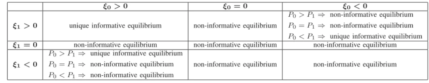
For the case where the encoder and the decoder have subjective priors on the source dis- tribution, under identical costs, we show that there exist fully informative Nash

uploaded them online for my colleagues and other teachers at the university to review. My findings revealed that much insight can be gained from the way in which

30-31 Ekim 1995’te Pekin’de yapılan Ulusal İhtisas Konferansı’nda; biyogübrelerin ürün verimini arttırdığı, toprak verimliliğini ve biyo-elverişliliğini