Month ahead rainfall forecasting using gene expression programming

http://www.aascit.org/journal/ees

Month Ahead Rainfall Forecasting Using Gene

Expression Programming

Ali Danandeh Mehr

Civil Engineering Department, Antalya Bilim University, Antalya, Turkey

Email address

Citation

A. Danandeh Mehr. Month Ahead Rainfall Forecasting Using Gene Expression Programming. American Journal of Earth and Environmental Sciences. Vol. 1, No. 2, 2018, pp. 63-70.

Received: February 20, 2018; Accepted: March 10, 2018; Published: April 10, 2018

Abstract: In the present study, gene expression programming (GEP) technique was used to develop one-month ahead monthly rainfall forecasting models in two meteorological stations located at a semi-arid region, Iran. GEP was trained and tested using total monthly rainfall (TMR) time series measured at the stations. Time lagged series of TMR samples having weak stationary state were used as inputs for the modeling. Performance of the best evolved models were compared with those of classic genetic programming (GP) and autoregressive state-space (ASS) approaches using coefficient of efficiency (R2) and root mean squared error measures. The results showed good performance (0.53<R2<0.56) for GEP models at testing period. In both stations, the best model evolved by GEP outperforms the GP and are significantly superior to the ASS models.

Keywords: Genetic Programming, Gene Expression Programming, Monthly Rainfall, Time Series Modelling, State-Space Modelling

1. Introduction

Monthly forecasts of rainfall are of paramount importance components of watershed planning for a number of reasons such as flood control, water allocation, irrigation policy, and drought management. However, precise forecast is not easily possible, owing to the highly random characteristics of rainfall events. Truthful forecasts of monthly rainfall is known as one of the specific challenges in stochastic hydrology. Classic time series modelling such as auto regressive (AR), AR integrated moving average (ARIMA) and seasonal ARIMA (SARIMA) have been used for monthly rainfall forecasting in earlier studies (Delleur and Kavvas 1978). Although these models are applied for stationary state of rainfall time series, they are basically linear models and have a limited ability to model rainfall time series in the presence of highly random features. They also cannot be used for generalization and have more limited performance in monthly rainfall forecasting (Nourani et al. 2009).

Recent studies have focused on the implementation of artificial intelligence (AI) methods, such as artificial neural network (ANN), Fuzzy logic (FL), support vector machine (SVM), for monthly rainfall forecasting (e.g., Aksoy and Dahamsheh 2009; Srivastava et al. 2010; Wu et al. 2010;

Abarghouei 2016). In spite of desired flexibility of AI models in rainfall forecasting, these studies have shown that the stand-alone AI mentioned methods cannot be successfully used to rainfall forecast, particularly in arid and semi-arid regions. Consequently, hybrid AI methods, such as wavelet-ANN, wavelet-ANFIS and wavelet-SVM, are being used nowadays. For example, Nourani et al. (2009) developed a WA-ANN coupled model for one-month ahead forecasting of Ligvanchai watershed precipitation at Tabriz, Iran and showed that the hybrid model can predict both short- and long-term precipitation events because of using multi-scale time series as the input layer.

Genetic Programming (GP), as a self-structuring system

identifier, has shown great ability in modelling and forecasting non-linear hydrologic time series in recent studies. Our review showed that only a few researchers have used GP for rainfall forecasting. List of the papers that applied a GP variant for this aim is presented in Table 1. For instance, gene expression programming (GEP) and hybrid wavelet-GEP conjunction (WGEP) models were developed to forecast daily rainfall series at two reengages located in the Aegean Region of Turkey (Kisi and Shiri 2011). The results indicated that WGEP model significantly improves efficiency of standalone GEP results. More recently, using large scale atmospheric circulation indices, ENSO and those from

tropical Indian Ocean (EQUINOO), Kashid and Maity demonstrated that GP can be satisfactorily used to predict monthly Indian Summer Monsoon Rainfall over India (Kashid and Maity 2012).

Auturegressive state-space (ASS) is a promising time and

spatial series analysis tool that has rarely been applied in raninfall forecasting, neither its comparison with other traditional AI methods. In the scenario of stationary data series, ASS is equivalent to the ARMA model (Shumway and Stoffer 2011). However, it assumes that the measurement vector is a linear transform of the true state vector with a white noise, and also it takes the measurement uncertainty into account. A filtering procedure is exists in ASS approach to deal with uncertainties, which in the meantime allows to analyze nonstationary data series and forecast values outside the measurement range (Morkoc et al. 1985; Nielsen and Wendroth 2003; Shumway and Stoffer 2011).

Table 1. Summary of the papers applied GP for rainfall forecasting.

Statistics

Authors GP variant Time scale

Bakhshaii and Stull (2007) GEP Daily

Kisi and Shiri (2011) GEP Daily

Kashid and Maity (2012) LGP Monthly

Dufek et al. (2017) GGP Daily

Danandeh Mehr et al. (2018) MGGP Monthly

To the best of the author’s knowledge, there is no study comparing different stand-alone GP and ASS methods for monthly rainfall forecasting so far. Thus, the goal of this study is to develop and compare two different GP variants, monolithic GP and GEP for monthly rainfall forecasting in two rain gage stations located at a semi-arid region, Iran. An ASS model is also developed for each rain gauge station as the benchmark. This is the first study that compares GEP and State space model for monthly rainfall forecasting so far.

2. Study Area and Observed Data

In the present study, GP-, GEP-, and ASS-based rainfall forecasting models are trained and tested using total monthly rainfall (TMR) time series measured at two rain gauge stations, Tabriz and Urmia, located in Urmia Lake basin a semi- aired area at Iran (Figure 1). The lake is the second largest saline lake in the world. However, it suffers from rapid decreasing in its water surface level these years, and

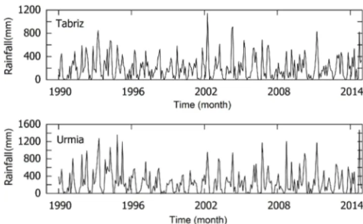
needs both local and regional attention to be treated. According to the basin climatology, mean annual rainfall is about 250 mm with a maximum rate commonly in spring months (March to May). Figure 2 shows 25 years (January 1990 to December 2014) of TMR time series at Tabriz and Urmia stations that were obtained from Iran Meteorological Organization (www.irimo.ir) and used in this study. The general information and the statistical properties of these stations are presented in Table 2. By considering location of the stations, it can be noticed that the western region of the lake receives more rainfall than its eastern region.

Figure 1. Location of Rain gauge stations used in the present study.

Figure 2. Observed rainfall data at Tabriz and Urmia Stations during 1990-2014 period.

Table 2. Geographic and descriptive statistics using the observations 1990, 01 – 2014.

Statistics

Meteor. Stations Latitude (°N)

Longitude (°E) Elevation (MSL) Min (mm) Max (mm) Mean (mm) Standard Deviation (mm) Tabriz 38.05 46.17 1345 0.00 1148.0 204.7 202.8 Urmia 37.40 45.03 1328 0.00 1475.0 257.2 282.7

3. Overview of GP, GEP, and ASS

Methods

GP (Koza 1990) is as the generalization of genetic

algorithm that was evolved mostly for system identification using automating programming technique. Thus, potential solutions (chromosomes) in GP are computer programs, however one can transform them to mathematical formulae if certain type of conditions is met. Chromosomes in standard

GP are represented by tree-shaped genes, which contains nodes and branches. Each node in the chromosome may contain a function or a terminal variable/constant. A set of primitive functions can encompass arithmetic operations, mathematical functions, Boolean operators or special functions for a given problem. Terminal set usually formed from input variables and random constants. Similar to the evolutionary process in genetic algorithm, the best solution is evolved through mating (reproduction, crossover, and mutation) of chromosomes within the GP population. Reproduction is asexual operation which means that only one chromosome is involved in the operation. It produces only one offspring, which is a pure copy of its parent. The process starts with the selection of the best chromosome from the population using a specified selection method, and completed by copying the chromosome without any variation into the new population (Danandeh Mehr et al. 2013). Crossover is another genetic operation, whereby two chromosomes (called parents) in the population produce two offspring consisting of genetic material of the parents. To this end, by defining the crossover point, each parent is divided into two parts, where the second part represents the subtree structure with crossover point as root node (Danandeh Mehr et al. 2017). Then, created subtrees are exchanged between parents. Eventually, mutation is another asexual operation that a parent is selected from the population and a node (mutation point) is replaced with a new subtree structure. The

generation of the subtree is similar as the generation tree structure in the initial population, except that the generation process in this case is controlled by the maximum operation level parameter (see Hrnjica and Danandeh Mehr 2018 for detail).

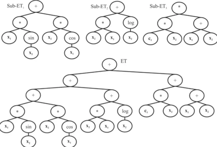
GEP is a certain type of multi-branch GP that allows the creation of expression trees (ETs; chromosome) containing one or multiple genes, each encoding a sub-expression tree (sub-ET), to solve a specific problem. In GEP, the output variable is computed by linking the relevant sub-ETs using algebraic or Boolean functions (AND, OR, NOT). In GP, computer programs (genes) follow the LISP language and are expressed as parse trees with different sizes and shapes. By contrast in GEP, the computer programs are considered as linear strings with fixed length composed of one or more genes. Each gene includes a head and tail. For the given number of genes g and length of head h, initial population of GEP chromosomes are created via filling the head and tail domains in respect to coding sequence of the genes known as open reading frame. An example of GEP individual involving three sub-expression trees (Sub_ET) were given in Figure 3. The evolution process in GEP is terminated when the GEP algorithm finds the perfect solution (the fitness of the best chromosome reaches specified value) or the specific number of generation is reached regardless of the quality of the solution. Details on GEP can be found in Ferriera (2002).

Like standard GP, the first step in GEP-based modelling is to generate an initial population of chromosomes (Danandeh Mehr and Demirel 2016). To this end, the modeler must specify primitive sets of terminals and functions. All possible predictors (parameters) can be defined as members of terminal set. Then, GEP identifies the most dominant predictors through its heuristic evolutionary optimization procedure. Primitive set of functions are typically selected via random selection or using the prior knowledge of the modeler about the problem at hand. To execute standard and GEP using monthly rainfall data, two software platforms, namely GpdotNetV4 (Hrnjica and Danandeh Mehr 2018) and GeneXproTool were used in the present study. While the former provides a free and open sources framework, the latter is a commercial package written in Java language.

Originally developed by Kalman and Bucy (1961), ASS initially used for filtering noise from aerospace-related and economic signals. Since the 1980s, its application has been extended to hydrology via analyzing the spatial associations among soil properties and crop performance (e.g., Wendroth et al., 1992, 2003; Cassel et al. 2000, Jia et al. 2017a;). However, it still remains unclear how it performs relative to rainfall forecasting and data-driven methods such as GP and GEP in estimating rainfall time series.

ASS forecasting models consists of a state equation and an observation equation (Shumway 1988). For the given time series Xi, the commonly used first-order state equation

describes the state vector Xi at time i with respect to the state

Xi-1 at previous time i-1:

Xi= α. Xi-1+ βi (1)

where α is the transition matrix and βi isthe uncorrelated

model error. Considering the measurement uncertainty in addition to the model error, the observation model relates the observed vector Yi to the true state vector Xi through a measurement matrix Mi and an uncorrelated measurement error matrix εi:

Yi-1= Mi. Xi-1+ εi (2)

The ASS models were solved with Kalman filtering and an iterative algorithm which terminated at the relative convergence limit of 0.005 (Shumway and Stoffer 1982). The optimal inputs for ASS model are selected via autocorrelation analysis of a given variable. The variables must normalize to the same order of magnitude prior to the state-space modeling.

In this case, the transition coefficient before each input variable actually describes its contribution to the output (estimate) in any state-space model. But it would not be sufficient when comparing the contributions of each variable in different models. The relative contribution of a particular variable was therefore calculated by dividing its transition coefficient by the sum of coefficients in each state-space model (Yang and Wendroth, 2014).

To evaluate the accuracy of the evolved models, coefficient of efficiency (R2) and root mean square error

(RMSE) measures are used in this study. The former is a normalized statistic showing how well the plot of observed data versus predicted data fits the 1:1 line. The latter is a quadratic scoring rule which measures the average magnitude of the error.

4. Results and Discussion

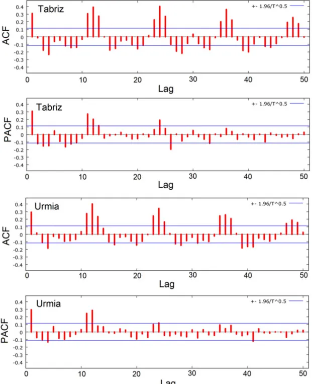
Identification of the optimal lag (input vectors) is an important task in time series modelling. Optimal set of lags may lead a model to create a parsimonious solution. By contrast, insufficient or redundant lags will produce poorly performing or highly complex models. Auto-correlation function (ACF) and/or partial ACF (PACF) are used in the identification of optimum lag in time series modelling. These are based on linear correlation between the present and past samples of a given time series. For the case of monthly rainfall time series, rainfall relation between successive months is not necessarily linear. Therefore, the approaches may lead quite large lags (uninformative variables) which is not necessarily required. To cope with the problem, this study has been benefited from both ACF/PACF analysis and evolutionary search algorithm existed in GP. To this end, firstly, we plot the correlogram of the TMR data and visually inspect the pattern of ACF and PACF (Figure 4). Then, GP/GEP was used in order to find the optimal set of lags. Figure 4 exhibits the ACF, PACF and the corresponding 95% confidence bands of TMR time series for the lag range of 0– 50 months in the stations. The ACF in both stations shows oscillating pattern with appearance of a sinusoidal function with a 12-month period (i.e., annual periodicity). This implies that total rainfall amount in a given month at each station is more correlated to its previous year amount than that of previous month. In addition, PACF in the stations shows more correlation between the current month rainfall and its antecedent values at lag-1, lag-11, lag-12 and lag-24, respectively. Therefore, 1-, 11-, 12-, 24-month lag are selected as the extent of lag implemented for an autoregressive monthly rainfall forecasting models in the stations.

(

)

f

R

R

R

R

R

=

,

,

,

,

ε

R

month t. The indices t-1 and t-11 are referred to as 1-month and 11-month lags, respectively and so on. εt is bias (noise)

term.

As discussed earlier, the ACF and PACF show the dependence from the perspective of linearity. There is no guarantee that input vectors given in Eq. (3) are optimal lags for a nonlinear predictive technique like GP/GEP. To determine the optimum number of lags, GP/GEP initially considers all the inputs equally important, then identifies optimal input vectors (dominant lags) through a trade-off among the input vectors. Thus, it is expected that the best solutions would contain only the most significant lags. In the

system identification process using soft computing methods, before data mining itself, a data pre-processing is applied to make input/output variables dimensionless and put them within a certain range. Moreover, these methods can remove nonstationary features of data. A specific type of data-processing approach suggested by Delleur and Kavvas (1978) was applied in the present study. To this end, the GP/GEP/ASS was trained and tested using TMR series after the series are square root transformed and then standardized so that they have zero mean and unit variance. It has been shown that subtracting the monthly means essentially removes the periodicity in the mean and in the variance and

yields a time series having weak stationary state which is satisfied for practical purposes (Delleur and Kavvas 1978). After data pre-processing, the first step to create the GP/GEP model is to determine the range of training and hold out unseen testing data sets. TMR series comprises 25 years records (see Figure 2). The first three years was separated to fill 24 lagged data for the period 1990-1992 (see Eq. 2). Therefore, the following 20 years (January of 1993 to December 2011) has been used to train the GP/MGGP. After producing the best GP/MGGP models for each station, separately, the models were tested against the hold out period 2012-2014.

Considering Eq. (2), four normalized rainfall series together with a set of random constants in the rage of [-2, 2] were chosen as members of the terminal set for both GP/MGGP runs in this study. Neglecting the complexity of evolved models, effect of various primitive functions with different probability of existence (i.e., weights of operation in the function set) is tested in order to find the best fitted model. The results showed that beside the basic arithmetic operations (+, -, ×, and /), trigonometric (including sin, cos, and tan) functions play very important roles in modelling. In addition, GP trails indicated that Half and Half initialization methods provided better results than Grow or Full initialization methods in this study. It should be mentioned

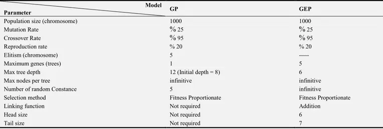
that RMSE was used as the fitness function to train both GP/GEP models in the present study. The average fitness simulation during each generation was monitored to stop the run in order to avoid over-fitting problem. The other parameters/methods used for GP and MGGP modelling setup have been listed in Table 3. As shown in the table, the mutation transform was applied with very high probability in this study. The reason behind is the fact that the models are dealing with very random and nonlinear data, and searching algorithm tends to converge very fast. To cope with the problem, choosing such high mutation rate would bring new genetic materials at each generation so that the modeler can achieve a population diversity as much as possible.

Table 3. The Parameter setting for the monolithic GP and MGGP runs 2009.

Model

Parameter GP GEP

Population size (chromosome) 1000 1000

Mutation Rate % 25 % 25

Crossover Rate % 95 % 95

Reproduction rate % 20 % 20

Elitism (chromosome) 5 ---

Maximum genes (trees) 1 5

Max tree depth 12 (Initial depth = 8) 6

Max nodes per tree infinitive infinitive

Number of random Constance 5 infinitive

Selection method Fitness Proportionate Fitness Proportionate

Linking function Not required Addition

Head size Not required 6

Tail size Not required 7

The efficiency results of the best evolved standard GP/GEP and ASS models at each station were presented in Table 4. It becomes obvious from Table 4 that rainfall was better forecasted with the GEP models than using GP or ASS modeling, regardless of the stations’ location. The probable reason is that GEP in contrast to the GP assumes different sub-ETs that might use each of them to capture a part of entire underlying process. The ASS model accounts for the temporal structure in the rainfall measurements provide the weakest efficiency. To be specific, a first-order autoregressive state-space used here, which is based on the autocorrelation of the present month rainfall and the

antecedent rainfall values, is not able to capture nonlinear characteristics between the output and input data.

Generally, the RMSE and R2 results are undesired, specifically during the test periods, if a high degree of precision is expected. The results indicated TMR forecast in the study region is difficult. Returning to the results of similar studies (e.g., Aksoy and Dahamsheh 2009; Abarghouei et al. 2016), the findings should not be considered as weak results. This reveals that additional attempts are inevitable to acquire better forecasts. One way to increase accuracy of the models might be implementation different data pre-processing techniques.

Table 4. Goodness of fit results of the models for monthly rainfall forecasting at stations.

Model Station Criterion

GP GEP ASS

Train Test Train Test

Tabriz RMSE (mm) 151.9 144.8 127.2 125.0 169 171 R2 _{0.460 0.409 0.622 0.560 0.33 0.29} Urmia RMSE (mm) 220 242 176 203 233 263 R2 0.392 0.302 0.613 0.530 0.321 0.175

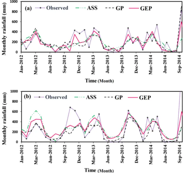
Figure 5 shows forecasted and observed TMR time series. It demonstrates all the models more or less are capable of capturing the oscillating pattern of the observed rainfall events, but they underestimate most of the high TMR

observations. The GEP model is more efficient in finding both local and global maxima compared to its counterparts. Although the GEP model significantly outperforms the others, the figure illustrates that the obtaining results are not

at the desired level of accuracy. There is still room for more studies to develop more precise models for long-term rainfall

forecasting in the study region.

Figure 5. Scatter diagram of rainfall forecasts at (a) Tabriz and (b) Urmia Stations.

5. Conclusions

In this study, the capability of standard GP, GEP, and ASS techniques were investigated for 1-months ahead monthly rainfall forecasting in Tabriz and Urmia stations, Iran. Weak stationary state of 1-, 11-, 12-, and 24-month lags of observed rainfall series were considered as inputs for the models. In general, the GEP modeling outperformed the GP and ASS method in estimating rainfall at both case study stations. However, the efficiency results showed that the models are not perfectly capable of forecasting the monthly rainfall series. Among the models, ASS approach was found as the least accurate one for at the stations. The reason for this behavior is probably caused by the fact that the relation between the rainfall and the antecedent values are far more than simply linear. In contrast to the GP and GP models, the ASS model assumes all the inputs are effective in the output value. This assumption is to some extent verified by the ACF

of rainfall which manifested significant autocorrelation coefficients at the first- 11-, 12- and 24-month lag. With respect to the best solution evolved by GEP. The best nonlinear formula does not necessary includes all the inputs. Thus, it can be concluded that ASS suffers from uninformative inputs that decrease the model efficiency.

Returning to the literature, it should be mentioned that neither ANN (Aksoy and Dahamsheh 2009) nor SVM (Feng et al. 2014) were able to forecast TMR values in arid regions with a desired level of accuracy. This results indicates the complexity of TMR forecasting in semi-arid to arid regions. The reason behind may rely on intermittent structure of the rainfall sequences as well as the high nonstationary feature of monthly rainfall series. Consequently, more complicated models such as hybrid models may need to develop truthful TMR forecasting models. Thus, developing hybrid wavelet-GP models might be a wisdom choice to improve the models examined in the present study.

References

[1] Abarghouei, H. B., Hosseini, S. Z. (2016), Using exogenous variables to improve precipitation predictions of ANNs in arid and hyper-arid climates. Arabian Journal of Geosciences, 9 (15), 663.

[2] Aksoy, H., Dahamsheh, A. (2009), Artificial neural network models for forecasting monthly precipitation in Jordan. Stochastic Environmental Research and Risk Assessment, 23 (7), 917-931.

[3] Cassel, D. K., Wendroth, O., Nielsen, D. R. (2000), Assessing spatial variability in an agricultural experiment station field: opportunities arising from spatial dependence. Agronomy Journal 92 (4), 706-714.

[4] Danandeh Mehr, A., Kahya E., Olyaie E. (2013), Streamflow prediction using linear genetic programming in comparison with a neuro-wavelet technique. Journal of Hydrology, 505: 240–249.

[5] Danandeh Mehr, A., Demirel, M. C. (2016), On the calibration of multigene genetic programming to simulate low flows in the Moselle river. Uludağ University Journal of The Faculty of Engineering, 21 (2), 365-376.

[6] Danandeh Mehr, A., Nourani, V., Hrnjica, B., Molajou A. (2017), A binary genetic programing model for teleconnection identification between global sea surface temperature and local maximum monthly rainfall events. Journal of Hydrology, 555, 397-506.

[7] Danandeh Mehr, A., Nourani, V., Karimi Khosroshahi,V., Ghorbani, M. A. (2018), A hybrid support vector regression-firefly model for monthly rainfall forecasting. International Journal of Environmental science and Technology, (accepted). [8] Delleur, J. W., Kavvas, M. L. (1978), Stochastic Models for

Monthly Rainfall Forecasting and Synthetic Generation. Journal of Applied Meteorology 17 (10), 1528-1536.

[9] Feng, Q., Wen, X., Li, J. (2015), Wavelet analysis-support vector machine coupled models for monthly rainfall forecasting in arid regions. Water resources management, 29 (4), 1049-1065.

[10] Ferreira C (2002), Gene expression programming in problem solving. In: Roy R et al (eds) Soft Computing and Industry, Springer, London, p 635–653.

[11] Hrnjica, B., Danandeh Mehr, A. (2018), Optimized genetic programming applications: emerging research and opportunities. IGI Global, DOI: 10.4018/978-1-5225-6005-0 [12] Jia, X., Shao, M., Zhu, Y., Luo, Y. (2017), Soil moisture

decline due to afforestation across the Loess Plateau, China. Journal of Hydrology 546, 113-122.

[13] Kalman, R. E., Bucy, R. S. (1961), New results in linear filtering and prediction theory. Journal of basic engineering. 83 (1), 95-108.

[14] Kisi, O., Shiri, J. (2011), Precipitation forecasting using wavelet-genetic programming and wavelet-neuro-fuzzy conjunction models. Water resources management, 25 (13), 3135-3152.

[15] Kashid, S. S., Maity, R. (2012), Prediction of monthly rainfall on homogeneous monsoon regions of India based on large scale circulation patterns using genetic programming. Journal of Hydrology, 454, 26-41.

[16] Koza J. R. (1992), The Genetic Programming Paradigm: Genetically Breeding Populations of Computer Programs to Solve Problems.

[17] Morkoc, F., Biggar, J. W., Miller, R. J., Nielsen, D. R. (1985), Statistical analysis of sorghum yield: A stochastic approach. Soil Science Society of America Journal 49 (6), 1342-1348. [18] Nielsen, D. R., Wendroth, O. (2003), Spatial and temporal

statistics: Sampling field soils and their vegetation. Catena, Reiskirchen, Germany.

[19] Nourani, V., Alami, M. T., Aminfar, M. H. (2009), A combined neural-wavelet model for prediction of Ligvanchai watershed precipitation. Engineering Applications of Artificial Intelligence, 22 (3), 466-472.

[20] Srivastava, G., Panda, S. N., Mondal, P., Liu, J. (2010), Forecasting of rainfall using ocean-atmospheric indices with a fuzzy neural technique. Journal of Hydrology, 395 (3-4), 190-198.

[21] Searson, D. P. (2015), GPTIPS 2: an open-source software platform for symbolic data mining. In Handbook of genetic programming applications (pp. 551-573). Springer, Cham. [22] Shumway, R. H., Stoffer, D. S. (2011), Time series analysis

and its applications, third ed. Springer, New York, USA. [23] Wendroth, O., Al-Omran, A. M., Kirda, C., Reichardt, K.,

Nielsen, D. R. (1992), State-space approach to spatial variability of crop yield. Soil Science Society of America Journal. 56, 801-807.

[24] Wendroth, O., Reuter, H. I., Kersebaum, K. C. (2003), Predicting yield of barley across a landscape: a state-space modeling approach. Journal of Hydrology, 272, 250-263. [25] Wu, C. L., Chau, K. W., Fan, C. (2010), Prediction of rainfall

time series using modular artificial neural networks coupled with data-preprocessing techniques. Journal of Hydrology, 389 (1-2), 146-167.