AGENCY COSTS, FISCAL POLICY, AND
BUSINESS CYCLE FLUCTUATIONS
A Master's Thesis
by
BURC_IN KISACIKOGLU
Department of
Economics
Bilkent University
Ankara
September 2009
AGENCY COSTS, FISCAL POLICY, AND
BUSINESS CYCLE FLUCTUATIONS
The Institute of Economics and Social Sciences of
Bilkent University
by
BURC_IN KISACIKOGLU
In Partial Ful llment of the Requirements For the Degree of MASTER OF ARTS in THE DEPARTMENT OF ECONOMICS B_ILKENT UNIVERSITY ANKARA September 2009
I certify that I have read this thesis and have found that it is fully adequate, in scope and in quality, as a thesis for the degree of Master of Arts in Economics.
||||||||||||||||||{ Assist. Prof. Dr. Refet S. G•urkaynak Supervisor
I certify that I have read this thesis and have found that it is fully adequate, in scope and in quality, as a thesis for the degree of Master of Arts in Economics.
|||||||||||||||||{ Assist. Prof. Dr. H. Cagr Saglam Examining Committee Member
I certify that I have read this thesis and have found that it is fully adequate, in scope and in quality, as a thesis for the degree of Master of Arts in Economics.
|||||||||||||| Assist. Prof. Dr. Ebru Voyvoda Examining Committee Member
Approval of the Institute of Economics and Social Sciences
||||||||| Prof. Dr. Erdal Erel Director
ABSTRACT
AGENCY COSTS, FISCAL POLICY, AND BUSINESS
CYCLE FLUCTUATIONS
KISACIKOGLU, Burcin M.A., Department of Economics Supervisor: Asst. Prof. Dr. Refet G•urkaynak
September 2009
This paper studies the relationship between scal policy, nancial market fric-tions and business cycle uctuations. It is shown that in an economy where balance sheets play a role in the propagation of shocks, using countercyclical scal policy net worth and output uctuations can be reduced. This counter-cyclical scal policy requires to distribute resources to the entrepreneurs when a negative technology shock is realized and levy taxes on entrepreneurs after the technology shock is back to zero. It is shown that after the realization of a negative shock, countercyclical scal policy reduces agency costs which would make entrepreneurs increase investment and dampen the business cycle uctu-ations via decreasing uctuuctu-ations in net worth. By this increase in investment, nancial fragility decreases, which reduces the slowdown of economic activity.
Keywords: Business Cycle Fluctuations, Agency Costs, Financial Accelerator, Countercyclical Fiscal Policy
•
OZET
TEMS_ILC_IL_IK MAL_IYETLER_I, MAL_IYE POL_IT_IKASI
VE KONJONKT •
UR DALGALANMALARI
KISACIKOGLU, Burcin Y•uksek Lisans, Ekonomi B•ol•um•u
Tez Y•oneticisi: Yrd. Doc. Dr. Refet G•urkaynak Eyl•ul 2009
Bu tez maliye politikas , nansal piyasa s•urt•unmeleri ve konjonkt•ur dalgalanmalar aras ndaki iliskiyi incelemektedir. Bilancolar n d ssal soklar n yay l m nda etkili oldugu ekonomilerde konjonkt•ur kars t maliye politikas kullan larak m•utesebbis •
ozvarl klar ve •uretimdeki dalgalanmalar n azalt labildigi g•osterilmistir. Bahsedilen konjonkt•ur kars t maliye politikas negatif teknoloji sokunun g•or•uld•ug•u zaman-larda m•utesebbislere kaynak aktar m n ve sokun s f ra geri d•ond•ug•u zamanlarda ise m•utesebbislerin vergilendirilmesini gerektirmektedir. Negatif teknoloji sokunun g•or•ulmesinden sonra konjonkt•ur kars t maliye politikas n n temsilcilik maliyet-lerinin d•usmesine neden olarak m•utesebbislerin yat r mlar n artt rd g g•or•ulm•ust•ur. Bununla beraber, konjonkt•ur kars t maliye politikas ile konjonkt•ur dalgalan-malar n n •ozvarl k dalgalanmalar yla beraber azalt ld g g•osterilmistir. Yat r mdaki bu art sla beraber ekonomik aktivitenin d•us•us•u azalt lm st r.
Anahtar Kelimeler: Konjonkt•ur Dalgalanmalar , Temsilcilik Maliyetleri, Finansal H zland r c , Konjonkt•ur Kars t Maliye Politikas
ACKNOWLEDGMENTS
I cannot overstate my gratitude to Assist. Prof. Dr. Refet G•urkaynak, for his guidance, advice, patience, support and showing me how to be a good economist. I would like to thank him for believing in me, pushing me to do the best I can and making me feel like I am a collegue rather than a student. I will always be indebted to him. I also would like to thank my examining committee members Assist. Prof. Dr. H•useyin Cagr Saglam and Assist. Prof. Dr. Ebru Voyvoda, for their helpful comments and suggestions. I thank my family for their encouragement, support and for being there when I needed them the most. Galip Kemal •Ozhan and _Ihsan Erman Saracgil, helped me get through these two years with their friendship and comments on the thesis. Finally, I would like to thank Elif Arslan for keeping me sane in my masters study. I would be lost without her.
TABLE OF CONTENTS
ABSTRACT . . . iii • OZET . . . iv ACKNOWLEDGMENTS . . . v TABLE OF CONTENTS . . . viLIST OF TABLES . . . vii
LIST OF FIGURES . . . viii
CHAPTER 1: INTRODUCTION . . . 1
CHAPTER 2: THE MODEL . . . 4
2.1 The Financial Contract . . . 6
2.2 Households and Firms . . . 9
2.3 Entrepreneurs . . . 11 2.4 Government Policy . . . 13 2.5 Equilibrium . . . 15 CHAPTER 3: SIMULATIONS . . . 17 3.1 Calibration . . . 17 3.2 Main Results . . . 18 CHAPTER 4: CONCLUSION . . . 24 BIBLIOGRAPHY . . . 26
LIST OF TABLES
1. Sequence of Events . . . 5
2. Parameter Values . . . 19
3. Maximum Percentage Deviations of the Benchmark Model . . . 20
LIST OF FIGURES
1. Impulse Responses of the Benchmark Model and the RBC Model . . . . 19 2. Impulse Responses of the Benchmark Model without Taxation and
CHAPTER 1
INTRODUCTION
Financial acclerator models incorporate nancial issues to the business cycle models, which the business cycle literature have largely ignored. According to these mod-els, nancial frictions are the reason of the long lived business uctuations which are costly. The purpose of this paper is to propose a stabilization policy under-taken by government via scal policy so that the e ects of the nancial frictions are reduced and uctuations are dampened. Government uses countercyclical scal policy (countercyclical in terms of transfer payments), i.e. government distributes transfer payments to entrepreneurs in bad times and levies tax on the pro ts of the entrepreneurs in good times to transfer resources to the nancially constrained entrepreneurs in bad times so that the nancial constraints can be eased.
For the students of business cycle research, the propagation mechanism behind the uctuations is an important question. In order to understand the propagation mechanism properly, starting with the seminal work of Kydland and Prescott (1982), microfounded business cycle models had been constructed. Eventhough these early attempts are seen to be important steps towards understanding the long lived re-sponses to shocks, it is shown by Cogley and Nason (1993, 1995) that the canonical real business cycle models could not replicate the hump-shaped behavior of the time series data due to the lack of internal propagation mechanism.
The poor performance of the real business cycle models against the time series data made economists to search for the models that could explain and replicate the long lived responses of the economy to the shocks. To investigate the role of
nancial market frictions in the business cycle propagation is the o spring of this search. These models incorporated the endogenous propagation mechanism through credit market, so that they could replicate the persistent movements in the data. Broadly these models show that the balance sheet conditions of the entrepreneurs are an important source of the propagation of shocks due to the agency costs arise from the nancial market imperfections. This class of models is named as nancial accelerator models.
A seminal contribution to this line of research was made by Bernanke and Gertler (1989). This study developed a simple neoclassical model of business cycle where the balance sheet of the entrepreneurs ampli es the upturn in good times and wors-ens the downturn in bad times. Following this study, Bernanke and Gertler (1990) showed that high agency costs decrease the amount and the e ciency of the invest-ment and this leads to nancial fragility. Gertler and Gilchrist (1994) empirically showed that the rms with di erent sizes are a ected di erently from the nancial market frictions. Carlstrom and Fuerst (1997) constructed a general equilibrium model with nancial market frictions and showed that nancial accelerator models can replicate the long lived responses observed in the time series.
The persistent uctuations generated by these models not only describe the world we live in, they also imply welfare costs for the consumers due to the uctuations in the consumption. Otrok (2001) shows that the welfare cost of business cycles can be as high as 40% of total consumption. Imrohoroglu (2008) points out that the economies with high consumption volatility has higher welfare costs. Since the uctuations in nancial accelerator models are highly persistent and ampli ed, one can expect the welfare costs to be high for this particular class of models.
The undesirability of the business cycle uctuations due to the welfare costs strenghtens the need for a stabilization policy in order to dampen the uctuations. If nancial accelerator models can describe the world correctly, the stabilization policy should take it into account. Then the goal of the stabilization policy should be to reduce the e ects of the frictions so that the uctuations can be less persistent
and dampened.
The results show that a simple scal scal policy rule can smooth the uctua-tions in entrepreneurs' net worth and lessen the output volatility, while respecting the government budget constraint. The government borrows from households in response to a negative technology shock, gives a transfer payment to entrepreneurs, who are taxed in the next period enough to ful ll the repayment obligation inclusive of the riskless interest rate. This turns out to be a boost for entrepeneurs because they e ectively get to borrow at the riskless rate via government at bad economic times, whereas they would have to pay a high external nance premium to bor-row directly. This interest rate subsidy increases investment and leads to a faster recovery of investors' net worth despite the subsequent tax burden.
The paper is organized as follows: Section 2 gives the details of the model, section 3 gives the impulse responses and we conclude in section 4.
CHAPTER 2
THE MODEL
The model utilized in this paper is a standard nonmonetary nancial accelerator model following Carlstrom and Fuerst (1997, 1998) with the inclusion of taxation. This is a general equilibrium model which includes entrepreneurs, households, gov-ernment, consumption good producing rms owned by households and nancial intermediaries as economic agents.
In the context of the model, entrepreneurs are investment good producing agents with low internal funds. To be able to undertake investment good produc-tion, they rely on external nancing supplied by the lenders, namely the house-holds. This borrowing made via nancial intermediaries (namely capital mutual funds) is typically limited since entrepreneurs do not have enough net worth to collateralize their debt. So lenders and entrepreneurs form a nancial contract that assumes costly state veri cation (CSV) which will be explained in detail in the next subsection. According to the nancial contract, the entrepreneur repays the contractual obligation if she can and bankrupts otherwise. The solvency of entrepreneurs are determined by the realized idisyncratic shocks to their projects: If the realized value of the shock is high enough, then they can repay their con-tractual obligations but otherwise they are bankrupt and their project returns are con scated by the lender. Since net worth is a collateral for the nancial contract, the contract implies that higher net worth leads to higher borrowing as a result higher investment and output. So uctuations in net worth will be an important determinant of the business cycle uctuations.
The undesirability of the uctuations makes room for the economic policy op-tions that can reduce the uctuaop-tions in the net worth and output. This paper will try to show that using scal policy tools, countercyclical transfer payments in this case, net worth uctuations can be dampened. So, also uctuations in investment and output will be reduced. Details of the scal policy will be explained in the further subsections.
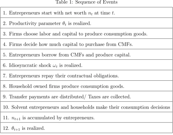
The sequence of events is given the table below: Table 1: Sequence of Events 1. Entrepreneurs start with net worth nt at time t:
2. Productivity parameter t is realized.
3. Firms choose labor and capital to produce consumption goods. 4. Firms decide how much capital to purchase from CMFs.
5. Entrepreneurs borrow from CMFs and produce capital. 6. Idiosyncratic shock !t is realized.
7. Entrepreneurs repay their contractual obligations. 8. Household owned rms produce consumption goods. 9. Transfer payments are distributed/ Taxes are collected.
10. Solvent entrepreneurs and households make their consumption decisions 11. nt+1 is accumulated by entrepreneurs.
12. t+1 is realized.
Since t is known at the begining of period t, there is no aggregate risk in
the economy and rms choose their labor and capital demand accordingly. To meet the demand of the rms and households, entrepreneurs borrows consumption goods from the CMFs and undertakes capital production. With the produced capital and supplied labor, rms produce consumption goods. After the production of the consumption goods the idiosyncratic shock !t is realized. Since CMFs
entrepreneurs declare bankruptcy and some repay their contractual obligations. Contingent on the realization of t, government either transfer payments to the
entrepreneurs or levy taxes on them after the contractual obligations are paid by the entrepreneurs. Finally solvent entrepreneurs and households make their consumption decisions.
2.1
The Financial Contract
In this subsection we consider the nancial contract in a partial equilibrium setting. This nancial contract generates an upward sloping supply curve for investment goods. General equilibrium issues a ect the contract through entrepreneurial net worth nt> 0 and through price of capital qt.
The nancial contract consists of two parties: entrepreneurs and lenders. En-trepreneurs have a su ciently small net worth nt> 0 and rely on external
nanc-ing for investment good production. Lenders provide external nancing to the entrepreneurs. Both agents are risk neutral.
The entrepreneur has access to a stochastic technology that transforms it
con-sumption goods into !tit units of capital, where !t is the idiosyncratic shock with
distribution , and characterized by density and mean unity. Agency costs are introduced to the model by assuming that the idiosyncratic shock ! is a private information for the entrepreneur and other agents can observe it at a cost of it
units of capital. This set-up is the one that is rst studied by Townsend (1979) and then by Gale and Hellwig (1985). They show that in such a CSV framework, the optimal contract is a standard debt contract where the borrower pays a xed rate if she can and default if she cannot in which case the lender con scates all the returns from the project.
The entrepreneur borrows (it nt) units of consumption goods and agrees to
repay 1 + rk
t (it nt) units of capital goods to the lender, where 1 + rtk is the
contractual interest rate. The entrepreneur defaults if the realization !tis less than
all returns from the project. If the realized value of !tis higher than the threshold
level, than the entrepreneur will repay the xed amount that is speci ed in the contract. The threshold level ! is therefore the value which equalizes the return from the project and the amount that is need to be repaid, i.e.
!tqtit = 1 + rtk (it nt)
!t =
1 + rkt (it nt)
qtit
.
where qt is the price of capital.
The optimal contract minimizes the incidence of costly monitoring. Therefore the nancial contract should be constructed in such a way that the entrepreneur should announce the true realization of !, because without monitoring, the asym-metric information creates moral hazard which would make the entrepreneur report failure of project to minimize payments. So the optimal contract is de ned on (i; !), where both of the arguments are common knowledge to all agents. The contract is made for one period, to side step the repeated game issues of the model1.
Under the contract, the expected entrepreneurial income is given by
qtitf (!t) = qtit
Z 1 !
!d (!) ! (1 (!t)) , (1)
where f (!t) is the fraction of expected net capital output received by the
en-trepreneur.
Entrepreneurs are taxed at rate t so the after tax pro ts of the entrepreneur
is,
(1 t) qtitf (!t) = (1 t) qtit
Z 1 !
! (d!) (1 (!t)) !t . (2)
1One can refer to Gertler (1992), for a theoretical analysis of an agency cost model with two
Similarly expected income of the lender on such a contract is given by, qtitg (!t) = qtit "Z ! 0 !d (!) (!t) + !t(1 (!t)) # ; (3)
where g (!t) is the fraction of the expected net capital output received by the
lender. The taxes are paid only by the entrepreneurs. Note that,
f (!t) + g (!t) = 1 (!t) : (4)
So on average, (!t) units of capital is destroyed by monitoring.
Now, the optimal contract is given by the (i; !) pair that maximizes the en-trepreneur's expected return subject to the lender being indi erent between loaning the funds and keeping them. So, the optimal contract is given by the solution to the following maximization problem,
max (1 t) qtitf (!t) subject to qtitg (!t) (it nt) : (5)
This constraint the lenders will lend their resources to the entrepreneurial ac-tivity. The participation constraint for the entrepreneurs, (1 t) qtitf (!t) nt
should also be satis ed. So the optimality conditions are,
qt = 1 1 (!t) + (!t) f(!t) f0(!t) (6) it = nt 1 qtg (!t) (7)
Equation (6) de nes an implicit function ! (qt), with ! increasing in qt. Using
equations (6) and (7) one can derive the aggregate investment supply function for the economy, which is Is(q; n) = i (q; n)f1 (!)g : This identity shows that aggregate investment depends only on price of capital, q, and aggregate en-trepreneurial net worth, nt. This observation will allow us to make inferences about
supply curve shifter, i.e. higher net worth decreases agency costs which boosts the capital production for a given price of capital. So net worth will be an important determinant of the changes in nancial fragility and output.
Multiplying both sides of equation (7) by (1 t) qtf (!t), we have
(1 t) qtitf (!t) =
(1 t) qtf (!t)
1 qtg (!t)
nt (8)
The coe cient qtf(!t)
1 qtg(!t) on nt is the expected return on internal funds of the
entrepreneur. This return must be greater than the riskless return, (1 + r), in order to make the entrepreneur to devote all of its resources to the investment good production. Otherwise, the entrepreneur would simply hold on to her resources and does not undertake the investment good production.
2.2
Households and Firms
The economy consists of a continuum of agents. The agents are of two types: entrepreneurs (fraction 1 ) and household (fraction ). As mentioned before the entrepreneurs produce the investment good. Entrepreneurs receive external nancing needed for production from households via intermediaries, namely the capital mutual funds (CMFs), which are assumed to be risk neutral. If a house-hold wishes to purchase capital, she must fund entrepreneurial projects, and these projects are subject to agency costs. Furthermore, CMFs take advantage of the law of large numbers by funding a large number of entrepreneurs to eliminate the idiosyncratic entrepreneurial uncertainty. So the households earn one unit of capi-tal with the expenditure of qt consumption goods, which is implied by the riskless
return of unity and they earn a risky return of qt 1 + rtk , if their funds are lended
to the entrepreneurs. The entrepeneurs will be borrowing the consumption goods from the CMFs which are supplied by the households. There are also consumer good producing rms, which are not subject to the agency costs. So we are not interested with their behavior.
Households are in nitely lived with the following utility function
U (ct; 1 ht) = ln (ct) + (1 ht)
The maximization problem of the household is
max E0 1 P t=0 t(ln (c t) + (1 ht)) ; 0 < < 1 (9)
subject to the budget constraint
wtht+ rtkht + (1 + rt) bt 1 bt+ ct+ qtit (10)
Here kh
t denotes the household stock of capital, ct denotes the household
con-sumption with its price assumed to be unity, htis the household labor rented to the
consumer good producing rms, wt labor wage, rt is the return on capital rented
to consumer good producing rms, bt is the government borrowing at the time t
from the households, qt is the price of capital and it is the investment.
The rst order conditions of the problem are,
qt=ct = Et
1 ct+1
[qt+1(1 ) + rt+1] (11)
ct = wt (12)
where is the depreciation rate.
The consumption good producing rms in this economy produce consumption goods by utilizing a constant returns to scale production function:
Yt= tKt (Ht)1 Hte (13)
where t is the stochastic productivity factor, Hte is the aggregate supply of
en-trepreneurial labor and Htis the aggregate supply of household labor. Competition
respec-tive marginal products. It is important to note that these rms are not subject to agency costs.
Finally t has the following stochastic dynamics:
t = (1 ) + t 1+ "t (14)
where "tis an i.i.d shock and is the nonstochastic steady state of the productivity
factor which is equal to 1.
2.3
Entrepreneurs
Now, we will focus on the entrepreneur behavior. In this setup, the entrepreneurs are long-lived. Furthermore, since the return on internal funds is greater than the riskless return, there is a possibility that they may postpone their consumption and accumulate enough funds to self- nance their production activities.2
Intro-ducing an additional discount factor, , makes entrepreneurs consume more than households in a given period3 and guarantees a nondegenerate lending equilibrium at all dates.
The maximization problem of the entrepreneur is,
max E0 1
P
t=0
( )tcet; 0 < < 1; 0 < < 1 (15)
subject to the budget constraint
(1 t) qtitf (!t) + xt cet+ qtzt+1 (16)
where, xt is the entrepreneurial wage, cet is the entrepreneurial consumption, zt is
the capital holdings of entrepreneur. Above constraint is derived by using equation
2Another reason of the possibility of fund accumulation is the linearity of the utility function
of the entrepreneur in consumption.
3Another modelling technique is to assume that the certain fraction of the entrepreneurs die
in each period and sell their accumulated capital stock to households. The modi ed version of the presented model can be found in Carlstrom and Fuerst (1996).
(8) and equation (19) which is the rule of motion for entrepreneurial capital, zt.
Solving this problem yields the following Euler equation,
qt= (1 t) Et f(1 ) qt+1+ rt+1g
qt+1f (!t+1)
1 qt+1g (!t+1)
(17) Note that if price of capital qt is set to 1, above Euler equation collapses to a
standard Euler equation. So one of the most important characteristic of the model is the endogenous determination of the price of capital.
To raise internal funds, the entrepreneur rents his capital and labor, which is inelastic, to the consumption good producing rms. After time t goods have been produced by the rms and households make consumption decisions, entrepreneurs sell their undepreciated capital to the nancial intermediary for the consump-tion goods in order to use them in investment good producconsump-tion. Furthermore en-trepreneurs receive transfer payments from government in case of a negative (below the mean) aggregate productivity shock is realized. After these transactions, the net worth of the entrepreneur is
nt = xt+ [rt+ qt(1 )] zt+ trt (18)
where rtis the return on capital, qt is the price of capital, zt is the entrepreneurial
capital, xtis the entrepreneurial wage and trtis the transfer payments received from
the government if a negative technology shock is realized at time t. Entrepreneurs use their net worth as a collateral for the nancial contract. They sell their capital in order to purchase consumption goods to undertake investment good production to CMFs.
Here the entrepreneurial wage, xt, is assumed to be small but positive so that
net worth is never zero. If the net worth is zero for any time period, then the entrepreneurs would not be able to borrow. As a result, optimal contract problem will not be well de ned.
net worth does not appear in the Euler equation meaning that it holds for all entrepreneurs either solvent or bankrupt. Using the budget constraint we can derive the rule of motion for the entrepreneurial capital, zt:
zt+1 = (1 t) f (!t) 1 qtg (!t) nt ce t qt (19)
2.4
Government Policy
Government raises revenue using proportional taxes levied on the pro ts of the entrepreneur and borrows from the households. For simplicity, the households are not subject to taxes. The revenues generated via taxation and borrowing made by the government are used to distribute transfer payments to the entrepreneurs when a negative aggregate productivity shock is realized and to repay the debt to the households.4 Again, the purpose of this paper is to show that countercyclical
scal policy rules can dampen the uctuations in the output, through reducing the uctuations in net worth without making any claims about the optimality or welfare improvement. One important point is that the ad hoc tax rules should satisfy the intertemporal budget constraint.
The intertemporal budget constraint for the government to be satis ed is as follows: 1 X t=0 trt (1 + r)t + (1 ) (1 + r) bt 1 1 X t=0 tqtitf (!t) (1 + r)t (20)
This intertemporal budget constraint implies that the present discounted value of tax revenues, P1
t=0
tqtitf(!t)
(1+r)t , should be greater or equal to the present discounted
value of the transfer payments, P1
t=0 trt
(1+r)t, and the repayment of loans from
house-holds, (1 ) (1 + r) bt 1. One important point to emphasize is only one period
borrowing is allowed for the government, i.e. government should repay the debt ac-crued next period after the borrowing. The above intertemporal budget constraint
4Note that, since entrepreneurial uncertanity is elminated by the capital mutual funds, only
is derived by using the following no-Ponzi condition:
lim
n!1
bt+n
(1 + r)t+n 1 = 0: (21)
Now the two period budget constraint can be written as follows5:
tqtitf (!t) + bt= trt+ (1 + r) bt 1: (22)
The idea behind the two period budget constraint is simple. Assume that government commits to a countercyclical policy rule such that it will distribute transfer payments to the entrepreneurs when a negative technology shock is realized and will not tax them until the shock returns to zero. Now assume that a negative aggregate productivity shock is realized at date t. Then at this period government should distribute transfer payments but do not have resources for the distribution due to the countercyclical scal rule. So government borrows from the households and distributes them to the entrepreneurs as transfer payments. Then in this case since tax revenues and debt repayment, (1 + r) bt 1, are zero and borrowing of the
government will be equal to the transfer payments, i.e. bt = trt for the period
t: However, government should repay the debt accrued at period t, next period. Since the technology shock will be zero, government will not distribute transfer payments but rather collect tax revenues to repay the debt. As a result, the tax revenues collected in period t + 1 will be used to repay the debt with the interest to the household, i.e. t+1qt+1it+1f (!t+1) = (1 + r)bt for t + 1. In short, government
will transfer resources to the entrepreneurs by borrowing from households at time t and chooses an appropriate tax rate to repay the debt at t + 1. Clearly this policy rule is a two period scal rule that satis es a two period budget constraint as well as the intertemporal budget constraint. Furthermore, we can independently pin down the values of bt and t using the budget constraint. This two period scal
5In this paper, is normalized to 0:5. This normalization has no e ect on the dynamics of
policy rule along with the budget constraint is useful and tractable in making inferences about the policy options.
Since we are considering state contingent scal rules, the transfer payments can be dependent on the aggregate productivity parameter, , under the implicit assumption that government can react to the aggregate productivity changes. This assumption is problematic since the aggregate productivity can be observed with a lag. So making the transfer payments contingent to the technology shock will be more appropriate for our purposes.
2.5
Equilibrium
This subsection will present the market clearing conditions and the competitive equilibrium of the model. Since there are two agents in the economy with di erent capital stocks, the total capital stock in the economy is
kt = zt+ (1 ) kth (23)
which has the rule of motion,
kt+1= (1 ) kt+ it[1 (!t) ] (24)
To close the model, we need to state the equilibrium conditions. There are four markets in the economy: a consumption goods market, a capital goods market and two labor markets. The clearing conditions are given by,
Ht = (1 ) ht (25)
Hte = (26)
Yt = (1 ) ct+ cet+ it+ qtitf (!t) + (1 ) ((1 + r) bt 1 bt) (27)
kt = zt+ (1 ) kht (28)
and entrepreneurs, respectively. Equation (27) is the consumption goods market clearing condition and equation (28) is the capital goods market clearing condition.
A recursive competitive equilibrium is de ned by decision rules for Kt+1, Zt+1,
Ht, qt, nt, it, !t, cet, ct, bt, t where the decision rules are stationary functions of
(Kt, Zt, t) and satisfy the following:
ct = (1 ) Yt Ht (29) qt=ct = Et 1 ct+1 qt+1(1 + ) + Yt+1 Kt+1 (30) kt+1 = (1 ) kt+ it[1 (!t) ] (31) qt = 1 1 (!t) + (!t) f(!t) f0(!t) (32) it = nt 1 qtg (!t) (33) nt = Yt He t + Yt Kt + qt(1 ) zt (34) zt+1 = (1 t) f (!t) 1 qg (!t) Yt He t + Yt Kt + qt(1 ) zt ce t qt (35) qt = Et (1 ) qt+1+ Yt+1 Kt+1 (1 t) qt+1f (!t+1) 1 qt+1g (!t+1) (36) Yt = (1 ) ct+ cet+ it+ qtitf (!t) + (1 ) ((1 + r) bt 1 bt) (37) bt = trt+ (1 + r) bt 1 tqtitf (!t) (38)
Equations (29) and (30) are labor supply decision and Euler equation for house-holds, respectively. Equation (31) is the rule of motion for aggregate capital. Equa-tions (32) and (33) are optimality condiEqua-tions from the optimal nancial contracting problem. Equations (34) and (35) are evolution of net worth and entrepreneurial capital, respectively. Equation (36) is the Euler equation for entrepreneurs. Equa-tion (37) is the two period government budget constraint and nally equaEqua-tion (38) goods market clearing condition.
CHAPTER 3
SIMULATIONS
This chapter will present the simulation results of the model and discuss them in detail. First of all, before going into the details of the simulation, we will explain how the parameters of the model are calibrated in the following section.
3.1
Calibration
The calibrations are consistent with Carlstrom and Fuerst (1997) and they roughly match their empirical counterparts. The constant v in the household utility func-tion is chosen so that steady state household labor supply, h, is 0:3. We set = 0:99 implying that steady state return on capital is around 4 percent annu-ally. The consumption production technology is Cobb-Douglas with capital share of 0:36, a household labor share of 0:6399, and an entrepreneurial labor share, , of 0:0001. Note that entrepreneurial labor share needs to be positive to ensure that entrepreneurs earn a positive amount of wage to make net worth positive at all dates. The depreciation rate, , is set to be equal to 0:025, is set to 0:95 as usual and is just a normalization which does not alter the conclusions of the paper. Following Carlstrom and Fuerst (1997) we set = 0:25.
The last two parameters, and , are calculated to match bankruptcy rate, (!), and the risk premium rate qt 1 + rk (1 + r) where qt 1 + rk is the risky
return to households and (1 + r) is the riskless rate which are calibrated for US. We set bankruptcy rate to 0:00974 quarterly and risk premium to 187 basis points
annually. So matching these calibrations, and are found to be 0:947 and 0:207, respectively. The values of the calibrated parameters are given in the table below.
Table 1: Parameter Values
v (!)
2:89 0:99 0:36 0:0001 0:025 0:5 0:25 0:00974 0:974 0:95
3.2
Main Results
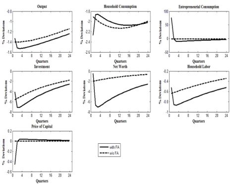
Now we will compute the impulse responses for the model with agency costs and for the model without agency costs ( = 0). The latter is essentially the canonical real business cycle model. The importance of this experiment is to be able make comparisons of the two models in terms of persistency and ampli cation of the shocks. Figure 1 below gives the impulse responses of output, entrepreneurial consumption, household consumption and labor, net worth, and investment to a one standard deviation negative technology shock.
In the above gure, dotted line represents impulses of the canonical real business cycle model and solid line represents the impulses of the nancial accelerator model. The dynamics of the real business cycle model is highly familiar. A negative aggregate productivity shock decreases the rental rate of capital and as a result investment decreases. As investment decreases, output and net worth falls. So both households and entrepreneurs reduce their consumption.1 Since = 0 for
the real business cycle model, it implies that price of capital is equal to 1, so we do not see any deviation in the price of capital. Finally variables move to their steady state as productivity starts picking up towards its steady state.
However, in the agency cost model the dynamics are quite di erent. The im-pulses exhibit hump-shaped responses observed in the time series but not in the canonical real business cycle model due to the missing internal propagation mech-anism. The reason behind the hump-shapes in the responses can be explained by the behavior of the net worth. As the negative shock hits the economy, it decreases the entrepreneurial wage and rental income. As a result, the net worth decreases slightly with the impact. Then investment decreases as net worth decreases, which decreases the price of capital. By the decrease in the investment, entrepreneurial consumption increases since entrepreneurs allocate their resources to consumption. Moreover, the decrease in investment decreases the entrepreneurial capital. So this has a direct e ect on the net worth, which decreases further. The output also shows the hump-shaped dynamics as in investment and net worth.
The maximum percentage deviations of household consumption, investment, entrepreneurial consumption, net worth, price of capital and output from their steady state values are given in the table below for the benchmark model:
Table 2: Maximum Percentage Deviations of the Benchmark Model H. Cons. Ent. Cons Inv. Net Worth P. of Cap. Output
2:27% 76:9% 7:1% 7:06% 0:46% 1:53%
1The decline in the entrepreneurial consumption is about 2%, but since the spike in the agency
cost model is extremely high we do not see the deviation of entrepeneurial consumption for the RBC model.
In this model the accelerator mechanism is at work: An adverse shock to the economy reduces the price of capital and the net worth of the nancially con-strained entrepreneurs. Since the entrepreneurs cannot nd enough funds to un-dertake investment due to the agency costs, both investment and output fall which leads to the further reduction of the net worth. That leads to a persistent and am-pli ed slowdown of economic activity. These persistent and amam-pli ed responses are highly cosistent with the time series data. This is the reason why this class of models are attractive for the business cycle students.
Next simulation will introduce a procyclical taxation rule with countercyclical transfer payments, which reduces the net worth uctuations. The countercycli-cality of the transfer payments is important since the government will subsidize the entrepreneurs when a below the mean aggregate productivity shock is realized. Consider the transfer payment rule, which government subsidizes the entrepreneurs by "t0:4 when an adverse shock or below the mean aggregate productivity shock, hits the economy. This rule has the implicit assumption that the government can respond to the technology shocks. It is important once again to point out that the tax rule should satisfy the two period budget constraint. Government will borrow from the households as much as the amount of the transfer payment in the period of the negative productivity shock is realized and tax revenue will be zero for this period. In the next period, government should repay the debt with interest to the households. This repayment will be covered by the tax revenues, since the technology shocks are one period in length.
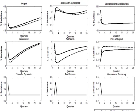
Figure 2 below gives the impulse responses of the benchmark model without taxation and with taxation to the same negative technology shock studied in gure 1:
Figure 2: Impulse Responses of the Benchmark Model without Taxation and with Taxation
In the above gure the solid line represents the impulses of the benchmark model with taxation and dotted line represents the impulses of the benchmark model without taxation. First thing to notice is that scal policy can signi cantly dampen the uctuations caused by the nancial market frictions. When the neg-ative technology shock is realized, it a ects net worth through reduction in the entrepreneurial wage. But this initial decrease in net worth is dampened by the transfer payments distributed by the government in the period of the shock. This dampened decrease in net worth also reduces the initial fall in the investment rel-ative to the benchmark model. As a result, price of capital decreases less and entrepreneurial consumption increases less in the period of the shock. Finally out-put falls less than the benchmark case. Since a negative shock is realized, tax revenue is zero in the rst period.
However in the second period, after the shock is back to zero, government levies tax on the pro ts of the entrepreneurial projects in order to repay the debt to the households, since government is allowed to borrow only for one period. As tax revenue increases, net worth falls further since it is still below the steady state level. This decrease makes investment decrease even more but not as much as the benchmark model without taxation. As a result price of capital stays below the steady state level and picks up slowly. This further decrease of net worth and investment makes output fall further, but still staying above the benchmark model and exhibiting a hump-shaped response. Then economy starts pick up to the steady state levels with tax revenue going to zero.
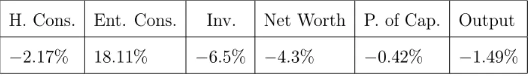
The maximum percentage deviations of household consumption, investment, entrepreneurial consumption, net worth, price of capital and output from their steady state values are given in the table below for the nancial accelerator model with taxation is as follows:
Table 3: Maximum Percentage Deviations of the BM with Taxation H. Cons. Ent. Cons. Inv. Net Worth P. of Cap. Output
2:17% 18:11% 6:5% 4:3% 0:42% 1:49%
When a procyclical taxation rule is introduced, the uctuations are dampened. Moreover, the hump-shaped responses of the variables are preserved by the be-havior of the net worth. A one time negative productivity shock increases the transfer payments, since transfer payments are countercyclical. Transfer payments distributed by the government makes net worth decrease less and helps net worth to pick up more quickly. This reduced decrease in net worth makes agency costs in-crease less relative to the benchmark model. So the entrepreneurs can bene t more from the investment opportunities. Eventhough decrease in rental capital decreases investment demand, a smaller decrease in net worth, smaller increase in borrowing rates makes entrepreneurs undertake investment projects, which dampens the
de-crease in the investment demand as well as in the inde-crease in the entrepreneurial consumption. As a result, the price of capital and the entrepreneurial capital de-creases less. Since the uctuations in the net worth and investment are dampened, output decreases less.
Another important result of the model is about persistence of uctuations. Since transfer payments to entrepreneurs decreases the e ects of nancial market imperfections by preventing agency costs to increase a lot, the uctuations in net worth become less persistent. As a result, investment and output reach their steady state in a shorter period of time compared to the benchmark model. Furthermore, by reducing the uctuations in net worth and entrepreneurial consumption we can say that scal policy has a positive impact on the welfare of the entrepreneurs. By reducing the consumption uctuations, welfare cost of business cycle decreases since entrepreneurs can smooth out their consumption path.
CHAPTER 4
CONCLUSION
This paper extended a simple real business cycle model where scal policy has a role in the business cycle uctuations due to the nancial frictions. The critical insight is that distributing transfer payments dampens the decrease in net worth, which decreases the uctuations in investment and output. As a result, agency costs increase less due to the smaller fall in the net worth and entrepreneurs can bene t more from the investment opportunities and vice versa in good times. Furthermore, as the e ects of nancial frictions are reduced with the fall in the agency costs, the uctuations become less persistent. These results re-emphasize in the importance of economic policy in times of nancial distress. A countercyclical scal policy in terms of transfer payments, can reduce nancial distress by making the balance sheets less vulnerable to nancial market conditions and to the adverse productivity shock.
One important point to emphasize is that this paper did not talk about whether the tax rule is optimal or welfare improving. If we were dealing with lump-sum taxation, then any tax that reduces the uctuations are to be welfare improving, since the steady state is not distorted. For this model we are dealing with a distorted steady state, which makes the answer of the welfare question is non-trivial. The next step is, obviously, to derive the welfare criterion for the agents and to try to nd a welfare improving tax rule, or directly solve the Ramsey problem to nd the optimal taxation. While most of the optimal taxation problems only have
households as a taxed agent, this model will need some non-trivial modi cations since there are heterogenous agents present.
26
BIBLIOGRAPHY
Bernanke, Ben S., and Mark Gertler. 1989. “Agency Costs, Net Worth, and Business Fluctuations,” American Economic Review 79(March): 14-31
Bernanke, Ben S., and Mark Gertler. 1990. “Financial Fragility and Economic Performance,” The Quarterly Journal of Economics 105(Feb.): 87-114.
Bernanke, Ben S., Mark Gertler, and Simon Gilchrist. 1996. “The Financial Accelerator and Flight to Quality,” Review of Economics and Statistics 78(Feb.): 1-15.
Bernanke, Ben S., Mark Gertler, and Simon Gilchrist. 1999. “The Financial Accelerator in a Quantitative Business Cycle Framework”. In J. Taylor and M. Woodford, eds Handbook of Macroeconomics, Vol. 1C.. Amsterdam: Elsevier, pp. 1341-1393.
Carlstrom, Charles. T., and Timothy S. Fuerst. 1996. “Agency Costs, Net Worth, and Business Fluctuations: A Computable General Equilibrium Analysis,” Working Paper No: 9602. Federal Reserve Bank of Cleveland.
Carlstrom, Charles. T., and Timothy S. Fuerst. 1997. “Agency Costs, Net Worth, and Business Fluctuations: A Computable General Equilibrium Analysis,” American
Economic Review 87(December): 893-910.
Carlstrom, Charles T., and Timothy S. Fuerst. 1998. “Agency Costs and Business Cycles,” Economic Theory 12: 583-597.
Cogley, Timothy, and James M. Nason. 1993. “Impulse Dynamics and Propagation Mechanisms in a Real Business Cycle Model,” Economics Letters 43(1): 77-81. Cogley, Timothy, and James M. Nason. 1995. “Output Dynamics in Real Business
Cycle Models,” American Economic Review 83(3): 492-551.
Gale, Douglas, and Martin Hellwig. 1985. “Incentive Compatible Debt Contracts I: The One Period Problem,” Review of Economic Studies 52(Oct.): 647-64.
27
İmrohoroğlu, A. 2008. “Welfare Costs of Business Cycles,” Steven Durlauf and Lawrance Blume eds. The New Palgrave Dictionary of Economics Second Edition 2009, Palgrave Macmillan
King, Robert G., Charles I. Plosser, and Sergio T. Rebelo. 1988. “Production, Growth, and Business Cycles: I. The Basic Neoclassical Model,” Journal of
Monetary Economics 21(May): 195-232.
Kiyotaki, Nabuhuro, and John. H. Moore. 1997. “Credit Cycles,” Journal of Political
Economy 105(2): 211-248.
Kydland, Finn E., Edward C. Prescott. 1982. “Aggregate Fluctuations and Time to Build,” Econometrica 50(6): 1345-1370.
Mayer, Eric, and Oliver Grimm (2008). "Countercyclical Fiscal Policy, Simple Rules, and Price Dispersion," Working Paper. Würzburg, Germany: University of Würzburg.
Modigliani, Franco, and Merton Miller. 1958. “The Cost of Capital, Corporation Finance, and the Theory of Investment,” American Economic Review 48(3): 261-297.
Otrok, Christopher. 2001. “On Measuring Welfare Cost of Business Cycles,” Journal
of Monetary Economics 47(2001): 61-92.
Schmitt-Grohé Stephanie, and Martin Uribe. 2007. “Optimal Simple and Implementable Monetary and Fiscal Rules” Journal of Monetary Economics 54(2007): 1702-1725.
Peréz, Javier J., and Paul Hiebert. 2004. “Identifying Endogenous Fiscal Policy Rules for Macroeconomic Models,” Journal of Policy Modelling 26(July): 1073-1089.
Townsend, Robert M. 1979. “Optimal Contracts and Competitive Markets with Costly State Verification,” Journal of Economic Theory 21(Oct): 265-96.