HIERARCHY PROCESS
a thesis
submitted to the department of industrial engineering
and the institute of engineering and science
of bilkent university
in partial fulfillment of the requirements
for the degree of
master of science
By
Mehmet Tun¸c
July, 2004
Prof. Dr. ¨Ulk¨u G¨urler (Supervisor)
I certify that I have read this thesis and that in my opinion it is fully adequate, in scope and in quality, as a thesis for the degree of Master of Science.
Asst. Prof. Dr. Oya Ekin Kara¸san
I certify that I have read this thesis and that in my opinion it is fully adequate, in scope and in quality, as a thesis for the degree of Master of Science.
Asst. Prof. Dr. Yavuz G¨unalay
Approved for the Institute of Engineering and Science:
Prof. Dr. Mehmet B. Baray
Director of the Institute Engineering and Science
BY USING THE ANALYTIC HIERARCHY PROCESS
Mehmet Tun¸cM.S. in Industrial Engineering Supervisor: Prof. Dr. ¨Ulk¨u G¨urler
July, 2004
Due to imprecision or uncertainty that is inherent in the design process, the management of research and development projects is very challenging. With the growing complexity of the design process and need for different specializations, it is getting even more tougher. Especially, in an organization where tens of high-tech, military R&D projects are carried out concurrently, management should be supported with the state-of-the-art decision and operations research methods.
In this thesis, we consider an application of the classification of R&D projects. More specifically, the problem discussed in this study is grouping N different projects into groups based on a predetermined set of features. Since some fea-tures are fuzzy, expert knowledge is needed to quantify the feafea-tures. In order to quantify the features successfully, Analytic Hierarchy Process is used. Finally, by using various clustering algorithms the projects are clustered.
Keywords: Analytic Hierarchy Process, clustering projects, quantification,
multi-criteria clustering, project evaluation. iii
ANAL˙IT˙IK H˙IYERARS¸˙I Y ¨
ONTEM˙IN˙I KULLANARAK
AR&GE PROJELER˙IN˙IN SINIFLANDIRILMA
UYGULAMASI
Mehmet Tun¸cEnd¨ustri M¨uhendisli˘gi, Y¨uksek Lisans Tez Y¨oneticisi: Prof. Dr. ¨Ulk¨u G¨urler
Temmuz, 2004
Tasarım s¨urecinin do˘gasından kaynaklanan belirsizlikler sebebiyle, ara¸stırma ve geli¸stirme projelerinin y¨onetimi olduk¸ca zordur. Tasarım ¸calı¸smalarının artmakta olan karma¸sıklı˘gı ve farklı alan uzmanlıkları gereksinimi y¨onetilmelerini daha da zorla¸stırmaktadır. ¨Ozellikle, onlarca y¨uksek teknoloji i¸ceren askeri Ar-Ge pro-jelerinin bir arada y¨onetildi˘gi bir organizasyonda y¨onetimin, modern karar verme ve y¨oneylem ara¸stırması y¨ontemleri ile desteklenmesi gerekmektedir.
Bu tezde, Ar-Ge projelerinin sınıflandırılmasına ili¸skin bir uygulama ince-lenmi¸stir. Bu ¸calı¸smada anlatılmakta olan problem, N farklı projenin ¨onceden belirlenmi¸s nitelik seti temel alınarak sınıflandırılmasıdır. Bazı niteliklerin belir-siz olması sebebiyle bu niteliklerin ¨ol¸c¨umlerinde uzman bilgisine ihtiya¸c duyul-maktadır. Bu nitelikleri ba¸sarıyla ¨ol¸cmek i¸cin bu ¸calı¸smada “Analitik Hiy-erar¸si Y¨ontemi” kullanılmı¸stır. Son olarak nitelikleri ¨ol¸c¨ulm¨u¸s projeler ¸ce¸sitli sınıflandırma y¨ontemleri kullanılarak sınıflandırılmı¸slardır.
Anahtar s¨ozc¨ukler : Analitik Hiyerar¸si Y¨ontemi, proje sınıflandırma, nice-lendirme, ¸coklu kriter sınıflandırma, proje de˘gerlendirme.
I am very grateful firstly to my thesis advisor, Prof. Dr. ¨Ulk¨u G¨urler for her patience, encouragement, guidance in my thesis work. I am indebted to other respected members of the thesis committee, Asst. Prof. Dr. Oya Ekin Kara¸san and Asst. Prof. Dr. Yavuz G¨unalay for accepting to read and review this thesis and for their suggestions. Thanks to their invaluable contribution, I have managed to complete my thesis work.
I would like to express my sincere thanks and gratitude to my manager at Aselsan, Ms. Elif Baktır. It would be impossible for me to complete my thesis work without her understanding, support, and motivation.
I would like to thank my colleagues, Onur Kabul, Aybeniz Yi˘git, and Aykut ¨
Ozsoy at Aselsan for their support, friendship, suggestions during all Aselsan time. I also wish to express my thanks to MST (Microwave and System Tech-nologies), one of the three divisions of Aselsan.
I would like to take this opportunity to thank Meray Y. ˙Ilhan for her help, support and love, especially during this thesis completion process.
I would also express my gratitude to mom, dad, my brother H¨useyin for their understanding, support, and most importantly for their love.
1 Introduction 1
1.1 Motivation . . . 1
1.2 Organization of the Thesis . . . 2
2 Related Work 3 2.1 Project Classification . . . 3
2.2 Analytic Hierarchy Process (AHP) . . . 4
2.2.1 Theoretical Structure of AHP . . . 5
2.2.2 AHP Methodology . . . 6
2.2.3 Pairwise Comparisons . . . 7
2.2.4 Group Process . . . 9
2.2.5 Deriving Relative Weights . . . 11
2.2.6 Checking Consistency of the Results . . . 11
2.2.7 Synthesis of Priorities . . . 14
2.2.8 A Numerical Example . . . 14
2.2.9 Criticisms of AHP and a Variant of AHP . . . 19
2.3 Multicriteria Clustering . . . 20
2.3.1 AHP Based Clustering . . . 20
2.3.2 VAHP Based Clustering . . . 24
2.3.3 An extension of the k-means algorithm . . . 24
2.3.4 General Clustering Algorithms . . . 25
3 Model and The Analysis 28 3.1 Defining The Projects In Terms of Features . . . 29
3.1.1 Features . . . 29
3.1.2 AHP Model . . . 33
3.2 Clustering The Projects . . . 37
4 Application of Project Clustering 39 4.1 Application of AHP . . . 42
4.1.1 Evaluation of Features . . . 42
4.1.2 Evaluation of Projects . . . 43
4.2 Application of VAHP . . . 44
4.3 Application of Clustering Algorithms . . . 46
4.3.1 AHP Based Clustering . . . 47
4.3.2 VAHP Based Clustering . . . 54 4.3.3 Extension of K-means Algorithm for Multicriteria Clustering 56
4.4 Investigation of Project Clusters . . . 56
5 Conclusions and Future Work 59
A Input Data: Pairwise Comparisons 61
2.1 Combined Judgments . . . 10
2.2 Hierarchical Structure of Numerical Example . . . 16
2.3 A Matrix for Criterion ‘Hardware Expandability’ . . . 16
2.4 A Matrix and Priority Vector for Objective . . . 16
2.5 A Matrix and Priority Vector for Criterion ‘Hardware Maintain-ability’ . . . 17
2.6 A Matrix and Priority Vector for Criterion ‘Financing Available’ 17 2.7 A Matrix and Priority Vector for Criterion ‘User Friendly’ . . . . 17
2.8 Decision Matrix and Solution of Numerical Example . . . 18
2.9 Hierarchy of the AHP Model in Ben-Arieh and Triantaphyllou’s Work . . . 23
3.1 Hierarchical Structure . . . 35
4.1 ProTer . . . 41
4.2 Matrix-Based Clustering: Use of Hierarchical Clustering Algorithm 49 4.3 Matrix-Based Clustering: Silhouette Graph for k = 5 . . . . 50
4.4 Aggregate-value Clustering: Use of Hierarchical Clustering Algo-rithm . . . 52 4.5 Aggregate-value Clustering: Silhouette Graph for k = 4 . . . 53 4.6 VAHP Based Clustering: Use of Hierarchical Clustering Algorithm 55 4.7 VAHP Based Clustering: Silhouette Graph for k = 5 . . . . 55
A.1 Evaluation of Features by Pairwise Comparisons: Matrix A of Ex-pert 1 . . . 61 A.2 Evaluation of Features by Pairwise Comparisons: Matrix A of
Ex-pert 2 . . . 62 A.3 Evaluation of Features by Pairwise Comparisons: Matrix A of
Ex-pert 3 . . . 62 A.4 Evaluation of Features by Pairwise Comparisons: Matrix A of
Ex-pert 4 . . . 62 A.5 Evaluation of Projects by Pairwise Comparisons With Respect to
”Technological Uncertainty”: Matrix A of Expert 1 . . . 63 A.6 Evaluation of Projects by Pairwise Comparisons With Respect to
”Technological Uncertainty”: Matrix A of Expert 2 . . . 64 A.7 Evaluation of Projects by Pairwise Comparisons With Respect to
”Technological Uncertainty”: Matrix A of Expert 3 . . . 65 A.8 Evaluation of Projects by Pairwise Comparisons With Respect to
”Technological Uncertainty”: Matrix A of Expert 4 . . . 66 A.9 Evaluation of Projects by Pairwise Comparisons With Respect to
A.10 Evaluation of Projects by Pairwise Comparisons With Respect to ”Platform Type”: Matrix A of Expert 2 . . . 68 A.11 Evaluation of Projects by Pairwise Comparisons With Respect to
”Platform Type”: Matrix A of Expert 3 . . . 69 A.12 Evaluation of Projects by Pairwise Comparisons With Respect to
”Platform Type”: Matrix A of Expert 4 . . . 70 A.13 Evaluation of Projects by Pairwise Comparisons With Respect to
”Work and Test Environment”: Matrix A of Expert 1 . . . 71 A.14 Evaluation of Projects by Pairwise Comparisons With Respect to
”Work and Test Environment”: Matrix A of Expert 2 . . . 72 A.15 Evaluation of Projects by Pairwise Comparisons With Respect to
”Work and Test Environment”: Matrix A of Expert 3 . . . 73 A.16 Evaluation of Projects by Pairwise Comparisons With Respect to
”Work and Test Environment”: Matrix A of Expert 4 . . . 74 A.17 Evaluation of Projects by Pairwise Comparisons With Respect to
”System Scope”: Matrix A of Expert 1 . . . 75 A.18 Evaluation of Projects by Pairwise Comparisons With Respect to
”System Scope”: Matrix A of Expert 2 . . . 76 A.19 Evaluation of Projects by Pairwise Comparisons With Respect to
”System Scope”: Matrix A of Expert 3 . . . 77 A.20 Evaluation of Projects by Pairwise Comparisons With Respect to
”System Scope”: Matrix A of Expert 4 . . . 78
2.1 Scale of Relative Importance . . . 8
2.2 Random Indices (RI)[13] . . . 13
2.3 Membership Table . . . 22
3.1 Output Table . . . 36
4.1 Features’ Weights . . . 43
4.2 Projects’ Weights for Subjective Features . . . 44
4.3 Projects’ Weights for Objective Feature . . . 45
4.4 Output Table of AHP . . . 45
4.5 Output Table of VAHP . . . 46
4.6 Matrix-Based Clustering: Use of K-means Clustering Algorithm (k = 7) . . . . 49
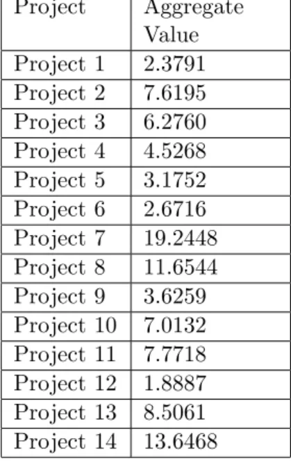
4.7 Aggregate-value Clustering: Input Data . . . 51
4.8 Aggregate-value Clustering: Use of K-means Clustering Algorithm (k = 4) . . . . 52
4.9 VAHP Based Clustering: Use of K-means Clustering Algorithm (k = 5) . . . . 54 4.10 Projects’ Rankings . . . 56 4.11 Extension of K-means Algorithm for Multicriteria Clustering (k = 5) 57
Introduction
Due to imprecision or uncertainty that is inherent in the design process, the management of research and development projects is very challenging. With the growing complexity of the design process and need for different specializations, it is getting even more complicated. Especially, in an organization where tens of high-tech, military R&D projects are carried out concurrently, management should be supported with the state-of-the-art decision making and operations research methods.
1.1
Motivation
Aselsan A.S¸. is one of the biggest companies in the military electronics sector in Turkey. MST (Microwave and System Technologies) is one of the three di-visions of Aselsan. In MST, there is a project-based structure, and it is one of the examples of organizations where tens of high-tech military R&D projects are carried out concurrently. As it is the case in MST, the projects may have completely different characteristics. For example, in terms of design type, some projects require breakthrough design, whereas some others require just redesign or continuous design of previously designed systems. Hence, the ways that each of the projects are managed and treated, may/should differ.
In this thesis, our aim is to form meaningful project clusters based on project characteristics. In other words, the objective is to identify project groups with common characteristics so that they can be managed in similar manners. This work can be thought as the first step of determining key issues for administrative processes of projects having same characteristics.
The features of projects have been determined beforehand for the case of MST, and the question of what should be the features of R&D projects, is not addressed in this thesis. The key point in this work is defining the projects in terms of features, and measuring the amount of each of the features that each project possesses. Some features are fuzzy, some others are not fuzzy, but their effects to project management are fuzzy. Therefore, expert knowledge is the main source. For this reason, Analytic Hierarchy Process (AHP) is used to define the projects in terms of features.
1.2
Organization of the Thesis
The thesis is organized as follows: Chapter 2 summarizes the studies in the literature on project classification, Analytic Hierarchy Process and multicriteria clustering. In Chapter 3, the model, constructed for the clustering of projects, is explained. Chapter 4 includes the application part of the study. Finally, Chapter 5 concludes the thesis.
Related Work
2.1
Project Classification
A frequently used process by which products are created is the practice of project management. In fact, projects have become one of the most common forms of temporary organizations, and they are set for achieving a wide variety of organi-zational goals. Yet, ironically, as an organiorgani-zational concept, project management is relatively new and probably not well understood. Most research literature on the management of projects is relatively inchoate and still suffers from a scanty theoretical basis and a lack of concepts [18].
One of the major barriers in understanding the nature of projects has been the little distinction made between the project type and its strategic and managerial problems. According to Pinto and Covin(1989) [12] “The prevailing tendency among the majority of academics has been to characterize all projects as funda-mentally similar, and the implicit view of many academics could be represented by the axiom, a project is a project.” However, works related to some distinc-tions among projects, based on levels change, exists (Blake (1978) [4], Hauptman (1986) [7], Whellwright and Clark(1992) [21], Shenhar(2001) [18]). Shenhar [18] noted that none of the typologies mentioned in the literature has developed into
a standard, fully accepted theoretical framework. Moreover the proposed typolo-gies are too general for MST’s projects such that majority of the projects come together in the same grouping. In addition, there are some special factors of Asel-san, that must be taken into account in project classification. For this reason we have decided that we can not use the proposed typologies for the case of Aselsan.
2.2
Analytic Hierarchy Process (AHP)
The Analytic Hierarchy Process was developed by Thomas L. Saaty in 1970’s. AHP provides a flexible and easily understood way to analyze and decompose the decision problem. It is a multi-criteria decision making methodology that allows subjective as well as objective factors to be considered in the evaluation process. In its general form, it is a framework for performing both deductive and inductive thinking. AHP was designed as a scaling procedure for measuring priorities in a hierarchical goal structure. It requires pairwise comparison judgments of criteria in terms of relative importance. These judgments can be expressed verbally and enable the decision-maker to incorporate subjectivity, experience and knowledge in an intuitive and natural way.
AHP’s power has been validated in empirical use, extended by research, and expanded by new theoretical insights as reported in a series of annual international symposia on AHP. AHP has been widely used as a powerful multiple-criteria de-cision making tool. It has been applied to solve highly complex dede-cision problems in planning and resource allocation as well as conflict resolutions. Zahedi [23] and Vargas [22] give comprehensive surveys of the method and its applications. In later applications, AHP was found to be a powerful tool for selecting projects and proposals, overcoming the limitations of other multiple-criteria decision making techniques ([8],[11],[5]).
In this study, AHP is chosen to evaluate projects in terms of predetermined features. In other words, for defining projects in terms of features, we use AHP. Decision applications of the AHP are carried out in two phases: hierarchic
design and evaluation. AHP requires the decision maker to first represent the problem within a hierarchical structure. The purpose of constructing the hierar-chy is to evaluate and prioritize the influence of the criteria on the alternatives to attain or satisfy overall objectives. To set the problem in a hierarchical structure, the decision maker should identify his/her main purpose in solving a problem. In the most elementary form, a hierarchy is structured from the top level (objec-tives), through intermediate levels (criteria on which subsequent levels depend) to the lowest level (which is usually a list of alternatives). The evaluation phase is based on the concept of paired comparisons. The elements in a level of the hierarchy are compared in relative terms as to their importance or contribution to a given criterion that occupies the level immediately above the elements being compared. Two elements in the same level are pairwise compared only if they are connected to at least one common criterion in the level immediately above them. The structure of hierarchy designs the pairwise comparisons ([13],[15]).
The main motivation of the pairwise comparison approach is based on the fact that humans have serious difficulties evaluating many entities simultaneously. However, humans can perform rather well when they are asked to evaluate only two entities at a time.
2.2.1
Theoretical Structure of AHP
The axioms of the theory are as follows:
Axiom 1: (Reciprocal Comparison). The decision maker must be able to make comparisons and state the strength of his preferences. The intensity of these preferences must satisfy the reciprocal condition: If A is x times more preferred than B, then B is 1/x times more preferred than A.
Axiom 2: (Homogeneity). The preferences are represented by means of a bounded scale.
Axiom 3: (Independence). When expressing preference, criteria are assumed independent of the properties of the alternatives.
Axiom 4: (Expectations). For the purpose of making a decision, the hierarchic structure is assumed to be complete. That is, all the decision maker’s intuition must be represented in terms of criteria and alternatives in the structure.
The first axiom says that if a decision maker is able to say something is five times more important than something else, then he should agree that the reciprocal property holds. The relaxation of Axiom 1 indicates that the question used to elicit the judgments or paired comparisons is not clearly or correctly stated. Axiom 2 says that infinite preferences are not allowed. If Axiom 2 is not satisfied, then the elements being compared are not homogeneous and clusters may need to be formed. Axiom 3 implies that the weights of the criteria must be independent of the alternatives considered. The weights of criteria can not be different for different alternatives. If Axiom 4 is not satisfied, then the decision maker does not use all the criteria and/or all the alternatives necessary to meet his reasonable expectations and hence the decision is incomplete.([17],[14])
2.2.2
AHP Methodology
1. The overall goal (objective) is identified, and the issue is clearly defined. 2. After finding the objective, the criteria used to satisfy the overall goal are
identified. Then the sub-criteria under each criterion must be identified so that a suitable solution or alternative may be specified. The hierarchical structure is constructed.
3. Pairwise comparisons are constructed; elements of the problem are paired (with respect to their common relative impact on a property) and then compared.
4. Weights of the decision elements are estimated by using the eigenvalue method. Consistency of judgments is checked.
to combine the weight vectors and arrive at global and local relative con-tributions (priorities) of each element.[17]
2.2.3
Pairwise Comparisons
In AHP, once the hierarchy has been constructed, the decision maker begins the prioritization procedure to determine the relative importance of the elements on each level of the hierarchy. Elements of a problem on each level are paired (with respect to their common relative impact on a property) and then compared. The comparisons are made in the following form: How important is element 1 when compared to element 2 with respect to a specific element in the level immediately higher? If two elements are not connected to a common element in the level im-mediately higher, they are not pairwise compared. If two elements are connected to more than one common element in the level immediately higher, these two el-ements are pairwise compared for each common element in the level immediately higher. The hierarchy determines the pairwise comparisons. Therefore, special attention must be given to the form of the hierarchy.
For each common element in the level immediately higher, starting from the top of the hierarchy and going down, the pairwise comparisons are reduced in the square matrix form, A given in equation (2.1). Breaking a complex system into a set of pairwise comparisons is the major characteristic of AHP.
A = a11 a12 . . . a1n a21 a22 . . . a2n . . . an1 . . . . ann (2.1)
A is an n×n matrix in which n is the number of elements being compared. Entries of A, aij’s are the judgments or the relative scale of alternative i to alternative j
with respect to a common element. They have the following characteristics:
Table 2.1: Scale of Relative Importance
Intensity or Rela-tive Importance
Definition Explanation
1 Equal importance Two activities contribute equally to the objective
3 Moderate importance of one over another
Experience and judgment slightly favor one activity over another
5 Essential or strong im-portance
Experience and judgment strongly favor one activity over another
7 Very strong impor-tance
An activity is strongly favored and its dominance demonstrated in practice 9 Extremely important The evidence favor one activity over
an-other is of the highest order of affirma-tion
2,4,6,8 Intermediate values between the two adjacent judgments
When comparison is needed
Reciprocals of above non-zero numbers If the activity i has one of the above none-zero numbers assigned to it when compared with activity j, then j has the reciprocal value when compared to i
To fill the matrix of A, Saaty [13] proposed the use of a one-to-nine scale to express the decision maker’s preferences and intensity of that preference for one element over another. Table 2.1 contains the recommended scale from 1-9, which is used to assign a judgment in comparing pairs of elements at each level of the hierarchy against a criterion in the next highest level. For example, if a12 = 5,
this means that the first alternative is strongly favored over the second alternative based on experience and judgment.
An obvious case of a consistent matrix is one in which the comparisons are based on exact measurements; that is, the weights w1, w2, w3, ..., wn are already
known. Then aij can be written as follows:
aij = wi/wj (2.3)
2.2.4
Group Process
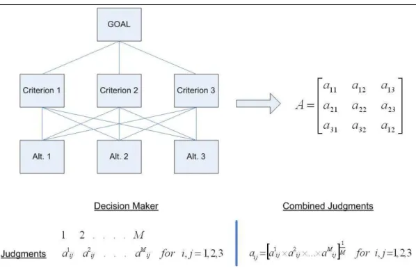
Higher complexity and need for different specializations necessitate the partic-ipation of many individuals in the decision making process. AHP allows each decision maker to specify a value and then combine the individual judgments as follows: Use the geometric mean of the individual judgments to obtain the group judgment for each pairwise comparison (see Figure 2.1). Aczel and Saaty [1] showed that the geometric mean is the uniquely appropriate rule for combin-ing judgments in the AHP because it preserves the reciprocal property in the combined pairwise comparison matrix.
In Figure 2.1, a simple hierarchy is given, and matrix A which may be formed by the evaluation of criterions or evaluation of alternatives with respect to a criteria is shown. M is the number of decision makers and each of them evaluate pairwise comparisons individually, so, for the same set of pairwise comparisons, there are M different A matrices. The combined judgments are obtained as shown in Figure 2.1, by taking geometric mean of each element of A matrices.
M different A matrices are transformed to one A matrix which is formed by
2.2.5
Deriving Relative Weights
The next step is to estimate the relative weights of the decision elements by using the eigenvalue method. The mathematical basis for determining the weights has been determined by Saaty [13] based on matrix theory. The procedure is called an eigenvector approach, which takes advantage of characteristics of a special type of matrix called a reciprocal matrix.
The entries aij are defined by equation 2.2 and according to 2.3 the consistent
pairwise comparison matrix, A in 2.1, can be represented in the form shown in 2.4 A = w1 w1 w1 w2 w1 w3 . . w1 wn w2 w1 w2 w2 w2 w3 . . w2 wn w3 w1 w3 w2 w3 w3 . . w3 wn . . . . wn w1 wn w2 wn w3 . . wn wn (2.4)
The objective is to find eigenvector w corresponding to maximum eigenvalue
λmax which is the relative weights of the objects:
w = (w1, w2, w3, ..., wn) (2.5)
If the pairwise comparison matrix is not consistent as stated above, the weights of the objects obtained by using eigenvalue method may not be valid. For this reason we should check the consistency of the matrix A.
2.2.6
Checking Consistency of the Results
In decision-making, it is important to know how good the consistency is. Con-sistency in this case means that the decision procedure is producing coherent judgments in specifying the pairwise comparison of the criteria or alternatives.
The cardinal consistency rule is:
aijajk = aik for i, j, k = 1, ...n. (2.6)
When A is consistent, and
aij = wi wj ⇒ wi = aijwj for i, j = 1, ....n. (2.7) Aw = a11 a12 . . . a1n a21 a22 . . . a2n . . . an1 an2 . . . ann w1 w2 . . . wn = w1 w1 w1 w2 w1 w3 . . w1 wn w2 w1 w2 w2 w2 w3 . . w2 wn w3 w1 w3 w2 w3 w3 . . w3 wn . . . . wn w1 wn w2 wn w3 . . wn wn w1 w2 . . . wn Aw = w1+ w1+ ... + w1 w2+ w2+ ... + w2 . . . wn+ wn+ ... + wn = nw1 nw2 . . . nwn Aw = nw (2.8)
In matrix theory, equation (2.8) is satisfied only if w is an eigenvector of A with eigenvalue of n.
All the rows in the represented matrix are constant multiplies of the first row. From linear algebra all the eigenvalues λi, i=1,...n are zero except one. Since A
is a reciprocal matrix and all the entries are positive, all the eigenvalues of A are non-negative. Therefore λi which is greater than zero can be called λmax.
n X i=1
Table 2.2: Random Indices (RI)[13]
n 1 2 3 4 5 6 7 8 9 10 11 12 13 14 15 RI 0 0 0.52 0.89 1.11 1.25 1.35 1.4 1.45 1.49 1.51 1.48 1.56 1.57 1.59
The trace of a matrix is a summation of the diagonal entries. Since all the diagonal elements of A are one, the trace of A is n.
Since all the eigenvalues λi are zero except λmax, n
X i=1
λi = λmax (2.10)
This implies that λmax = n and λmax can be used as an approximation for n.
An index is needed to measure the consistency of weights. The following index, the consistency index (CI ), was suggested by Saaty [13]:
Consistency Index, CI = λmax− n
n − 1 (2.11)
This is an index to assess how much the consistency of pairwise comparisons differs from the perfect consistency. The numerator signifies the deviation of maximum eigenvalue (λmax) from perfect consistency, which is n. The
denomina-tor is needed to compute an average of each pairwise comparison from perfectly consistent judgment. A value of one subtracted from the order of matrix n, be-cause one of the pairwise comparisons is a self-comparison, and there should be no inconsistency involved in self-comparison.
The consistency check of pairwise comparison is done by comparing the com-puted consistency index with the average consistency index of randomly generated reciprocal matrices using one-to-nine scale . Table 2.2 shows the random indices (RI) for matrices of order 1 through 15. RI values are taken from Saaty [13].
AHP measures the overall consistency of judgments by means of a consis-tency ratio (CR). The consisconsis-tency ratio is obtained by dividing the computed consistency index by the random index.
CR = CI
Saaty [13] stated that a consistency ratio of 0.10 or less can be considered acceptable; otherwise the judgments should be improved.
2.2.7
Synthesis of Priorities
After finding normalized eigenvectors (sum up to 1) that corresponds to λmax’s
for each evaluation, and verifying that the pairwise comparisons are acceptable in terms of consistency criteria, the last step is the synthesis of priorities. Priorities are synthesized from the top level down by multiplying local priorities by the priority of their corresponding criterion in the level above, and adding them for each element in a level according to the criteria it affects. (The second level elements are each multiplied by unity, the weight of the single top level goal.) This gives the composite or global priority of that element which is then used to weigh the local priorities of elements in the level below compared by it as criterion, and so on to the bottom level. [13]
2.2.8
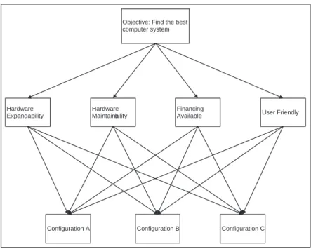
A Numerical Example
To clarify AHP methodology, it is appropriate to investigate a numerical example. We take an example from Triantaphyllou and Mann’s [20] work. Suppose that the best computer system is tried to be chosen among three alternative configurations (configuration A, configuration B, configuration C). We have four criteria which are ‘hardware expandability’, ‘hardware maintainability’, ‘financing available’, and ‘user friendly’. The hierarchical structure can be seen from Figure 2.2. For this hierarchical structure, the evaluation process has five main parts:
1. Evaluation of criteria with respect to the objective
2. Evaluation of alternative configurations with respect to criterion ‘hardware expandability’
3. Evaluation of alternative configurations with respect to criterion ‘hardware maintainability’
4. Evaluation of alternative configurations with respect to criterion ‘financing available’
5. Evaluation of alternative configurations with respect to criterion ‘user friendly’
In case there is only one decision-maker, for each evaluation part we form an A ma-trix as in Figure 2.3. For each A mama-trix we estimate the relative weights/priorities by using the eigenvalue method, and then we check the consistency. In Figures 2.4, 2.5, 2.6, 2.7 you can see A matrices for other evaluation parts with priority vectors and consistency ratios (CR). The priority vectors are used to form the en-tries of the decision matrix. The decision matrix and the resulted final priorities are in Figure 2.8. The final priority for each alternative configuration is obtained by multiplying the columns of the decision matrix (each column corresponds to a criterion) with the corresponding criterion’s weight, then by taking summation of the elements for each row (each row corresponds to an alternative), and finally, by normalizing the resulting vector such that summation of the vector is equal to one.
Figure 2.2: Hierarchical Structure of Numerical Example
Objective: Find the best computer system Hardware Expandability Hardware Maintainability Financing
Available User Friendly
Configuration A Configuration B Configuration C
Figure 2.3: A Matrix for Criterion ‘Hardware Expandability’
Figure 2.5: A Matrix and Priority Vector for Criterion ‘Hardware Maintainability’
Figure 2.6: A Matrix and Priority Vector for Criterion ‘Financing Available’
2.2.9
Criticisms of AHP and a Variant of AHP
The AHP and its use of pairwise comparisons has inspired the creation of many other decision-making methods. Beside, its wide acceptance, it also created some considerable criticism. Belton and Gear(1983) [2] observed that the AHP may reverse the ranking of the alternatives when an alternative identical to one of the already existing alternatives is introduced (well-known rank reversal problem). In order to overcome this deficiency, Belton and Gear proposed that each column of the AHP decision matrix to be divided by the maximum entry of that column. Thus, they introduced a variant of the original AHP, called the revised-AHP. Later, Saaty [16] accepted the previous variant of the AHP and now it is called the Ideal Mode AHP. The following guidelines were developed by Millet and Saaty [10] to reflect the core differences in translating performance measures to preference measures of alternatives. The original AHP should be used when the decision maker is concerned with the extent to which each alternative dominates all other alternatives under the criterion. The Ideal Mode AHP should be used when the decision maker is concerned with how well each alternative performs relative to a fixed benchmark. For example, consider selecting a car:
Two different decision makers may approach the same problem from two dif-ferent points of view even if the criteria and standards are the same. The one who is interested in “getting a well performing car” should use the Ideal Mode. The one who is interested in “getting a car that stands out” among the alternatives should use the original AHP. [17]
Another main drawback of AHP, is the high number of pairwise comparisons, especially for large hierarchies. Assigning a numerical value for each pairwise comparison is also not easy. For this reason, for large number of pairwise com-parisons, considerable amount of effort is needed.
2.3
Multicriteria Clustering
Projects are evaluated in terms of features by using a multicriteria decision mak-ing methodology, AHP. The next step is the clustermak-ing of projects.
The two mostly used technique for grouping objects with similar properties are: classification and clustering. Generally both names are used interchangeably but some important differences exist between them. Classification techniques use supervised learning; which means that the objects are assigned to pre-defined classes. On the contrary, clustering is an unsupervised technique that finds po-tential groups in data such that the objects within a cluster are more similar to each other than to objects in other clusters [19].
In literature, the research related to grouping objects with respect to multiple criteria are mainly focused on the assignment of actions to pre-defined classes; in other words multicriteria classification field [19]. Since the model studied in this thesis requires a multicriteria clustering method, only clustering part of the field is given.
In the context of AHP, so far we have found three different applications in literature, related to multicriteria clustering field. Two of them can be considered as extensions of AHP method. The third one is a kind of generic method that can be applied by using the results of any multicriteria decision methodology.
2.3.1
AHP Based Clustering
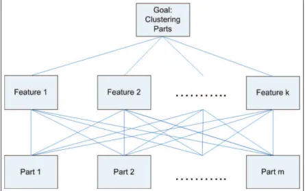
Ben-Arieh and Triantaphyllou [3] used the AHP in the group technology appli-cation. The problem discussed in the paper is grouping N different part types based on a predetermined set of features. In the proposed methodology, parts’ data about different features are expressed in terms of membership values. That is, for each part, the membership value of a given feature in the part is determined. The hierarchy of the model can be seen at Figure 2.9. As it can be seen from
the hierarchy, the features are considered as criteria, and the parts are considered as the alternatives. Membership values are the weights of the parts for each feature. In this work, the method used for determining membership values is based on Ideal Mode AHP.
Three types of features are identified in the paper:
1. Quantitative features. Such features represent properties of parts that can be expressed numerically.
2. Qualitative(fuzzy) features. These features describe the part attributes in fuzzy terms such as ‘large, medium, small’ or other terms agreed upon by the system users.
3. Quantitative features with subjective meaning. Features of this type have numerical values which do not quantitatively represent the actual meaning of these features in the relevant environment. Therefore these features are also fuzzy.
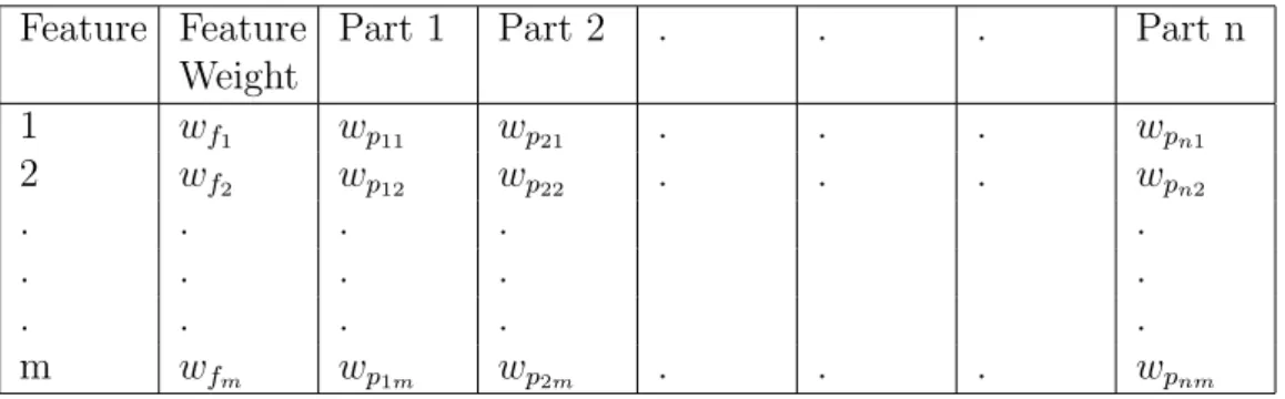
The method presented in the paper treat the fuzzy features and quantitative features differently. For the fuzzy features, the membership values are determined by using Ideal Mode AHP. The membership values for the quantitative features are determined by normalizing the values such that the maximum one is equal to one. The membership matrix can be seen in Table 2.3 where wfk represents the weight of Feature k (where k = 1....m), and wpsr represents the membership value of Feature r (where r = 1....m) in the Part s (where s = 1....n).
According to Ben-Arieh and Triantaphyllou [3], once the features that are used for the part grouping are described in terms of their membership values, and their relative importance, it is possible to cluster the parts into groups. Two different ways are proposed to conduct grouping process:
1. Matrix-based clustering: By multiplying the membership values of the fea-tures by the feafea-tures’ weight (importance), a new matrix is generated. In this matrix, each part is represented as an m dimensional point in Euclidean
Table 2.3: Membership Table Feature Feature
Weight
Part 1 Part 2 . . . Part n
1 wf1 wp11 wp21 . . . wpn1 2 wf2 wp12 wp22 . . . wpn2 . . . . . . . . . . . . . . . m wfm wp1m wp2m . . . wpnm
space(each feature is a different dimension). Using this matrix, grouping is accomplished by using any clustering method.
2. Aggregate-value clustering: Each part represented by an aggregate value which is vi = m X j=1 wfjwpij for i = 1, ....n. (2.13) Then parts are clustered based on these single values.
2.3.2
VAHP Based Clustering
Zahir [25] has developed a Euclidean version of the AHP in a vector space (VAHP). Due to the fact that AHP uses summation normalization, using such nu-merical data in a subsequent clustering procedure that uses Euclidean distance as the similarity measure may be problematic. However, the VAHP based approach allows obtaining representations of objects that satisfy Euclidean normalization and thus is consistent with the use of Euclidean distance in the clustering tech-nique. [26]
The VAHP has the same decision hierarchy as the conventional AHP and uses the same eigenvector method. The decision space is assumed to be a linear vector space spanned by the number of objects to decide from and each eigenvector is defined with an Euclidean norm. However, here Zahir [25] introduces the preference operator P obtained by taking the square roots of each element of A, where A is the corresponding preference matrix of the conventional AHP. If A is consistent, P is also consistent and λmax = n for both. If the eigenvector w of
A, such that Pwi = 1, the eigenvector v of P is normalized such that vTv = 1
orPni=1 v2
i = 1. According to ‘Eigenvalue Power Law’ theorem [15] only when A
satisfies the generalized consistency condition, we have vi =
√
wi or wi = vi2. This
preserves the validation successes of conventional AHP. Thus, as we interpret wi
as the relative priority for A, v2
i is taken as the relative priority for P .
To sum up, the VAHP uses the same structure, the same decision hierarchy, the same eigenvector method, and it makes it possible to develop a meaningful grouping or clustering technique based on Euclidean distance.
2.3.3
An extension of the k-means algorithm
Smet and Guzman [19] proposed an extension of the well-known k-means algo-rithm to the multicriteria framework. This extension relies on the definition of a multicriteria distance based on the preference structure defined by the decision
maker. With the proposed multicriteria distance two alternatives will be simi-lar if they are preferred, indifferent, and incomparable to more or less the same actions.
The method proposed by Smet and Guzman [19] can be applied by using the results of any multicriteria decision making method. It just needs the preference structure as the input to partition the set of alternatives into classes that are meaningful from the multicriteria perspective.
2.3.4
General Clustering Algorithms
2.3.4.1 K-Means Clustering Algorithm
The k-means clustering algorithm is one of the simplest and the most commonly used algorithms. It employs squared error similarity criteria, which is widely used criterion function in clustering. It starts with predefined number (k) of initial set of clusters and at each iteration, patterns/objects, that are tried to be clustered, are reassigned to the nearest cluster based on the distance based similarity measure, this process is repeated until a converge criterion is met such as no reassignment of any pattern to a new cluster or predefined error value. [9]
In detail, the algorithm of the method is as follows:
There are n input patterns and patterns are denoted by P1, P2, ., Pn. The
pattern Pi (ith pattern) consists of a tuple of describing features where features
are denoted by fi1, fi2, . , fid. A dimension represents each feature, where d is
the number of dimensions of the value space. The second input of the algorithm is the predefined number of clusters, denoted by k. The number of the clusters cannot be changed during the execution of the algorithm. Let C1, C2,., Ck be the
clusters, and each cluster is represented by its centroid. Let c1, c2, . , ck be the
centroids of the clusters.
First, the initial cluster centroids are formed randomly. The distances between pattern Pi and all clusters are calculated and pattern Pi is assigned to the closest
cluster Cd. This process is repeated for all patterns and all patterns are assigned
to a unique cluster. At the end of the iteration all centroids (c1,c2, . , ck)
are updated. In the next iteration, distance calculations between patterns and clusters are repeated with the updated centroids. The algorithm will iterate until predefined number of iteration is reached or no pattern is moved to a different cluster. At the end of the algorithm, quality of the clustering is measured by the error function: E = k X d=1 X Pi∈Cd kPi− Cdk2 (2.14)
Moreover, we need a measure of how good the clusters, so that we can choose the right value of k. The silhouette value for each object is a measure of how similar that object is to objects in its own cluster compared to objects in other clusters, and ranges from -1 to +1. It is defined as
s(Pi) =
b(Pi) − a(Pi)
max(a(Pi), b(Pi)) (2.15)
where
a(Pi) = average dissimilarity of Pi to all other objects of A d(Pi, C) = average dissimilarity of Pi to all objects of C
b(Pi) = min
C6=Ad(Pi, C)
where A is the first assigned cluster of object Pi, and C is any cluster different
from A. As the s(Pi) value comes close to 1, it means that object i is at the right
cluster. The average of the s(Pi) for i = 1, 2, ..., n which is called the average
silhouette width for the entire data set can be used for the selection of a ‘best’ value of k, by choosing that k for which the average silhouette width for the entire data set is as high as possible. [9]
The objective of the k-means clustering algorithm is to select the best clus-tering with k groups.
2.3.4.2 Hierarchical Clustering Algorithm
Hierarchical algorithms do not construct a single partition with k clusters, but they deal with all values of k in the same run. That is, both the partition with
k = 1 and the partition with k = n are part of the output. The output is in the
form of dendrogram, where nested partitions and similarity levels at partitions change are presented. [9]
There are two basic approaches in hierarchical clustering:
• Agglomerative (starts when all objects are apart, the case where there are
n clusters, and merges two clusters at each step until only one is left.)
• Divisive (starts with when all objects are together, the case where there is
one cluster, and splits up clusters at each step, until there are n clusters.)
Due to its advantages and easy to implement speciality, agglomerative hier-archical clustering algorithms are used frequently. It starts when all objects are apart and in all succeeding steps, the two closest clusters are merged.
Hierarchical methods suffer from the defect that they can never repair what was done in previous steps. Indeed, once an agglomerative algorithm has joined two objects, they can not be separated anymore. Also, a cluster that has been split up by a divisive algorithm can not be reunited. [9]
The objective of hierarchical clustering algorithms is not finding the best clusterings but to describe the objects in a totally different way.
Model and The Analysis
Based on the studies related to project management in literature, we observed that “a project is a project” is the dominating idea. However the idea that dif-ferent projects must be managed in difdif-ferent ways, comes out from the real-life applications at MST, one of the three divisions of Aselsan, as a need. What we need is basically a framework to distinguish projects that have common char-acteristics that are meaningful in terms of project management concept. Then practical guidelines on how to manage projects in different ways can be estab-lished. However creating such a framework which has substantial importance for the company, Aselsan, requires great effort.
Our strategy for creating the framework can be summarized as follows:
1. Firstly, we look at the clustering of projects for which data is available. The natural groupings among the projects hopefully come out.
(a) The features that can reveal the differences between the projects in terms of project management concept are determined.
(b) The projects for which data is available, and there is no problem to be evaluated for the clustering work are determined.
(c) After obtaining the related data of the projects, projects are clustered by using appropriate methods.
2. Secondly, the project groupings are examined to see whether they are mean-ingful and they can be used for creating the framework.
3. By benefiting the proposed frameworks in the literature and the project groupings that come out in previous steps, the framework is created.
In this thesis we focused on (1c), “After obtaining the related data of the projects, projects are clustered by using appropriate methods.”
The problem discussed in this study is grouping N different projects based on a predetermined set of features. It is a multicriteria clustering problem. Basically, the problem has two parts:
Defining the projects in terms of features: The amount of each of the fea-tures that each project possesses is measured by using a multicriteria deci-sion method. In other words, if we think each feature as a fuzzy set, we are trying to find membership values of projects for each fuzzy set.
Clustering the projects: The projects are clustered based on the representing vectors that are formed with the amount of each of the features that each project possesses.
3.1
Defining The Projects In Terms of Features
The choice of method for defining the projects in terms of features, closely related with the features characteristics. For this reason, we first look at the features.
3.1.1
Features
3.1.1.1 Technological Uncertainty
In general, technological uncertainty is associated with the degree of using new (to the company) versus mature technology within the product or process. Since most projects employ a mixture of technologies, our interpretation is based on the share of new technology within the product. In addition; as a project progresses, the related technological uncertainty of project tends to change; therefore, tech-nological uncertainty of a project implies the related uncertainty at the time of project initiation.
3.1.1.2 Platform Type
Platform type defines the working environment of product(s). Platform types can be grouped under two main titles. One of them is commercial platforms, and the other one is military platforms. In general form, platform types are:
• Commercial Platforms
– Stationary Ground
– Mobile Wheel Drive Ground – Airborne
– Naval
• Military Platforms
– Stationary Ground
– Mobile Wheel Drive Ground – Mobile Tracked Ground – Airborne
– Naval
Platform types are directly related with the standards and specifications that must be obeyed. Therefore it is a crucial parameter for a project.
3.1.1.3 Work and Test Environment
Efficiency is strongly dependent on the work and test environment. Due to struc-tural and operational characteristics of systems, the work and test environment has to be sometimes a military area in battlefield conditions, sometimes a con-struction facility which does not belong to Aselsan for a considerable time in-terval. For this reason, work and test environment is the feature that should be incorporated into the evaluation of projects.
3.1.1.4 System Scope
Products are composed of components and systems of subsystems. Every product has its own hierarchy with different design and managerial implications. Projects can be classified as follows in terms of their hierarchies in its most general form :
1. Assembly project: dealing with either a single component or with a com-plete assembly (collection of components and modules combined into a sin-gle unit).
2. System project: a collection of interactive elements functioning together within a single product.
3. Array project: dispersed collection of systems that function together to achieve a common purpose.
3.1.1.5 Amount of Resource (Labor)
Human resources are extremely important for an organization like MST where tens of R&D projects are carried out concurrently. In addition, the amount of human resources (man*hour) needed for a project is an appropriate indicator about the size of the project.
We can classify the features by using the Ben-Arieh and Triantaphyllou’s [3] classification.
• Quantitative features:
– Amount of resource (labor): The numerical data of amount of resource (labor) is available for all projects.
• Qualitative fuzzy features:
– Technological Uncertainty: There is no numerical data related to tech-nological uncertainty of projects. Techtech-nological uncertainty of the projects are described by the terms low, medium, high, super high. – Platform Type: There is no numerical data related to platform types
of projects. Although each of the projects’ platform type is known, its effects to project management should be quantified.
– Work and Test Environment: There is no numerical data related to work and test environment of projects.
– System Scope: There is no numerical data related to system scope of projects. The general classification of projects as assembly, system and array is known.
As it can be seen above, four features out of five are characterized as ‘quali-tative fuzzy feature’. These features can be considered as subjective feature, be-cause for these features, projects’ related attributes may be evaluated differently by different experts. The other one, amount of resource (labor), is character-ized as ‘quantitative feature’ or objective feature. For this reason, the choice of method for defining the projects in terms of features should permit the evaluation of both objective features and subjective features.
One of the most appropriate method to quantify subjective features is using expert knowledge, so the method should aim to get expert knowledge as good as possible. Moreover, the method should permit a group of people to realize the evaluation together and/or one by one, since subjective evaluations may change from person to person and the best way to reach more accurate results is to get data from a group of people who are experts in the related area.
To sum up, we need a multicriteria decision making method, which supports subjective and objective evaluations, gets expert knowledge in an effective way, to determine the membership value of each feature in the projects. For this reason, Analytic Hierarchy Process is chosen since it is a powerful multicriteria decision making method which meets the requirements of the problem.
3.1.2
AHP Model
The model is constructed in the way that AHP methodology proposes. For this reason, the model is explained based on AHP methodology:
Overall goal (objective): The objective is to evaluate the projects in terms of project management concept.
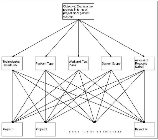
Hierarchical structure: Hierarchical structure can be seen in Figure 3.1. The hierarchy starts with the objective at the top level. The second level is formed by the features determined previously. The third level, which is the final one, is formed by the projects.
Pairwise comparisons: The elements in a level of the hierarchy are compared in relative terms with respect to a given criterion that occupies the level immediately above the elements being compared. In this model, we can distinguish two main groups of pairwise comparisons. One group is the features’ pairwise comparisons with respect to objective. The other group consists of pairwise comparisons of projects with respect to each feature. For the features’ pairwise comparisons, the question that is tried to answer for each comparison is like “Which one of the Feature A and Feature B is more important/effective than the other one with respect to project man-agement concept and how much relatively?”. For projects’ comparisons, the questions should be identified for each feature:
• For Technological Uncertainty: Which one of the Project A and
Project B has a higher degree of technological uncertainty and by how much relatively?
• For Platform Type: Which one of the Project A’s platform type and
Project B’s platform type has a stronger effect in the way to complicate the management activities and by how much relatively?
• For Work and Test Environment: Which one of the Project A’s work
and test environment and Project B’s work and test environment has a stronger effect in the way to complicate the management activities and by how much relatively?
• For System Scope: Which one of the Project A’s system scope and
Project B’s system scope has a stronger effect in the way to complicate the management activities and by how much relatively?
• For Amount of Resource (Labor): Which one of the Project A’s
amount of resource (labor) and Project B’s amount of resource (la-bor) is larger and how much relatively?
Estimation of Weights: Weights of the elements are estimated by using the eigenvalue method. Consistency of judgments is checked.
The AHP model that is described above has to conform to axioms of AHP. Below, the model is checked whether it conforms to the axioms or not.
• Axiom 1 (Reciprocal Comparison): Since the questions used to elicit the
judgments or paired comparisons are clearly, correctly stated and asking for a reciprocal relation. This axiom is conformed.
• Axiom 2 (Homogeneity): The elements of the model that are evaluated with
pairwise comparisons are comparable and they do not differ by too much in the property being compared. Both features’ set and projects’ set are homogeneous. The model conforms to Axiom 2.
• Axiom 3 (Independence): In expressing preferences, the features’
impor-tance are independent of the properties of projects. Features are evaluated with respect to their importance/effectiveness to project management ac-tivities in general, and the model conforms Axiom 3.
Figure 3.1: Hierarchical Structure
• Axiom 4 (Expectations): For the purpose of evaluating projects in terms
of project management activities, the hierarchy is assumed to be complete. Axiom 4 is conformed.
In literature, as it is mentioned, there are two versions of AHP. One of them is the original AHP which is called “Distributive Mode” and the other one is called “Ideal Mode”. By following the guidelines developed by Saaty and Millet [10], the one, which fits best to the case, must be chosen. The guideline states that the original AHP, Distributive Mode AHP, should be used when the decision
Table 3.1: Output Table
Feature Feature Weight
Project 1 Project 2 . . Project m 1- Technological
Un-certainty
wf1 wp11 wp21 . . wpm1
2- Platform Type wf2 wp12 wp22 . . wpm2 3- Work and Test
En-vironment wf3 wp13 wp23 wpm3 4- System Scope wf4 wp14 wp24 wpm4 5- Amount of Resource (Labor) wf5 wp15 wp25 . . wpm5
maker is concerned with the extent to which each alternative dominates all other alternatives under the criterion. On the other hand, Ideal Mode AHP should be used when the decision maker is concerned with how well each alternative performs relative to a fixed benchmark. In our case, main objective is to construct a general framework for projects, so the aim here is not to find the dominating project. The aim is to define projects in terms of features, and to evaluate projects relative to a fixed benchmark. For this reason, Ideal Mode AHP seems to fit best to the needs of the problem.
The output of the model explained above constitutes the features weights, and weights/membership values of projects in terms of each one of the features. In a table format, the output is like Table 3.1, where wfa defines the weight of feature numbered ‘a’, wpab defines the weight of project numbered ‘b’ with respect to the feature numbered ’a’ for a = 1, 2....5 and b = 1, 2...m.
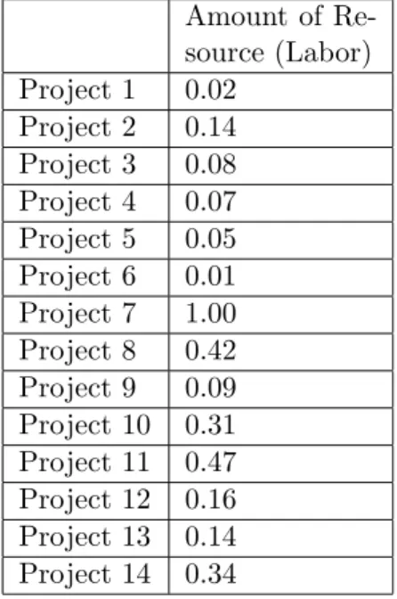
Ben-Arieh and Triantaphyllou [3] proposed a different way to evaluate alter-natives with respect to objective features. Since quantitative data is available for objective features, the alternatives do not need to be evaluated with pairwise com-parisons. By just normalizing the quantitative data such that the largest number in the vector is equal to one, the membership values of projects in terms of an objective feature are obtained. Therefore, smaller number of pairwise compar-isons have to be evaluated and experts can focus on the evaluations where expert
knowledge is the inevitable source. In our model, amount of resource (labor) is the only objective feature, and it is appropriate to obtain membership values of projects in terms of this feature by using the method proposed in Ben-Arieh and Triantaphyllou [3] work. In the output table 3.1, only wp15 wp25 . . . wpm5 values are obtained by normalizing the available quantitative data.
3.2
Clustering The Projects
Once the projects are defined in terms of features, and the features’ weights are determined, it is possible to cluster the projects into groups. However, due to the multicriteria nature of the problem, there are different views related to distance concept.
As it is mentioned, there are three applications related to multi-criteria clus-tering. The crucial differences between the applications result from different distance concepts. Ben-Arieh and Triantaphyllou [3] assumed that the matrix formed by multiplication of the features’ weights with weight/membership vec-tors of projects can be used to form representative vecvec-tors of projects. With these vectors, each project can be represented in Euclidean space where each feature is a different dimension. Hence, the distance between two projects can be calculated as the Euclidean distance of two points (representing vectors of two projects).
On the other hand, Zahir [26] states that in order to obtain a meaningful pattern discovery, the underlying similarity measure cannot be independent of the type of normalization imposed on the data. In addition, since the AHP uses summation normalization, using such numerical data in a subsequent clustering procedure that uses Euclidean distance as the similarity measure may be prob-lematic. For this reason, Zahir [25] developed a Euclidean version of the AHP in a vector space (VAHP). The VAHP based approach allows obtaining representa-tions of objects that satisfy Euclidean normalization and thus is consistent with the use of Euclidean distance in clustering technique.
In Smet and Guzman’s work [19], a multicriteria distance, based on the pref-erence structure defined by the decision maker, is proposed. This multicriteria distance is based on the idea that two alternatives will be similar if they are pre-ferred and indifferent to more or less the same features. In preference modelling, usually the following relations are considered:
aiP aj if ai is preferred to aj, aiIaj if ai is indifferent to aj, aiJaj if ai is incomparable to aj.
The multicriteria distance definition proposed by Smet and Guzman [19] is:
d(ai, aj) = 1 − P4 k=1|Pk(ai) ∩ Pk(aj)| n (3.1) where • P1(ai) = {aj ∈ A|aiJaj}, • P2(ai) = {aj ∈ A|ajP ai}, • P3(ai) = {aj ∈ A|aiIaj}, • P4(ai) = {aj ∈ A|aiP aj},
In AHP, since there is no incomparable relation, the J relation remains empty and the comparison between pairs of actions are restricted to P and I relations. In this thesis, all the distance concepts mentioned above are applied in project clustering application by using well-known clustering algorithms: k-means and hierarchical clustering.
Application of Project Clustering
In this section, we present the details of the application performed in Aselsan. We look at the clustering of projects, and we expect that the natural groupings among the projects come out. Based on the model, the projects are evaluated with respect to predefined features by using AHP, and the representing vectors are formed for each project. Then, by using well-known clustering algorithms, k-means and hierarchical clustering, the projects are clustered.
For this study, fourteen projects are chosen to be evaluated. The set of four-teen projects is assumed to represent the full set of MST’s applications. Since Aselsan is in military electronic sector, and most of its projects have high se-crecy, we can not give the names of the projects in this study. However, we will mention the characteristics of the projects while the project clusters are being investigated.
Experts, as being the main source of projects’ data, are the most important actors of the model. The projects are evaluated by experts with respect to all features except ‘Amount of Resource (Labor)’ feature which was identified as objective feature in the model. Moreover, project clusters coming out of the model are investigated by the experts to see whether they are meaningful or not. For this reason, two issues gain importance:
• Selection of experts
• Common understanding of the concepts used in the model
The vital characteristic for experts is to have enough knowledge about the set of fourteen projects such that for each subjective feature, pairwise comparisons of projects can be realized consciously. Since some of the projects out of the set of fourteen projects started at the beginning of 1990s, the number of possible experts possessing the vital characteristic is small. Among the possible candidates, four managers of MST kindly accept to provide data about the projects and to be part of the study.
Lack of common understanding of the concepts causes high group inconsis-tency and getting low quality of data which harms the quality of output, project clusters. For this reason, before initializing the process, we have worked together with the experts to give a common meaning to each concept in the model. The projects have also been discussed.
Expert Choice is the most well-known AHP software. In fact, Expert Choice is a software which has accelerated the wide-spread use of AHP. However, Expert Choice software is unavailable at Aselsan and the trial version of it restricts the number of alternatives to eight. For this reason, we create a software called ‘ProTer ’. ProTer is a stand-alone AHP software that is capable of group decision making. The model’s AHP part is conducted by using ProTer (Figure 4.1). You can find more information related to ProTer in Appendix.
4.1
Application of AHP
In application of AHP, there are two main parts:
• Evaluation of Features
• Evaluation of Projects
All four experts perform both evaluation of features and evaluation of projects.
4.1.1
Evaluation of Features
In this part of the study, all the features including both the subjective features
• Technological Uncertainty • Platform Type
• Work and Test Environment
• System Scope,
and the objective feature
• Amount of Resource (Labor)
are evaluated with pairwise comparisons by the experts. Since there are 5 features, each expert evaluate 10 pairwise comparisons. (Number of Pairwise Comparisons
= n×(n−1)2 , where n is the number of elements being evaluated.) You can find
input values in Appendix.
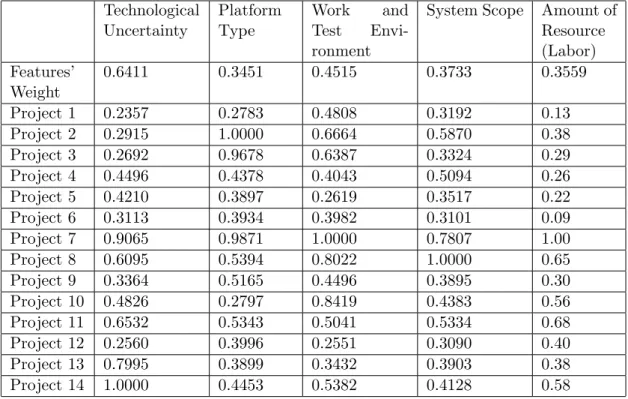
After all the pairwise comparisons are evaluated by all the experts, the weights of the features can be calculated by using the AHP methodology. The results are as in Table 4.1.
Table 4.1: Features’ Weights
Feature Weight of the Feature Technological Uncertainty 0.41
Platform Type 0.12 Work and Test Environment 0.20 System Scope 0.14 Amount of Resource(Labor) 0.13
As it can be seen from Table 4.1, ‘Technological Uncertainty’ feature is the dominant feature such that its weight nearly equals to two times of the weight of the second important feature of all, ‘Work and Test Environment’.
The final weights of features are approved by the experts.
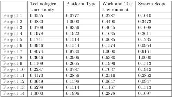
4.1.2
Evaluation of Projects
In this part of the study, all fourteen projects are evaluated pairwise by the experts in terms of the subjective features. For the objective feature, since we have the quantitative data, there is no need for the projects to be evaluated with pairwise comparisons.
Each expert, for each of the feature (subjective ones), has to evaluate 91 (Number of Pairwise Comparisons = 14×(14−1)2 ) pairwise comparisons which is quite a high number. Totally, experts evaluated 364 (91×4) pairwise comparisons. (You can find input values in Appendix.) High number of pairwise comparisons is one of the weak points of AHP.
After all the pairwise comparisons are evaluated by all experts, the weights of the projects for each subjective feature can be calculated by using the eigenvalue method. The results are as in Table 4.2.
As it is seen at Table 4.2, for each feature, the weight vectors are normalized such that the max value is equal to one. This type of normalization is the result