A comparative study of computational procedures for resource constrained project scheduling problem

A COMPARATIVE STUDY OF COMPUTATiONAL

PROCEDURES FOR RESOURCE CONSTRAIMED

PROJECT SCHEDULING PROBLEM

A TH E SiS

TO TK£

Or Ji^DUSTHiAL

AND THE !MSnTiJTS

OF

ii^SU^SSRITJS

SOiEiiOfS

OF

B!LK£3

^T Ui^r/iiiSJTY

m

PARTS AL fULP2l,L?tiiiS£irf O r THE aiOU=)?32?A«:-iTS

FOR THE 0 2 0 H E S o ?

M4TTSR Dr SCiiHDE

A COMPARATIVE STUDY OF COMPUTATIONAL

PROCEDURES FOR RESOURCE CONSTRAINED

PROJECT SCHEDULING PROBLEM

A T H E SIS S U B M IT T E D T O T H E D E P A R T M E N T O F IN D U S T R IA L E N G IN E E R IN G A N D T H E IN S T IT U T E O F E N G IN E E R IN G A N D SC IE N C E S O F B IL K E N T U N IV E R S IT Y IN P A R T IA L F U L F IL L M E N T O F T H E R E Q U IR E M E N T S F O R T H E D E G R E E OF M A S T E R O F SC IE N C E

By

' í ¿ ’ 5 '

' з з /

0 Copyright July, 1991 by

I certify tliat I have read this thesis and that in my opinion it is fully adequate, in scope and in quality, as a thesis for the degree of Master of Science.

Associate. Prof. Dr. Osi^an Oğuz (Principal Advisor)

I certify that I have read this thesis and that in my opinion it is fully adequate, in scope and in quality, as a thesis for the degree of Master of Science.

Prof. Dr.« Akif Eyler

I certify that I have read this thesis and that in my opinion it is fuUy adequate, in scope and in quality, as a thesis for the degree of Master of Science.

Associate P i^ .’ Dr. Cemal Dinçer

Approved for the Institute of Engineering and Sciences:

Prof. Mehmet Batay

Director of Institute o f Engineering and Sciences

ABSTRACT

Supervisor: Associate. Prof. Dr. Osman Oğuz July, 1991

Customarily, the project sclieduling problem is thought in the context of PER T and CPM. Although widely used and powerful, these techniques do not take into account a basic feature of the problem, that is resource limitations. The problem addressed in this study is to schedule the activities of a single project in order that all resource and precedence relationships constraints are satisfied with an objective of minimizing total of activity completion times. Our purpose is to make a computational comparison of some solution procedures for the problem. Firstly, the 0 - 1 formulation of the problem is introduced together wdth the underlying assumptions. Then, we describe the solution procedures tested in this study. In order to evaluate them, the random activity networks are generated. Finadly, we provide the results and conclusions.

K e y w o r d s : Project Management, Scheduling, Heun^vics.

ÖZET

K A Y N A K KISITLI PROJE ÇİZELGELEM E PR O B LE M İ ÇÖZÜM TEKN İKLERİN İN

K ARŞILA ŞTIRM ALI AN A LİZİ

Haşan Bala

Endüstri Mühendisliği Bölümü Yüksek Lisans Tez Yöneticisi: Doç. Osman Oğuz

Temmuz, 1991

Ahşıla geldiği üzere, proje çizelgeleme problemi P ER T ve CPM bağlamında düşünülür. Bu teknikler çok etkili ve yaygın olarak kuUanılmalarına rağmen, söz konusu problemin temel bir özelliği olan kaynak kısıtlayıcılarını gozardı ederler. Bu çalışmada incelenen problem, bir projenin faaliyetlerini tüm kaynak ve on ilişkiler kısıtlayıcıla­ rını sağlayacak ve faaliyet bitiş zamanlarının toplamını enazlayacak şekilde çizelgelemektir. Çalışmanın amacı, sözkonusu problem için bazı çözüm tekniklerinin karşılaştmıalı analizini yapmaktır, ilk olarak, problem, yapılan varsayımlarla birlikte 0-1 tamsayı programlama tekniği ile formüle edilmiştir. Daha sonra, sözü edilen çözüm teknikleri tanıtılmıştır. Bu teknikleri değerlendirebilmek amacıyla rastgele problemler türetilmiştir. Son olarak, sonuçlara ve değerlendirmelere yer verilmiştir.

To my parents,

ACKNOWLEDGMENT

I would like to thank Assoc. Prof. Osman Oğuz for his supervision, guidance, suggestions, and encouragement throughout the development of this thesis. I am indepted to him for the help o f providing the program of MIXED heuristic. I am grateful to Prof. Akif Eyler, and Assoc. Prof. Cemal Dinçer for their valuable comments.

I would like to extend my deepest gratitude and thanks to my parents for their morale support, encouragement, especially at times of despair and hardship.

I would like to offer my sincere thanks to my friends who provided morale support and en- courgement. I wish to express my appreciation to Nazan Titrek, Gündüz Cöner and all other BCC personel for their help.

Contents

1 IN T R O D U C T IO N

2 L IT E R A T U R E R E V IE W

2.1 Time-Cost Trade Off Techniques... 3

2.2 Resource Leveling Procedures 2.3 Resource Constrained Scheduling T e c h n iq u e s... 4

2.3.1 Heuristic Approaches... 5 2.3.2 Optimization A p p ro a c h e s... 6 3 P R O B L E M F O R M U LA TIO N A N D SOLUTION P R O C E D U R E S 3.1 Problem Formulation 3.2 Solution Procedures... 12 3.2.1 M IX E D H e u ristic... 13

3.2.2 M IN SLK , SDFIRST and LDFIRST Heuristics ... 15

3.2.3 Optimizing Software S C I C O N I C ... 17

4 E X P E R IM E N T A T IO N A N D RESULTS 20 4.1 Problem Generation... 20

4.2 Design of A nalysis... 22

CONTENTS IX

4.3 Results of the S t u d y ... 24

5 C O N C L U SIO N S A N D R E C O M M E N D A T IO N S 28

A P P E N D IX A 30

List of Figures

3.1 The Flowchart of MINSLK H euristic... ' ... 18

3.2 The Flowchart of Scheduling Routine... 19

List of Tables

4.1 The input range for parameters 22

4.2 List of diiferent combinations of rt and dm 23

A .l The size and density of the generated problems in com bination#! 31

A .2 The size and density of the generated problems in combination # 2 ... 31

A.3 The size and density of the generated problems in combination # 3 ... 32

A.4 The size and density of the generated problems in combination # 4 ... 32

A.5 The size and density of the generated problems in combination # 5 ... 33

A .6 The size and density of the generated problems in combination # 6 ... 33

A .7 The results by SCICONIC for the test problems in combination # 1 ... 34

A .8 The results by SCICONIC for the test problems in combination # 2 ... 34

A .9 The results by SCICONIC for the test problems in combination # 3 ... 35

A .10 The results by SCICONIC for the test problems in combination # 4 ... 35

A .11 The results by SCICONIC for the test problems in combination # 5 ... 36

A .12 The results by SCICONIC for the test problems in combination # 6 ... 36

A .13 The computational results by heuristics for the test problems in combination # 1 37

A .14 The computational results by heuristics for the test problems in combination # 2 37

A. 15 The computational results by heuristics for the test problems in combination # 3 38

LIST OF TABLES Xll

A. 16 The computationcLl results by heuristics for the test problems in combination ^4 38

A .17 The computational results by heuristics for the test problems in combination 39

A. 18 The computational results by heuristics for the test problems in combination #6 39

Chapter 1

INTRODUCTION

Since the development of PERT and CPM techniques in the mid 1950s, project scheduling prob­ lems have been a source of interest for researchers. The resource constrained project scheduling problem is especially important for practitioners due to the wide variety of applications such as design of production facilities, installation of computer systems, large scale construction projects, missile development, scheduhng of radio and television, maintenance projects, new product in­ troduction, etc. It is also challenging problem for mathematicians due to its computational complexity. This is maiidy because^ the general resource scheduling problem belongs to the class of NP-complete problems [16].

In CPM /PERT procedures, it is assumed that there is an infinite amount of resources avail­ able for each activity in the project network. In other words, the critical path calculations are based solely on the time requirements of the activities, regardless of the resource needs of each activity. This limiting assumptions led many researchers to investigate different techniques to incorporate resource constraints into project network analysis.

Davis [5] classified the types of procedures that have been developed into three categories:

■/. Time-cost trade off techniques

a. Resource leveling techniques Hi. Resource constrained techniques

Our study focuses on the third category. The problem addressed here is to schedule the activities of a project so that none of the resource constraints, and nor any of the j/recedence relationships

CHAPTER 1. INTRODUCTION

is violated v/ith an objective of minimizing the total completion time.

Holloway [12] provides a classification of resource constrained project scheduling problems us­ ing the number of resource types, resource availabilities and resource requirements. The specific problem in this study is the multiple constrained-resource, single project scheduling problems wdiich falls into the category of types n /n /n , according to Holloway’s [12] notation, in which n’s, in order, stand for multiple resource t}-pes, multiple units of resources, multiple number of resource types required by an activity. It is assumed that an activity can not be interrupted once begun(non-preernptive case). Further, both the resource availabilities and the resource consumption are assumed to be stationary, that is, they remain constant throughout the project duration. The 0-1 formulation of the problem, modified from Pritsker et ah [22], is given in Section 3.1.

Our intention is to give a computational comparison of heuristics for the problem addressed above. The first heuristic tested here works with a penalty function designed to solve integer programming problems. It is a general purpose Integer Programming heuristic. The second consists of three heuristics wdiich shows variation in prioritizing activities in the project. These heuristics fall into parallel approach that is to be discussed in Section 2.3.1. The third which is an optimizing software named seeks to find a near optimum solution of the reduced problem. The reduced problem is handled via a reduction process with the expense of informa­ tion loss in the objective function. In order to test the performance of these heuristics, w’e use randomly generated activity networks.

Organization of the thesis as follows : In Chapter 2, a related literature review is provided. In Chapter 3, the problem formulation and solution procedures tested are given. In Chapter 4, the experimentation and results are discussed. In Chapter 5, conclusions and recommendations are stated.

Chapter 2

LITERATURE REVIEW

Although PERT and CPM are considered to be the basis of the most successful project plan- ning/scheduling techniques, these procedures can not be used in many real life projects. This is due to the fact that these techniques were based upon the assumption that all resources con­ sumed by the project activities were available in ample quantities. Recognizing this limitation of CPM /PERT procedures, a great deal of research attention in the past three decades has been devoted to the development of scheduling techniques which take the resource constraint into consideration.

Although our study focuses on third category in the classification of Davis [5], we tliink that it is proper to supply a background about the other two categories.

2.1

Time-Cost Trade Off Techniques

Time-cost trade off procedures are based on the fact that the performance of some or all project activities can be accelerated by the allocation of more resources at the expense of higher activ­ ity direct cost. This leads to many different comidiiations of activity durations ranging from an upper normal value, associated with a normal cost, down to a lower crash value, with an associ­

ated higher cost. However, each combination may result in a different value of total project cost. So, these procedures are developed to determine the least-cost schedule for any given project duration.

Kelly and Walker [14] give examples of the basic time-cost trade off procedure. The pro­ cedure described is based on linear programming and is implemented through a network flow algorithm. It produces the minimum cost curve of project duration and detailed activity start- finish times associated w’ith every point on the curve.

CHAPTER 2. LITERATURE REVIEW 4

It is important to note that these procedures do not expbcitly take the resource limitations into account. That is they do not produce a minimum cost schedule that will satisfy the stated constraints on the availability of resources. Another point to mention about time-cost trade off procedures is that they have not been widely implemented in practice. The reasons are due to the amount and complexity of input data required for analysis.

2.2

Resource Leveling Procedures

In some project scheduling situations, resources are available in ample quantities. However, project managers may not be willing to pay the expenses involved in changing resource levels. Resource leveling techniques are useful in such cases. They provide a means of distributing resource usage over time to minimize the period-by-period variations. They can also be used to determine whether peak resource requirements can be reduced with no increase in project duration.

The underlying idea of resource leveling procedures is to reschedule the activities of a project within the limits of available slack to achieve a better distribution of resource consumption in which activity slacks are determined from CPM calculations. CPM programs with resource leveling features have been available since 1960s. Levy and Wiest [17] gives a good description of how such a program operates. However, if the available resources are tightly constrained, these procedures do not give satisfactory results. Then, the problem falls into another category of procedures which is the subject of next section.

2.3

Resource Constrained Scheduling Techniques

Since the pioneering work of Kelley [14] and Wiest [30] the resource constrained project schedul­ ing problem has occupied a great number of researchers. Over the past three decades, there have been more than 80 publications and theses that have investigated the diiTerent versions of this challenging problem. These versions can be divided into categories according to the number

CHAPTER 2. LITERATURE REVIEW

of simultaneously scheduled projects(single, multiple), the nature of the optimizing objective function, the nature of resources and the activities in the project [2].

The resource constrained project scheduling techniques can be categorized into two major groups:

i. Heuristic, or approximate procedures which are designed to produce good resource-feasible

schedules,

a. Optimization techniques to develop the best schedule.

2 .3 .1 Heui'istic Approaches

Due to the combinatorial nature and complexity of resource constrained project scheduling problem, heuristic procedures have been studied extensively. There is a vast literature on heuristic approaches. These procedures have been desig:.<‘d to solve both the scheduling of multiple projects and single projects. Early studies have appeared in 1960s. They were given by Wiest [29] and Fendly [10]. There are several attempts including comparative studies in between the e.xisting heuristics and between the heuristics and the optimal solution procedures [1, 2, 4, 7, 9, 10, 12, 13, 15, 18, 19, 28, 29].

It is better to understand the general mode of operation and some of characteristics of heuristic procedures.So, they may be categorized into two groups:

i. The parallel approach, a. The serial approach.

In the parallel approach, the activities are scheduled one day at a time, starting from the first to the last day of the project. Each day activities that are ready to start are assigned priorities according to some sequencing rule. Through these priorities,activities are scheduled as long as resource availabilities permit. Those activities which can not be scheduled are delayed to the following day. The process is repeated until all of them have been scheduled. In contrast, in the serial approach, the priority assignments are determined once before starting the schedul­ ing process and kept unchanged. The latter approach tends to schedule the activities serially along network paths where as the former tends to schedule them in paraUel along different paths.

Heuristics differ due to the fact that there are several ways of assigning priorities to the activities. For example, Davis et al.[7] discuss eight different heuristic sequencing rule, which are:

• Minimun Job Slack (MINSLK-author’s notation) • Resource Scheduling Method (RSM)

• Minimum Late Finish Time (LFT) • Greatest Resource Demand (GRD) • Greatest Resource Utilization (GRU) • Shortest Imminent Operation (SIO) • Most Jobs Possible (MJP)

• Select Jobs Randomly (RAN)

The conflicting reported results on previous research simply illustrate the fact that some heuristics work more effectively in certain kinds of project scheduling problems. The perfor­ mance of heuristics depends on the problem characteristics and it is quite difficult to predict, beforehand, the most efficient one for a given problem. Davis and Patterson [7] attempted to determine problem parameters which may determine tlie efficiency of some heuristic sequencing rules. Patterson suggested using these parameters to preselect one or several heuristics.

There are some recent studies [1,13] that are wmrthy to mention here because o f their different approaches. Bell et.al. [1] introduce a new heuristic method in which it resolves resource conflicts rather than constructs detailed schedule by dispathching activities. It adds one new arc at a time to a precedence network to remove resource violation. It always respects given precedence constraints and add more precedence constraints until a resource feasible solution comes out. Khattab et.al. [13] propose a new scheduling heuristic that selects the shortest duration schedule produced by one of the eight priority rules, developed by authors.

In practical aspect, there are many commercially offered computer-based heuristic routines. They are often quite elaborate and copyright protected.

2 .3 .2 O ptim ization Approaches

CHAPTER 2. LITERATURE REVIEW 6

Early attempts concentrated on formulation and solution of the problem as mathematical (usu­ ally integer) programming. Pritsker et. al. [22] produced a 0-1 integer programming formu­ lation. But the number of variables increases very rapidly with the problem size. Because

CHAPTER 2. LITERATURE REVIEW

the attempts at using integer programming were unsuccessful, numerous specialized(usually enumerative) approaches for solving certain version of this problem optimally were developed [3, 6, 11, 21, 23, 24, 25, 26, 27].

Patterson [20] presented a comparative study among three approaches [6, 24, 25] with the reminder that each of the approaches evaluated in his study represents the state of the art in its respective area. The techniques investigated were the Bounded Enumeration Algorithm of Davis [6], the Stinson’s [24] Branch and Bound Procedure and the Implicit Enumeration Algo­ rithm o f Talbot [25]. They differ in such aspects as the order in which candidate problems are considered for evaluation and ihe methods used to identify and discard inferior partial schedules.

Davis et. al. [6] proposed a branch and bound algorithm based upon techniques for solving Assembly Line Balancing Problem. Their procedure initially divides each of the original activ­ ities into series of unit duration tasks and tries to determine a family of feasible sets, sets of tasks that could have been processed at a given time.

Talbot [25] gives an integer programming formulation that avoids using large numbers of 0-1 variables by representing the problem in structured integer arrays which are directly used by the implicit enumeration algoiithm. Further, he presents the idea of network cuts, that are developed to discard partial schedules that can not lead to an optimum solution.

Stinson [24] developed a branch and bound algorithm with a similar formulation in [25], based upon precedence and resource constraints. The algorithm uses a four element decision vector at each node that allows a significant reduction in the search time.

Christofides et. al. [3] developed a branch and bound algorithm and it uses four different lower bounds to reduce the search tree.

Fisher’s [11] formulation in 0-1 variables employs lagrangean relaxation to obtain bounds for a branch and bound algorithm. He relaxes the resource constraints using lagrangean multipliers. Although the relaxed problem is easy to solve, the problem of determining lagrange multipliers is not.

CHAPTER 2. LITERATURE REVIEW

advantages : (1) the ability to solve large problems realistically, (2) the option of using decom­ position approach as a heuristic.

The above and the remaining undiscussed analytical techniques provide optimal solutions for small problems. However, their computational requirements for even moderate size problems are prohibitive.

Chapter 3

PROBLEM FORMULATION AND

SOLUTION PROCEDURES

In this chapter, we first provide the 0-1 formulation of the problem together with the underljdng assumptions. The solution procedures that are tested in this study will be discussed in Section 3.2.

3.1 Problem Formulation

The formulation given here is modified from Pritsker et. al. [22] through the following assump­ tions :

• single project consisting a given set of activities,

• any activity can not start unless aU its predecessors are completed,

• job splitting is not allowed-nonpreemptive case, • liiiiited multiple resources,

• resource availabilities and resource consumptions are constant over the scheduling horizon,

• no substitution between resources,

• project due date is set to a predetermined multiple of critical path duration.

D efinitions :

Indices:

CHAPTER 3. PROBLEM FORMULATION AND SOLUTION PROCEDURES 10

i : activity index ; ,.,N:

k : resource index ; k = 1,2,. t : time period ; t = 1 ,2 ,.. . , r ;

Problem Parameters:

duration of activity j

amount of type k resource required by activity j

amount of type k resource available in period t Ij : earliest possible period by which activity j could

be completed

latest possible period by which activity j could

be completed

Hj : { set of aU immediate predecessors for activity^}

Note that Ij and Uj values are computed through the CPM calculations.

Decision Variables: d, Tjk Rkt Uj Xji =

1 if activity j is completed in period t

0 otherwise

Note that Xjt need not to be treated as a variable in those periods t < Ij and t > uj.

So then, the problem is formulated as :

O b je c tiv e F u n ction :

The choice of an appropriate performance measure differs for various scheduling environ­ ments. In this study, the objective is chosen to minimize the total of activity completion times. That is, the activities in the project are tried to be scheduled as early as possible. So, the . objective function is to minimize

N

j=l t=lj

CHAPTER 3. PROBLEM FORMULATION AND SOLUTION PROCEDURES 11

Constraints:

Activity Completion:

Each activity has exactly one completion period

i=L

(2)

Notice that in each constraint, the value of any one xjt can be determined by the values

of the others in that constraint. To use this relationship to full advantage, constraint (2) is replaced by

(2')

where = 1 - Xjt

So, by replacing Xj(uj) by its definitional equivalence, total number of variables in the for­

mulation is reduced by N.

Precedence Relationships:

Assume that activity m must precede activity n. Let t„, and denote the completion periods of activities m. and n respectively. Then

Im d" d,i ^ tn

where tm = and tx^t-So, the constraint becomes

'lim Un

E d" — E I'Xnt, y ni £

Hn-t — lyrX t =

(3)

Resource constraints:

In any period, the amount of resource k used by aU activities can not exceed the available

resource k. .A.n activity j is being processed in period t if the activity is completed in period q

CHAPTER 3. PROBLEM FORMULATION AND SOLUTION PROCEDURES 12

N t + d j - 1

E rjkXjg<Rkt t = k = l , 2 , . . . , K (4) i=l 9=<

Implementation of this constraint necessitates recognizing the values of Ij and uj.

The above formulation has

N

K

T

Hj

T)

N

(N - T - N -

+ Ij -

(Y^Ziiuj ~ Ij))

It is noted that due to replacing xj(uj) by its definitional equivalence, the objective function

row takes the form of :

= - “ ;) » ) . + E jL , “ i

Then it has a constant of uj. This constant is not considered during the execution of

heuristics, MINSLK and optimizing software, SCICONIC. But, the objective function value is updated by adding it after the solution has been found.

3.2

Solution Procedures

The solution procedures tested in this study are the following:

i ) MIXED-heuristic based on the penalty function method,

«■.!) MINSLK-heuristic which assigns resources to activities serially in time and prioritizes the activities through job slacks,

n.2) SDFIRST-heuristic that differs from (n .l) in prioritizing the activities in which it schedules

those activities with shorter duration times as first,

«'.3) LDFIRST-heuristic which differs from (ii.2) in which those activities whose have longer

duration times are considered as first.

CHAPTER 3. PROBLEM FORMULATION AND SOLUTION PROCEDURES 13

3.2 .1 M I X E D H euristic

The MIXED heuristic is developed to solve integer programming problem in the form:

Max st:

J^J=1 aij-rj < bi ; = 0 < Xj < Uj ; Vj = 1, · · ·, n

and integer.

In our case, the problem can be seen as the form of above where all upper bounds , uj are

1. In the course of algorithm, the problem is first transformed into an unconstrained minimiza­ tion problem.The transformation is given in three different versions that differ from one another sbghtly.

Version 1 :

nT) =

E ·=!

+ Efn

+ E"=i

+ Ei=i

a-j])2 (1)

Version 2

F{·^)

= -(E;=1

+ Er=i

E ■=!

+ Ej=i

Xj])2 + E"=1

¿7i[0,

(2)

Version 3

Fix) =

-(E

+

EJ

+ E i= i xj])^ + E i= i Uj - x , ] f (3)

where z'^ is the upper bound on the value of the objective function of the original problem,

Pi^Vj and Wj denote penalty weights on violation of constraints, nonnegativity requirements,

and upper bounds respectively.

In our .study, we consider the third version due to the fact that the initial tests showed us it reaches to the solution in less time.

CHAPTER 3. PROBLEM FORMULATION AND SOLUTION PROCEDURES 14

The MIXED Heuristic tries to minimize the function given in (3) that is a convex nonsmooth quadratic function. Although starting point can be chosen randomly, starting from origin is com­ paratively better. The above function (3) is tried to minimize using descent directions based on gradients (subgradients), and n-dimensional search. Penalties are used to attain feasibility. In our case. We divide the penalties, pi’s, for constraints into three parts such that :

pi, · · · ,pjc — PCI penalties corresponding to activity

completion constraints

Pjc+ii · ·' iPjc+pc = PC2 penalties corresponding to precedence

relationships constraints

Pjc+pc+i, · · -iPjc+pc+rc = PC3 penalties corresponding to resource

constraints

w

here

I

I and

The choice of these weights PC1,PC'2, PCZ, vj and u^j’s together with the strategies to reach

a feasible solution wdU be discussed in Section 4.3.

At any point T^·, value of the function F(J) is csJculated at x = x* — vA'(x^'). If it decreases,

x^ is replaced by x^+^ and the same process is repeated at the new point. Otherwise, a norm reduction operation on ^F{ x^) is performed by dividing aU components of this vector by its

smallest, in absolute value, component and rounding down the divisions to the nearest integers with the hope of improving A’(x*). Then this new vector, subgradient, is used in the same manner above. If it fails, norm reduction process is repeated on the subgradient dividing its components by its second largest nonzero entry, in absolute value, and the same process is done by this new subgradient. If aU the components of the subgradient are reduced to a unit vector or a zero one vector, MIXED heuristic acti\ates n-dimensional search. During n-dimensional search, aU 2n corners of the n-dimensional cube in which the starting point is the center of the

cube, are tested. If A'(x) decreases at any of these points, the starting point is moved to this new point and the whole process is repeated at this point. If MIXED heuristic can not improve through searching all 2n points, it stops and outj^uts the starting point of n-dimensional search

as the best solution achieved.

For a clear understanding, a stepwi.se description of the algorithm is given below : Step 1 : Start with origin, x®.

Step 2 : Set I: = 0 and compute F(x'^).

CHAPTER 3. P R O B L E M F O R M U L A T IO N A N D S O L U T IO N P R O C E D U R E S 15

Step 4 : Set = # - y F ( # ') .

Step 5 : If F(^*·*·^) < F{x^') set k = k + 1 and go to Step 3.

Step 6 : Determine the smallest, in absolute value, nonzero element of yF (F ^ ). If it is not 1, divide aU components of vF(âr^') by the absolute value of this element and round down the divisions to the nearest integer and go to Step 4

Step 7 : If smaUest nonzero element is equal to 1, then use the next largest element as the divider in Step 6. Go to Step 4.

Step 8 : If the vector reduces to zero one vector, set i = 1 and start n-dimensional search.

Step 9 : Set = xf + 1 and all other = xj Vy except j — i. If set = /;-)- 1 and go to Step 3.

Step 10: Set x^'^^ = xf - 1 and aU other Vj except j = i. If < F{x^') set k = k + I and go to Step 3.

Step 11: Set i = ¿ + 1. If z > n, output x^ as the best solution and stop. Otherwise go to Step 9.

3 .2 .2 M I N S L K , S D F IR S T and L D F IR S T Heuristics

M IN SL K Heuristic

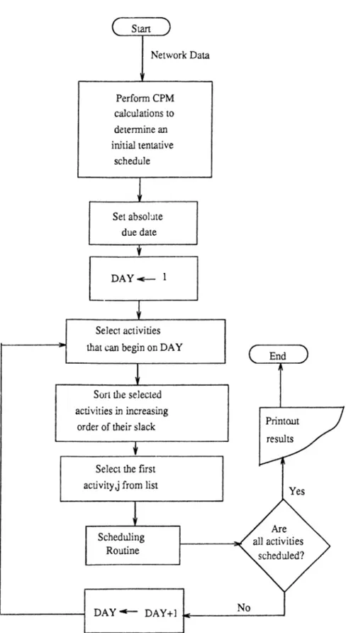
The steps involved in MINSLK heuristic are shown in a flow chart form in Figure 3.1-3.2. The MINSLK is based essentially on three rules:

i) Resources are allocated serially in time. That is, it starts on the first day and schedule aU

activities possible, then advance to the next day and do the same.

it) In case more than one activity compete for the same resources, rank them in the order of

minimum activity slack.

in) Reschedule noncritical activities, if possible, so as to free resources for scheduling critical

activities-those activities which has no slack.

A brief description of different steps is as follows:

Step 1

All initial tentative schedule is determined without taking any resource constraints into ac­ count via CPM calculations. This schedule only reflects restrictions placed on the start ond finish times. It is tried to schedule each activity at its early start time. Start the first day of the

CHAPTER 3. PROBLEM FORMULATION AND SOLUTION PROCEDURES 16

project. Set DAY to 1.

Step 2

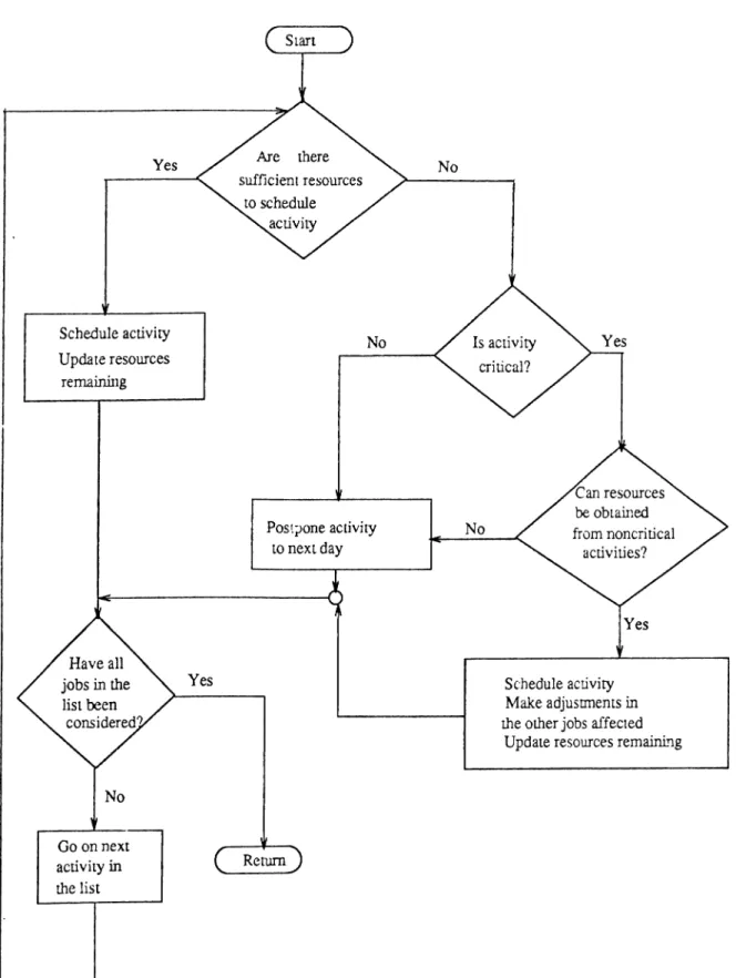
All the activities that are eligible to start on DAY are arranged in a waiting list sorted in increasing order of activity slack. For each activity the MINSLK checks to see whether there are sufficient resources avaliable or not. If enough resources are available, the ongoing activity is scheduled to start on DAY. Otherwise, it is checked whether the activity is critical(ie, it has no slack) or not, non-critical activities being postponed to the next day. In case the activity is critical, rescheduling of activities is done to obtain resources from already scheduled non-critical activities. If rescheduling is not possible the activity will be postponed to the next day.

Step 3

If all activities in the waiting list are considered, DAY is advanced to the next day and aU the steps are repeated again until there are no more activities to schedule.

S D F IR S T H eu ristic

The mode of operation of SDFIRST is the same as MINSLK except the followings :

i) The activity that has a less duration time is tried to schedule first if there are more than

one activity awaiting to be scheduled.

it) The rescheduling routine is not included. That is. the criticcJ activity which requires more

resources than available wiU be posponed to the next day.

L D F IR S T H eu ristic

The LDFIRST heuristic has the same operational characteristics with SDFIRST except the fact that it gets the activity that has longer duration time as first among the competing activities.

CHAPTER 3. P R O B L E M F O R M U L A T IO N A N D S O L U T IO N P R O C E D U R E S 17

3 .2 .3 O p t im iz in g S o ftw a re S C I C O N I C

An optimum seeking solution software, SCICONIC/VM V I.47 is used on tlie mainframe Data General MV/2000. It is a professional package which is mainly designed to solve linear and non-linear programming problems. A branch and bound subroutine is embedded in it to find out solutions for integer programming problems.

In order to have integer solutions by SCICONIC in a reasonable amount of time , it is de­ cided to reduce the 0-1 formulation of the problem in size. The reduction process is based on the fact that the problem size is dependent on activity duration times, dj. In reduction process,

the time unit is scaled down by a predetermined factor. It is achieved through dividing activity durations by a predetermined scale factor keeping other input parameters same in the genera­ tion process of the test problem. Then, the scaled problem has smaller number of variables and constraints. In order to keep the integrality of data, the divisions are truncated to the nearest integer. After handling of a feasible integer solution by SCICONIC, the value of the objective function is updated by multiplying scale factor in rescaling process. However, it should be kept in mind that this results in a information loss in the value of the objective function as well as the possibility of having no feasible integer solution at aU due to scaling and rescaling of the problem.

CHAPTER 3. PROBLEM FORMULATION AND SOLUTION PROCEDURES 18

CHAPTER 3. PROBLEM FORMULATION AND SOLUTION PROCEDURES 19

Chapter 4

EXPERIMENTATION AND

RESULTS

In this chapter, details of the generation of test problems are given. In Section 4.2, the design of analysis is discussed. We provide the results of the study in Section 4.3.

4.1

Problem Generation

In order to test the performance of solution procedures, a problem generator called NGNR, is coded in Pascal. A standard random number generator is embedded in the procedure seeking the objectives o f :

i.) generating different problems,

ii.) making it easier to regenerate the same problem with the same set of input parameters.

NGNR performs the following steps to generate a problem :

Step 1 : Read the following input parameters that are grouped into two :

i.) Set of parameters related to problem characteristics :

+ Number of nodes, called nnode, in the project w’here a node repre.sents the start

or end of a activity,

+ Upper limit on the number of preceding activities in the project,

CHAPTER 4. EXPERIMENTATION AND RESULTS 21

+ Upper limit on the number of succeding activities in the project, * Number of different resource types,

* Lower and upper limits on the resource consumption rates , * Range for the duration o f activities,

* Resource tightness ratio, called rt, that is used to calculate the resource avalia- bilities,

* Critical path duration multiplier, called dm that is used to set the absolute due

date ,T

* Scale parameter, called scale, that is needed to reduce the problem in size for the

solution procedure, SCICONIC.

ii.) Set of parameters used by NGNR :

+ Initial seed for the random number generator,

* Upper bound on the number of iterations that is needed to produce incidence matrix, called niter.

Step 2 : Generate the incidence matrix in niter number of iterations. The incidence

matrix, called NETWORK is a nnodexnnode upper triangle matrix that is used to define

the precedence relationships in the project network. For example, if there is an activity whose starting event is i and ending event j , then NETWORK[i,y] is set to 1. Activities

are represented by arcs whereas events by nodes in the project network. All arcs are unidirected w'hose head shows its starting node and tail represents its ending node. The project has only one starting and ending node.

Step 3 : Update the incidence matrix in order to have a complete project network, ie,

append new arcs emanating from unconnected nodes to the ending node.

Step 4 : Determine the followings for each generated arc :

- Its starting node, - Its ending node,

- Activity duration time, dj. Note that reduction process discussed in Section 3.2.3. is

achieved through dividing the duration time by scale parameter, scale, - Each resource requirement, rjk,

- The predecessor set that is all the activities that precede the ongoing activity, - The successor set which is aU the activities that succédé the ongoing activity.

Step 5 : Perform CPM calculations which results in computed values of :

- Early start and finish time, - Latest start and finish time.

CHAPTER 4. EXPERIMENTATION AND RESULTS ₂₂

— Total and free slack-used only by MINSLK, SDFISRT and LDFISRT Heuristics, — Critical path duration,

— Absolute due date, T that is set to critical path duration times dm.

Step 6 : Determine the peak resource requirements.

Step 7 : Compute the resource availability for each resource type, Rkt through multiplying

peak resource requirement by resource tightness ratio, rt.

Step 8 : Make necessary arrangements in order to output the problem in the form of

formulation that was discussed in Section 3.1.

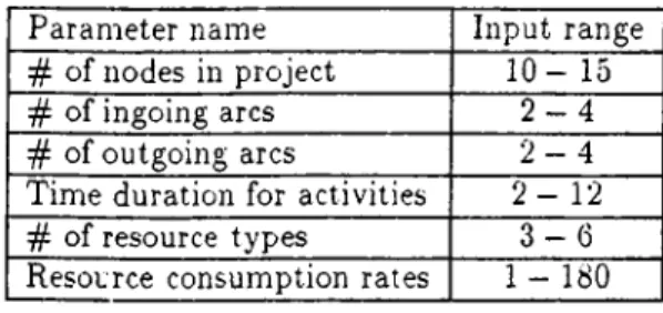
The input range for parameters is tabulated in Table 4.1.

P aram eter name Input range # o f nodes in p ro je ct 1 0 - 15 # o f ingoing arcs 2 - 4 # o f ou tg oin g arcs 2 - 4 T im e duration for activities 2 - 1 2 # o f resource types 3 — 6 R esource con su m ption rates 1 - 180

Table 4.1: The input range for parameters

4.2

Design of Analysis

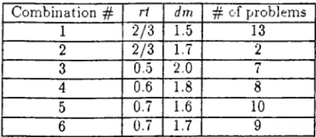
As discussed in Section 4.1, there are two parameters involved in generation process which are resource tightness ratio and critical path duration multiplier. The experiment is carried out with different combinations of them. In each combination, each problem is generated using a different initial seed to incorporate the randomness. A list of combinations together with number of test problems in each one is given in Table 4.2.

The feasibility o f the problem is sensitive to these two factors.As the resource tightness ra­ tio increases, the problem becomes more difficult. The idea behind the critical path duration multiplier is to allow the project finished later than its respective critical path duration. As it increases, the feasibibty of the problem becomes more bkely.

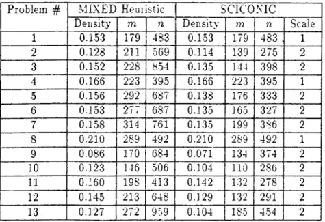
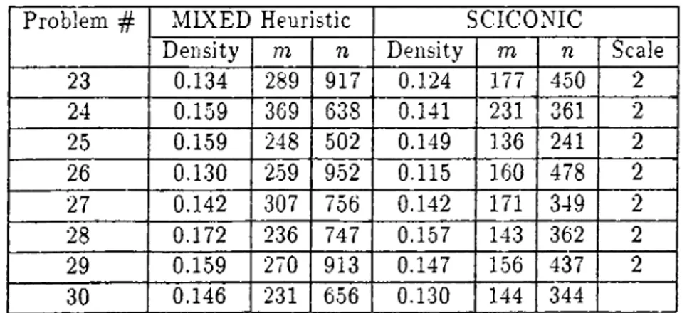
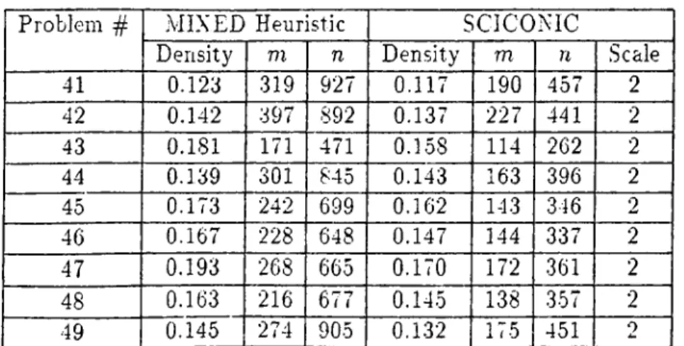
The generated problems together with their sizes and densities in their respective group are given in Tables A1.-A6. in Appendix . Since the problem is reduced by a scale factor for the input to SCICONIC, the scale factors are given in its corresponding column. In those tables, m

CHAPTER 4. EXPERIMENTATION AND RESULTS 23

denotes the number of constraints and n shows the number of variables.

The test problems have activities ranging from 16 to 36. The number o f constraints in the formulated problems changes between 114 and 397 and the number of variables is in between 241 and 969.The density of the problems range from 0.071 to 0.210.

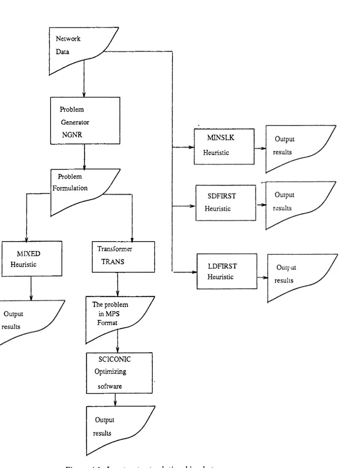
It is noted that a transformation process is necessary before SCICONIC starts to run. So, a program, called TRANS is coded in pascal to arrange the output of problem generator, NGNR in the form of MPS-Mathematical Programming System format. For a clear understanding, the

input-output relationships between the programs is given in Figure 4.1.

C om b in a tion # ri dm # o f p rob lem s 1 2 /3 1.5 13 2 2 /3 1.7 2 3 0.5 2.0 rr/ 4 0.6 1.8 8 5 0.7 1.6 10 6 0.7 1.7 9

CHAPTER 4. EXPERIMENTATION AND RESULTS ₂₄

4.3 Results of the Study

As it. is stated in Section 3.2.1, MIXED heuristic works with a penalty function. So, it in­ volves a choice of penalties associated with job completion, precedence relationships, resource, nonnegativity and upper bound constraints in order to get a feasible solution for the problem. In detail, the following strategy in setting penalty weights and executing MINSLK heuristic is implemented :

The penalties, Vj and Wj corresponding to nonnegativity and upper bound constraints are

set at least twice greater than the penalties assigned to job completion constraints,PCl. They are kept equal in aU test problems (vj = wj, Vj). The penalties for precedence relatonships

and resource constraints, PC2 and PCS respectively, are always less than the penalty weight

associated with job completion constraints. PCS is experimentally selected by taking the com­

bination of resource tightness ratio and critical path duration multiplier into account. It is at most equal to PC2. If the execution of MINSLK heuristic results in violated constraints with

the ongoing set of penalties, the penalty weights corresponding to violated ones are updated and the heuristic is executed again.

On the other hand, due to the fact that the optimizing software, SCICONIC uses branch and bound technique to solve integer programming problems, some stopping criteria are introduced to stop further branching. An integer solution that has a objective value within 90% proximity of its corresponding linear optimum solution excluding the objective constant, uj, discussed

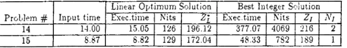
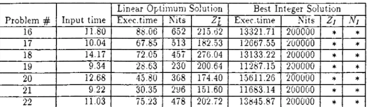
in Section 3.1 is taken to be sufficient. Moreover, maximum CPU time, in seconds allowed is constrained to 18,000 seconds and maximum number of iterations is to 200,000. The compu­ tational results are given in Tables A .7 - A .12 in Appendix. In those tables, the followings are provided :

• Input time in CPU seconds, • Linear optimum solution

- optimum objective value, Z£ - execution time in CPU seconds - ^ of iterations. Nits

• Best Integer solution - objective vadue, Zj

- execution time in CPU seconds, excluding the time required to find linear optimum

CHAPTER 4. EXPERIMENTATION AND RESULTS ₂₅

— # of iterations, Nits

- ^ oi integer solutions found by the time it terminates. Ni

It is noted that S ’ means the execution is interrupted due to either CPU time hmit or iter­ ations limit without yielding a feasible integer solution.

The execution results of heuristics are tabulated in Tables A .13 - A .18 in Appendix.In the column of MIXED heuristics, the input and executed CPU seconds are provided separately. It is also given the number of repetitions performed to end up with a feasible solution. It is kept in mind that S + ’ shows that the heuristic does not achieve a feasible integer solution. On the other hand, we will not supply the CPU times of those heuristics, MINSLK, SDFIRST and LDFIRST due to the fact that they solve aU problems in a few seconds. The linear optimum and best integer solution found so far by SCICONIC is appended to those tables. It is noted that the objective function values are corrected by the scale parameter, scale.

Out o f 49 problems, the optimizing software, SCICONIC is unable to find a feasible integer solution for 13 problems in the allowable time span and number of iterations. For those of prob­ lems ,in combination ^^3, that are tightly resource constrained, it does not provide any feasible integer solution. It is interrupted in 27 problems in order not to let further branching. On the other hand, a feasible integer solution for 14 problems is not achieved by the heuristics, MIXED whereas the remaining heuristics come up with a feasible solution for all test problems. The num­ ber of problems that both SCICONIC and MIXED heuristic can not yield a feasible solution is 8.

Table A .19 in Appendix shows the solution procedure that achieves the best solution for the respective problem on the basis of objective function value.

Considering aU test problems, the number of times SCICONIC yields the best solution is 21, MINSLK heuristic is 18, SDFIRST is 10, LDFIRST is 2 and MIXED is none.

On the average, the solutions given by SCICONIC are within 9.23% of their respective linear optimum values covering only those problems that it is ended with feasible integer solutions. On the other hand, MIXED heuristic provides integer solutions that are deviated 31.59% from their corresponding linear optimum solution for those problems in which the heuristic finds a feasible integer solution. For the other heuristics, the average(in %) deviation from linear optimum

CHAPTER 4. EXPERIMENTATION AND RESULTS 26

. MINSLK ...15.91% . S D F IR S T ...14.03% . L D F IR S T ...19.74%

For those of problems equipped with feasible integer solutions by MIXED heuristics, average time to spent is found to be 1778 CPU secondss including the number of repetitions. On the other hand, in spite of stopping execution conditions, SCICONIC spents 6055 CPU seconds on the average. It takes an average of 27 seconds to find out linear optimum solutions.

CHAPTER 4, EXPERlMENTATlOy AND RESULTS Network Data Problem Generator NGNR Problem Formulation M IXED Heuristic Transformer TRANS The problem inMPS Format MINSLK Heuristic 11 SCICONIC Optimizing software Output results

Chapter 5

CONCLUSIONS AND

RECOMMENDATIONS

Based on the results obtained from the experiment, we can state the following ;

(1) From computational effort point of view, the heuristics MINSLK, SDFIRST and LDFIRST are found to be better. This is expected since these heuristics are specially suited for project scheduling problems and they are single-pass type algorithms.

(2) On the basis of both number of times yielding the best solution and deviation from linear optimum, the heuristic LDFIRST is worse than the other two. Although MINSLK heuristic is better than SDFIRST in view of the number cases achieved the best solution, SDFIRST has a better solution quality.

(3) The percent deviation from linear optimum through these single-pass typed heuristics is sensitive to the problem difficulty.

(4) SCICONIC is the best performing in the set of problems that is included in combination ^ 4 and SDFIRST heuristic is in combination ^3. But, there is no dominating solution

procedure if aU the cases are taken into account.

(5) The solution quality by SCICONTC is better than the others.

In view of the experiment, the heuristic, MIXED looks to be inappropriate for such type of problems. But, there may be scope by a judicious selection mechanism of penalty weights and starting solution.

CHAPTER 5. CONCLUSIONS AND RECOMMENDATIONS 29

Although the solution quality obtained by SCICONIC is found to be better than others, its time and memory requirements are prohibitive for even mediumi-sized problems.

It may be worthy to solve the problem with the tested heuristics and select the best among them.

As a further research issue, a st udy including other performance criteria together with other sequencing rules in single or multiple project environments may be conducted. It may also include the decomposition approach.

Appendix A

APPENDIX A. 31

Problem ^5^ MIXED Heuristic SCICONIC

Density m n Density m n Scale

1 0.153 179 483 0.153 179 483 . 1 2 0,128 211 569 0.114 139 275 2 3 0.1-52 228 8-54 0.135 144 398 2 4 0.166 223 395 0.166 223 395 1 5 0.156 292 687 0.138 176 3.33 2 6 0.153 277 687 0.135 165 327 2 7 0.158 314 761 0.135 199 386 2 8 0.210 289 492 0.210 289 492 1 9 0.086 170 684 0.071 134 374 2 10 0.123 146 506 0.104

no

Table A .l: The size and density of the generated problems in combination

Problem ^ MIXED Heuristic SCICONIC

Density m n Density 777 n Scale

14 0.156 344 834 0.144 204 421 2

15 0.152 235 796 0.135 145 372 2

APPENDIX A. ₃₂

Problem # MIXED Heuristic SCICONIC

Density m n Density m n Scale

16 0.136 257 961 0.125 161 511 2 17 0.111 259 969 0.102 163 475 2 18 0.145 341 840 0.129 216 451 2 19 0.141 283 680 0.118 179 369 2 20 0.140 289 934 0.139 163 434 2 21 0.123 235 900 0.114 145 448 2 22 r 0.129 319 866 0.121 187 417 2

Table A.3: The size and density of the generated problems in combination ^ 3

Problem # MIXED Heuristic SCICONIC

Density m n Density m n Scale

23 0.134 289 917 0.124 177 450 2 24 0.159 369 638 0.141 231 361 2 25 0.159 248 502 0.149 136 241 2 26 0.1.30 259 952 0.115 160 478 2 27 0.142 307 756 0.142 171 349 2 28 0.172 236 747 0.157 143 362 2 29 0.159 270 913 0.147 156 437 2 30 0.146 231 656 0.130 144 344

AFPENDIX A. ₃₃

Problem MIXED Heuristic SCICONIC

Density m n Density in n Scale

3] 0.141 . 176 695 0.122 114 .340 2 32 0.169 213 730 0.143 141 386 2 33 0.164 318 928 0.147 190 456 2 34 0.155 344 761 0.141 196 372 2 35 0.126 344 822 0.121 181 394 2 3Ö 0.175 215 576 0.150 137 304 2 37 0.148 318 723 0.135 186 372 2 38 0.195 377 787 0.178 217 389 2 39 0.178 230 629 0.158 143 312 2 40 0.167 265 792 0.151 166 424 2

Table A .5: The size and density of the generated problems in combination

Problem # .MIXED Heuristic SCICONIC

Density 771 n _Density 771 n Scale

41 0.123 319 927 0.117 190 457 2 42 0.142 397 892 0.137 227 441 2 43 0.181 171 471 0.158 114 262 2 44 0.139 301 845 0.143 163 396 2 45 0.173 242 699 0.162 143 346 2 46 0.167 228 648 0.147 144 337 2 47 0.193 268 665 0.170 172 361 2 48 0.163 216 677 0.145 138 357 2 49 0.145 274 905 0.132 175 451 2

APPENDIX A. ₃₄

P rob lem 7,^ Input tim e

Linear O p tim u m Solution Best Integer Solution E xec.tim e Nits _{^ 2} Exec, tim e Nits N j

1 14.89 53.24 395 311.87 12681.93 200000 348 5 2 5.43 20.06 279 151.74 13709.34 200000 174 6 3 9.07 21.30 284 217.40 97.15 1415 234 1 4 16.32 81.56 457 333.28 18000.00 ♦ _* * 5 9.50 42,89 378 222.79 13457.66 200000 245 8 6 8.95 17.30 203 193.42 55.35 784 203 1 7 11.77 10.78 134 164.40 61.57 790 165 1 8 24.92 78.84 383 328.00 18000.00 * * ♦ 9 5.12 6.95 143 164.87 26.46 360 171 1 10 4.11 9.32 193 139.75 61.63 1297 151 2 11 6.25 37.62 360 229.77 10018.98 200000 278 8 12 6 .2 1 20.32 285 188.36 10671.60 200000 220 1 13 10.32 12.42 167 352.03 172.46 1969 1 358 3

Table A .7: The results by SCICONIC for the test problems in combination

P rob lem # Input tim e

Linear O p tim u m S olution Best Integer Solution Exec, tim e Nits _{Z i} Exec, tim e Nits _N1 14 14,00 15.05 126 196.12 377.07 4069 216 2 15 8.87 8.82 129 172.04 48.33 782 189 1

APPENDIX A. 35

P rob lem # Input tim e

Linear O p tim u m Solution Best Integer S olu tion E xec.tim e Nits _Zl E xec, tim e Nits 2 ; N j

16 11.80 88.06 652 215.0*2 13321.71 200000 * * 17 10.04 67.85 513 182..53 12667.55 200000 * * 18 14.17 72.05 457 276.04 13133.22 200000 * * 19 9.34 28.63 230 200.64 11287.15 200000 * * 20 12.68 45.80 368 174.40 1.5611.26 200000 * * 21 9.22 30.35 296 151.60 11683.14 200000 * * 22 11.03 75.23 478 202.72 13845.87 200000 * *

Table A .9: The results by SCICONTC for the test problems in combination # 3

P roblem # Input tim e

Linear O p tim u m Solution Best Integer S olu tion Fxvic.tiine Nits E xec, tim e Nits Z r N j

23 11.59 37.67 329 193.37 11680.78 160740 215 4 24 13.00 58.14 400 182.84 14122.04 200000 * * 25 5.95 8.59 133 92.09 12679.98 200000 103 2 26 10.98 33.75 316 217.51 144.92 1680 •237 2 27 9.91 39.79 361 147.17 13668.70 200000 169 11 28 9.-54 29.09 295 181.67 14608.80 200000 201 7 29 11.61 21.90 208 231.00 14117.44 200000 257 3 30 7.83 16.41 200 155.87 2083.13 33445 172 6

APPENDIX A. 36

P rob lem # Input tim e

Linear O p tim u m Solui.ion Best Integer Solution Exec, tim e Nits E xec.tim e Nits ^7 N i

31 6.24 5.38 101 139.47 12617.98 200000 146 1 32 9.17 23.73 ^ 298 206.35 56.08 696 223 1 33 14.19 33.23 274 213.14 16525.30 200000 237 7 34 11.44 22.68 267 198.68 15823.45 200000 244 1 35 9.82 21.50 219 306.81 13872.20 200000 * * 36 7.59 11.31 162 181.80 15143.05 200000 192 1 37 10.41 23.59 259 191.34 717.94 9918 209 4 38 16.27 42.04 306 244.06 171.74 1644 250 2 39 8.45 9.63 148 208.80 33.51 523 221 1 40 12.31 38.74 338 2.52.18 177.12 2071 268 1

Table A. 11: The results by SCICONIC for the test problems in combination

P ro b le m # Input tim e

Linear O p tim u m Solution Best Integer Solution E xec.tim e Nits E xec, tim e Nits Ni

41 11.64 88.03 739 320.54 15124.75 200000 * 42 15.27 23.54 224 211.81 106.98 1145 233 1 43 5.77 18.60 275 130.78 9854.61 200O00 146 6 44 10.69 7.33 88 158.29 242.84 2634 177 1 45 9.41 32.11 345 221.08 12125.34 200000 + * 46 8.47 19.94 230 162.05 309.44 4551 178 4 47 11.82 25.00 267 184.14 63.21 759 195 1 48 8.45 8.43 126 189.41 20.39 317 193 2 49 12.01 62.36 524 296.57 14824.61 179269 318 4

APPENDIX A. ₃₇

M IX E D M IN SLK S D F IR S T L D F iR S T S C IC O N IC # o f T iiiie(secs) ^ b j . O b j. O b j. O b j. Linear Integer P rob lem trials Input Exec. value value value value Z i

1 2 20.15 875.67 473 350 353 382 311.87 348 2 2 27.70 583.38 386 362 358 31:^5 303.48 348 3 1 45.90 3379.89 563 4-56 475 457 4.34.80 468 4 2 Jtcjjc 409 382 3a4 333.28 * 5 1 50.65 2667.09 627 536 520 584 445.56 490 6 1 43.99 774.64 571 419 458 4*j5 386.84 406 7 1 58.05 1078.12 382 338 344 3vJ 328.80 330 8 1 33.50 1065.30 486 347 369 0 - 0 328.00 * 9 1 27.68 5.52.58 343 332 334 r, .• j ·.'· J 329.74 ;342 10 1 17.06 248.13 308 319 312 315 279.50 302 11 2 ** ** 518 542 544 459.54 556 12 1 32.09 652.02 430 380 393 3^8 376.72 440 13 3 ** * 7-58 778 7o2 7a4.06 716

Table A .13: The computational re;.alts by heuristics for the test problems in combination #1

P ro b le m # M IX E D M IN SLK SDF1R.ST L D F IR S T SCICO.NIC # o f trials T im e(secs) O b j. value O b j. value O b j. value O t j. value Linear Integer Z i Input Exec. 14 1 65.15 958.09 481 425 437 426 392.24 432 15 1 42.47 1056.01 428 389 405 377 344.08 378

APPENDIX A. ₃₈ P rob lem # M IX E D MLXSLK S D F IR S T L D f I R S T .SCICONIC # o f trials T im e (secs) O b j. value O b j. value O b j. value O b j. ^·alue Linear Integer Z j Input Exec. 16 1 56.55 33'29.54 611 588 543 587 431.24 * 17 4 ** ** 452 436 463 365.06 * 18 2 ** ** 701 728 756 552.08 * 19 5 ** 503 471 512 401.28 * 20 1 61.65 3985.65 522 440 ■ 396 462 348.80 * 21 3 47.36 3914.14 439 401 337 426 303.20 * 22 2 ** 523 524 580 405.44 ¥

Table A. 15: The computational results by heuristics for the test problems in combination #3

P rob lem # M IX E D M IX S L K .SDFIR.ST L D F IR S T S C IC O N IC # o f trials T im e(secs) O b j. voJue O b j. value O b j. value O b j. value Linear Integer Input Exec. 23 1 59.34 5331.42 .569 511 481 462 386.74 430 24 2 ** 527 493 501 365.68 * 25 1 28.71 645.72 324 259 210 297 184.18 206 26 2 ** ** 512 494 537 435.02 474 27 1 57.78 1360.78 440 398 320 378 294.34 338 28 1 ^ 1 . 6 8 719.40 497 413 435 444 363.34 402 29 1 ^ 8 . 4 0 4214.27- 593 537 560 549 462.00 514 30 1 56.52 900.84 479 356 354 1 380 311.74 344

APPE.XDIX A. ₃₉

P rob lem #

-MIXED -MINSl.K S D E IR S T L D F IR S T .SCIGONIC # o f trials T i m e ( s e c s ) O b j. value O b j. value O b j. value O b j. value Linear Integer Input E x e c . 31 1 30,35 378.30 326 307 302 315 278.94 292 32 1 38.45 1270.00 521 447 4 / 8 480 412.70 446 33 1 74.53 303-l.o3 5.59 499 530 509 426.28 474 34 3 + + 487 494 520 397.36 488 35 2 680 697 721 613.62 * 36 2 2 8 .G2 1033.58 497 415 394 415 363.60 384 37 2 467 419 455 382.68 418 38 2 ** * * 502 515 534 488.12 500 39 2 34,55 1231.55 502 4*J() 428 435 417.60 442 40 1 4S.AJ 2301,11 576 5 i 7 543 oGO 504.36 536

Table A .17: The comp .rational results by heuristics for the test problems in combination

P ro b le m # M IX E D M IX S L K S D E IR S T L D F IR S T S C IC O N IC # o f trials Tirjie(sccs) O b j. value O b j. value O b j. value O b j. value Liiibiar Integer Input Exec. 41 2 + * ** 680 697 721 641,08 * 42 1 82.73 3105.31 510 475 454 485 423.62 " 466 43 1 18.48 371.63 389 329 297 307 261.56 292 44 1 58.44 742.44 380 344 370 396 316.58 .3.54 45 1 38..58 2366..56 678 530 523 573 442.16 46 1 35.52 655.71 454 356 358 375 32.1.10 356 47 1 42.76 1208,26 430 396 372 397 36^.2S 390 48 1 34.60 621.78 384 382 392 382 3 < 8.8 2 3S6 49 1 56..52 18sO,6C 724 645 635 680 593.14 636

AP.PENDIX A. ₄₀

Problem # MIXED MINSLK SDFIRST LDFIRST SCICONIC

1 * 2 3 4 * 5 * 6 * 7 * 8 * 9 * 10 * 11 * 12 i 13 * 14 * 15 * 16 * 17 * 18 19 * 20 * 21 * 22 * 23 * 24 * 25 *

APPEJ^DIX .4. 41

Problem # MIXED MIXSLK SDFIRST LDFIRST SCirO N lC

26 * 27 * * 28 * 29 * 30 * 31 * 32 * 33 * 34 * 35 * 36 * 37 * 38 * 39 * 40 * 41 * 42 * 43 44 * 45 * 46 * * 47 * 48 * * 49 * Total - 18 10 2 21 Table A. 19: continued

Bibliography

[1] Bell C.E. and Han J., ” A New Heuristic Solution Method in Resource-Constrained Project Scheduling” , Naval Research Logistics, 38 (1991), 315-331.

[2] Boctor F.F, ’’ Some Efficient Multi-Heuristic Procedures for Resource Constrained Project Scheduling” , Europ.J.Op.Res 49 (1990), 3-13.

[3] Christofides N., Valdes R.A. and Tamarit J.M., ’’ Project Scheduling With Resource Con­ straints : A Branch and Bound Approach” , Europ.J.Oper.Res. 29 (1987), 262-273.

[4] Cooper D.F., ” Heuristics for Scheduling Resource Constrained Projects : An E.xperimental Investigation” , Man.Sci. 22, 11 (July 1976), 1186-1184.

[5] Davis E.W .,’’ Networks ;resource allocation” , J.Ind.Eng. (1974).

[6] Davis E.W. and Heidorn G.E., ” An Algorithm for Optimal Scheduling Under Multiple Resource Constraints” , Man.Sci. 17, 12 (1971), B803-B816.

[7] Davis E.W. and Patterson J.H., ” A Comparison of Heuristic and Optimum Solutions in Resource-Constrained Project Scheduling” , Man.Sci. 21, 8 (1975), 944-955.

[8] Deckro R.F., Winkofsky E.P., Hebert J.E. and Gagnon R., ” A Decomposition Approach to Multi-project Scheduhng” , Europ.J.Oper.Res. 51 (1991), 110-118.

[9] Elsa}’ed E.A. and Nasr N.Z., ’‘ Heuristics for Resource Constrained Scheduling” ,

Int.J.Oper.Res. 24, 2 (1986), 299-310.

[10] Fendly L.G., ’’ Toward the Development of a Complete Multiproject Scheduling System” ,

J.Ind.Eng. 19, 10 (1968), 505-515.

[11] Fisher M.L., ’’ Optimum Solution of Problems Using Lagrange Multipliers;Part I” , Ope r.Res.

(1973), 1115-11-27.

[12] Holloway C.A.,Nelson R.T. and Suraphongschai V., ’’ Comparison of a Multi-Pass Heuris­ tic Decomposition Procedure with other Resource-Constrained Project Scheduling Proce­ dures” , Man.Sci. 25, 9 (1979), 862-872.